* Economic and Commercial Office of the Embassy of Spain, Belgrade
** Faculty of Economics, University of Belgrade, urosevic@ekof.bg.ac.rs. Branko Urošević gratefully acknowledges support by the Serbian Ministry of Science and Technology, Grant No 149041.
JEL CLASSIFICATION: C02, C60, G10, G12, G21 ABSTRACT: Pure econometric approaches
to pricing mortgage-backed securities (MBSs) - principal pricing vehicles used by financial practitioners - fail to capture their true risks. This point was powerfully driven home by the global financial crisis. Since prior to the crisis default rates of MBSs were quite modest, econometric pricing models systematically underestimated the possibility of default. As a result, MBSs were severely overvalued. It is widely believed that the global crisis was largely triggered by incorrect valuation of mortgage-backed securities. In the aftermath, it is important to revisit the foundations for pricing
MBSs and to pay much closer attention to default risk. This paper introduces a comprehensive model for valuation of fixed-rate pass-through mortgage-backed securities in a simple option-based framework. In the model, we use bivariate binomial tree approach to simultaneously model prepayment and default options. Our simulation results demonstrate that the proposed model has sufficient flexibility to capture the two principal risks.
KEY WORDS: mortgage-backed security (MBS), prepayment, default, bivariate binomial pricing technique
DOI:10.2298/EKA1086042M
Ana Manola* and Branko Urošević**
OPTION-BASED VALUATION OF
MORTGAGE-BACKED SECURITIES
1. INTRODUCTION
Mispricing of mortgage-backed securities (MBS) has been widely blamed for triggering the recent global financial crisis. In a nutshell, these securities are portfolios consisting of a large number of individual residential mortgage loans. It is well known that individual mortgage loans can be prematurely terminated because a borrower has either prepaid or defaulted on the loan. Rather shockingly, the models used by rating agencies, in particular, seemed to largely understate the possibility of borrower default. The aim of this paper is to present an option-based framework for pricing MBSs. It incorporates both defaults and prepayments of individual mortgages. It compares two different approaches for modelling mortgage termination and studies the importance of default in the model.
Historically there have been two different approaches to modelling MBSs – econometric and option-based models.
Econometric models focus on MBS asset as a whole. They specify a particular functional relationship that captures mortgage termination patterns. They are, then, calibrated on historical termination data and used to project cash flows over the life of the security. Different explanatory variables can be used, such as: ratio of coupon and long-term interest rate (to capture an incentive to refinance), pool factor (to capture burnout effect), a seasonal dummy variable (to capture seasoning effect), macroeconomic variables such as level, slope, and recent history of interest rates, change in housing prices, unemployment rate, GDP growth, or different pool characteristics that capture borrowers’ personal characteristics1. These models typically apply a forward-looking pricing technique based on Monte Carlo simulation.
Option-based models start with individual mortgages. These models treat the mortgage as a bond with two embedded options: an American call option (the option to prepay) and a series of European put options (the option to default). There are several models of pricing individual mortgage loans. These models vary in the manner in which they address the borrower’s decision to terminate the mortgage and in the manner in which they treat the heterogeneity of borrowers. As a borrower’s termination decision is based on his/her anticipation of the future, 1 Some types of functional forms and different choices of explanatory variables can be found
a backward technique is typically employed for solving the valuation problem of an individual mortgage loan.
The recent financial crisis pointed out the weak spots in the financial system as a whole. Among them, it became obvious that the models used by financial institutions failed to adequately price risks related to MBSs. Careful modelling of default rose to prominence.
Historically financial institutions primarily used econometric models. These models did not put much emphasis on default as mortgage pools were mostly seen as of low default risk due to agencies’ guarantees, while securitization was perceived to mitigate default risk. Thus the issue of default was either completely ignored or treated exogenously by projecting a certain default rate2. This was partly due to insufficient data on individual contracts underlying the security, aggregated information, and short history of available data. Schwartz and Torous (1992) stress the importance of joint consideration of prepayment and default, acknowledging that defaults can significantly change patterns of MBS cash flows. Until the crisis hit, option-based MBS pricing models were mostly ignored by practitioners. Apart from being more complicated to implement than their econometric counterparts, they were criticized for imposing an upper bound to the values of MBSs that is not observed in practice3.
Early option-based models addressed the borrower’s decision assuming interest rate as the only source of risk. For example, Dunn and McConnell (1981) modelled MBS as an annuity with embedded American call option, ignoring default and assuming no transaction costs related to prepayments4. These models focused more on the economic environment and backward algorithm applied than on careful modelling of a borrower’s decision.
2 As late as 2001, historical evidence pointed to low rates of default (less than 0.5% of conditional prepayment rate on average). Based on this historical data, many investment banks modelled default using the Standard Default Assumption Curve developed by the Bond Market Association. See Salomon Smith Barney (2001).
3 The MBS prices obtained were capped by par plus transaction costs, see Stanton (1995) and Longstaff (2002).
4 Discussion of the early models in literature can be found in Hendershott and VanOrder (1987). See also Kau et al. (1992), Kau and Keenan (1995), and Kalotay, Yang and Fabozzi (2004).
Different authors note that borrowers often do not prepay optimally. In order to capture that fact they introduce transaction costs and other sorts of frictions5. However, all these early models assume homogeneity of classes of borrowers, so that refinancing occurs simultaneously in the entire pool. Thus, when interest rates reach the critical level again, there will be no further borrowers to prepay. These models lack power to explain seasonality and to capture the possibility that some borrowers prepay when it is financially not optimal to do so, or forego prepaying when it is financially optimal.
In order to overcome this problem, Stanton (1995) introduces heterogeneity of borrowers. He assumes that mortgagors face heterogeneous transaction costs measured as fractions of the unpaid mortgage balance and governed by beta distribution. Further, he assumes a probability of exogenous prepayment modelled by a hazard function. The assumption that a prepayment decision can be made only at random discrete time intervals prevents the situation from occurring in which all borrowers of a certain transaction cost level prepay immediately once the interest rate reaches a critical level. While this was a significant modelling breakthrough, there was one major drawback. Namely, the interest rate is assumed to be the sole source of risk. Stanton’s work is later extended by Downing, Stanton and Wallace (2003) to include the possibility of default.
From the beginning of the option-based approach to mortgage valuation, default was recognized as part of a borrower’s decision6. Various authors recognize the default option as an inseparable part of valuation, which as such should be simultaneously modelled with prepayment7. The source of uncertainty that influences a borrower’s decision to default is the value of the collateral, i.e. the level of house prices. Kau and Slawson (2002) introduce frictions in this framework to account for heterogeneity of borrowers and for exogenous terminations resulting from the borrower’s characteristics8.
Prepayment and default options compete with each other in that by exercising one the other is rendered worthless. Namely, if a borrower defaults s/he cannot prepay and vice-versa. The borrower, in a rational framework, chooses the timing 5 Early models already recognized that borrowers often do not act in a rational manner. For example, Dunn and McConnel (1981) allowed for sub-optimal prepayments triggered by realizations of a Poisson process. For more references, see Kalotay, Yang and Fabozzi (2004). 6 See Bardhan et al (2006), Kau et al. (1992) and Kau and Keenan (1995).
7 See Kau et al. (1992), Kau and Keenan (1995), Deng, Quigley and Van Order (1995).
and type of mortgage termination that minimizes his/her liability. Thus, these two options must be valued simultaneously.
More recently, Kalotay, Young and Fabozzi (2004) introduce the idea of using two different yield curves when pricing MBS – one for modelling the refinancing strategy of borrowers, the other for discounting MBS cash flows. Longstaff (2002) incorporated the credit spread of the borrower into his refinancing decision. He also applied Longstaff and Schwartz least-squares method to solve for optimal strategy. A group of authors (Goncharov (2005), Kolbe and Zagst (2007)) emphasize the intensity-based approach to value mortgage contract and MBS. In this paper we focus on fixed-rate residential pass-through MBSs as the most common segment of the market. We present two models to value such securities. In particular, we combine heterogeneity of borrowers as modelled in Downing, Stanton and Wallace (2003) with a specific option-based model for pricing individual mortgages. One is the model presented in Downing, Stanton and Wallace (2003) while the other is the mortgage valuation technique of Kau and Slawson (2002). Our paper is, to the best of our knowledge, the first paper to do so. We compare and contrast the two methods of pricing pass-through securities focusing, in particular, on the role of borrowers’ defaults. Both of these models are flexible and can capture many realistic features of borrower behaviour. 2. VALUATION PROCEDURE
The modelling takes a bottom-up approach and views MBS as a three level asset – underlying variables, mortgage, and MBS. The valuation framework is set up with respect to each of the three levels. A bivariate binomial option pricing technique is applied to solve the mortgage contract partial differential equation. We have chosen two approaches to model the borrower’s decision to terminate, one, which we refer to as the KS model, in the framework of Kau and Slawson (2002), and the other, which we refer to as the DSW model, in the framework of Downing, Stanton and Wallace (2003).
Furthermore, obtaining the MBS value is achieved by summing up the values of individual contracts, taking into account heterogeneity of borrowers in the same manner as in Stanton (1995) and DSW.
2.1 Underlying variables
The economic environment is defined by two risk-neutral stochastic processes9. The term structure of interest rates is modelled as a one-factor Cox, Ingersoll and Ross (1985) (CIR) model with the long-run interest rate θ, the speed of adjustment towards the long-run rate k, interest rate volatility σr, and a source of uncertainty given by the standardized Wiener process Zr. The model is chosen due to its ability to incorporate the mean reversion, constant volatility, non-negative values of interest rates and the existence of the closed-form solution for the price of a zero coupon bond. Furthermore, it is assumed that the interest rate risk premium is absorbed by parameters k and θ (see the first expression in (1)).10 The house price process, with respect to a risk neutral measure ZH, the standardized Wiener process, is modelled by a geometric Brownian motion process with the drift (r-s) and house price volatility σH. Here, quantity s is service flow provided by the house. The two Brownian motion processes are correlated and the coefficient of correlation is equal to ρ.
The space of underlying variables is thus given by the following system of equations:
(1)
2.2 Bivariate binomial pricing technique
Bivariate binomial pricing technique11 is used for pricing contingent claims that depend on two state variables. This is done by constructing a bivariate binomial tree. The process consists of the following steps.
9 See Hilliard, Kau and Slawson (1998).
10 This is in line with the Local Expectations Hypothesis. For details, see Kau et al. (1992: 281) and Kau and Keenan (1995: 222). For modelling of term structure of interest rates in Serbia see, for example, Drenovak and Urošević (2010).
11 A detailed description of this procedure with all derivations can be found in Hillard, Kau and Slawson (1998) and Hillard and Schwartz (1996).
The first step is transformation of the underlying variables given by (1) through two consequent changes of variables into two non-correlated processes with constant volatilities. The first change of variables, given by:
(2) transforms the underlying variables given by (1) into the processes with constant volatilities. The second change of variables, given by:
(3) transforms the process (S,R) into non-correlated processes, preserving constant volatility. Furthermore, processes dXi, i=1,2, can be represented in the form:
(4) where processes Zi, i=1,2, are chosen such that
(5) Constant volatilities allow construction of a recombining tree, while the absence of correlation allows multiplying marginal transition probabilities in order to obtain joint probability of reaching any particular node.
Next, a bivariate binomial tree is constructed. From each node in the tree, four possible nodes can be reached in the subsequent time step. These nodes correspond to combinations of the up and down movements of the two transformed underlying variables. The choice of jump sizes and corresponding transition probabilities is made so as to guaranty weak convergence of the constructed tree to the transformed two-dimensional process12. This is achieved by allowing multiple jumps, such that Xi+μiΔt is situated between the nodes reachable in the next time step. For each of the transformed underlying variables X1 and X2, the 12 As a compromise between establishing convergence and saving execution time we use three time steps per month in our simulations, based on the convergence check performed on a hypothetical one-year mortgage by increasing the number of time steps per month.
increment up-step size and the corresponding probability for the next time step are chosen as:
(6) The values of the underlying variables r and H are, then, computed for each node using inverse transformations. The algorithm works backwards through the tree, calculating the value of the contingent claim at each time step based upon values of the underlying variables and derivative values already calculated for the future time steps.
2.3 Valuation of individual mortgage contracts
The price of the mortgage contract, as in Kau and Keenan (1995: 225) follows the second-order partial differential equation (PDE):
(7)
subject to the following boundary conditions:
(8) In the rational framework, the borrower minimizes his/her mortgage liability, given three actions – continuation of monthly payments, prepayment, or default13. Which of the three actions she chooses depends on which of them leads to the smallest mortgage value (obligation).
Prepayment is possible at any moment over the life of a mortgage, while default can be rational only at payment dates as the borrower can benefit from living in the house up to the payment date. As prepayment gives the borrower the right 13 We assume that no partial prepayment is possible.
to pay off his/her mortgage and receive the house, it is modelled as an American call option on the present value of the remaining payments with a mortgage balance as a strike price. On the other hand, the default option is a right to cease payments and abandon ownership of the house. Thus it is modelled as a series of linked European put options with the house price as the underlying asset and the present value of the remaining payments as a strike price. Since by exercising one option the borrower loses the other, these two options have to be considered (and valued) jointly.
We furthermore introduce two different approaches to the mortgage termination decision of an individual borrower. The KS model treats termination endogenously and considers notions of different frictions. In the DSW model, termination is treated exogenously and is governed by a hazard rate that depends on the regions where it is optimal to exercise each of the options.
The models can be solved going backwards through the grid created by discretization of the transformed processes. At each node the values of corresponding underlying variables are restored through inverse transformations and the values of prepayment and default options are determined simultaneously, upon which the value of the mortgage contract is obtained.
KS model
We first present the mortgage valuation methodology as in the KS model. The investor in the mortgage is long in the series of payoffs coming from the mortgage and short in options given to the borrower. Thus at each moment in time the value of the mortgage V(t,r,H) is equal to the present value of the remaining payments (PVRP) minus the value of embedded options
(9) Here P(t,r,H) is the value of the option to prepay and D(t,r,H) is the value of the option to default at time t, while T is time to maturity of the mortgage contract. The borrower’s decision, in the rational framework, is based upon choosing the action that leads to the smallest value of his/her liability. The values of prepayment and default options (value of one option in the presence of the other) are given by the following set of equations:
(10)
where B(t) is the mortgage balance at time t, PVP(t,r,H) is the present value of future prepayment options at time t given r and H and PVD(t,r,H) is the present value of future default options at time t given r and H. The chosen scenario at time t is the one that leads to the smallest value of the mortgage:
(11) where MP is a mortgage payment.
The model is further extended to include frictions of three different types: transaction costs, suboptimal termination, and decision probability.
The transaction costs facing a borrower are motivated by different reactions of borrowers to the changes in the underlying variables. They are introduced to explain the different termination decisions of borrowers faced with the same economic incentives, due to the different characteristics of borrowers. These costs refer to various costs associated with prepayment or default such as costs of making a prepayment decision, cost of moving, etc.
Transaction costs are modelled to differentiate between borrowers by changing the values of parameters upon which the borrower’s decision is made (in our case, house price and mortgage balance), in the following manner:
(12) where τ is a respective transaction cost of a certain borrower associated with prepayment and ν associated with default and B(t) is the mortgage balance at
time t. Transaction costs are allowed to be fixed (measured as a percentage of the initial parameter value) or variable (measured as a percentage of the current parameter value).
As transaction costs are paid by the borrower, they affect the value of the mortgage liability facing the borrower. On the other hand, as they alter cash flows coming from the asset by influencing the borrower’s decision, they also affect the value of the mortgage asset to the investor in an indirect manner. The different impact of transaction costs on these two values results in different values of mortgage liability to the borrower and mortgage asset to the investor.
Suboptimal termination refers to termination of a mortgage due to non-financial exogenous reasons, such as a change in the borrower’s personal circumstances. Being exogenous to the model this decision does not depend on the movements of the underlying variables, and as such is incorporated into the model by introducing the expected rate of suboptimal termination λ(t), which is usually projected in line with the PSA schedule, to imitate low termination rates in the initial months. However, the choice of type of termination (i.e. termination through prepayment or through default) depends on the underlying variables. Furthermore, transaction costs of suboptimal termination associated with default and prepayment are added to differentiate between the borrowers. These costs are assumed to be lower than transaction costs of optimal termination14. It is also assumed that suboptimal termination can occur only at payment dates, for simplicity reasons.
Decision probability accounts for the possibility of non-termination of the mortgage when it is financially optimal to do so. It is also treated exogenously and is modelled as the probability of a decision on termination being made at a particular point in time15.
In the presence of frictions, the value of the mortgage liability/asset is the weighted sum of possible choices made by the borrower and is given by:
14 The reason for this is that borrower is already facing a termination of mortgage. S/he only needs to differentiate between the types of termination and thus is not incurring the same costs as in the case of optimal termination. For modelling purposes they are assumed to be half of the value of the respective transaction costs of optimal termination. Additionally, we assume throughout our simulations that transaction costs related to prepayment and default are equal to each other.
(13) where subscripts opt, sub, and nt stand for the respective values in the cases of optimal termination, suboptimal termination, and non-termination. The values
/ and / are induced by the movements of the underlying variables and the corresponding transaction costs and are thus determined endogenously. The value of mortgage liability in case of optimal termination is calculated as the minimum of the values when prepayment, default, or continuation is chosen:
(14) where PVPA/PVPL and PVDA/ PVDL are the present values of the prepayment and default options assets/liabilities.
Last but not least, the value of mortgage liability in the case of suboptimal termination is calculated as a minimum of the values when suboptimal termination occurred due to prepayment or default.
(15)
DSW model
The DSW model applies a different pattern for mortgage termination. It uses the following hazard rate to trigger mortgage termination:
(16) where Dt is an indicator when default or prepayment is optimal, Pt is an indicator when prepayment is optimal, λ0(t) is a background hazard rate, and LTV stands for loan-to-value ratio.
The background hazard function accounts for mortgage terminations triggered by exogenous events and is not related to the movements of the underlying variables. It is chosen in the spirit of Richard and Roll (1989), motivated by the seasoning
of mortgages. The choice of parameters β1 and β0 determines the maximum rate achieved and the speed of approach to that maximum.
The second component of the hazard rate is dependant on the region where optimal termination is chosen, and thus connects the hazard rate to endogenous incentives. The magnitude of the effect of the movements of the underlying variables is controlled by the choice of parameter β2.
The third component is motivated by the reliance of prepayments on the credit constraints or underwriting requirements of the borrower, which is captured by the LTV ratio.
The value of the mortgage liability is then given by the weighted sum of values in the case of the decision not to terminate and the decision to terminate:
(17) Here, is the value of the mortgage liability when none of the options is exercised, X is the transaction costs level (assumed equal for prepayment and default), I1/I2 are the indicators of prepayment/default occurrence and p is the probability of termination given the hazard rate (16). In the case of the decision to terminate, the type of termination is determined optimally.
We note that the regions where it is optimal to exercise each of the options or to continue with the mortgage coincide in the two models. Thus the only true difference between the two described models is in the decision process, summarized in formulas (13) and (17). How different the MBS values obtained by these two models will be depends on the choice of parameters for the hazard rate inducing mortgage termination (given by (16)) in the case of the DSW model, and the expected rate of suboptimal termination λ(t) and decision probability δ in the case of the KS model.
2.4 MBS valuation
The MBS value is obtained as a weighted sum of the different types of mortgages in the pool that are obtained for various levels of transaction costs. We assume beta distribution for transaction costs in line with Stanton (1995). Beta distribution is
chosen because of the diversity of different shapes it can take for different choices of parameter values and for being defined on the bounded interval.16
We assume a number N of different classes of borrowers represented by a certain level of transaction costs. Different levels of transaction costs are specified by discretizing of beta distribution by taking its quantiles17.
3. ThE NUMERICAL RESULTS
This section compares two pricing models. In particular it studies numerically sensitivity of the pricing results, with respect to changes in model parameters. The parameters related to economic environment, contract, and parameters describing heterogeneity of borrowers, are chosen in line with Kau and Slawson (2002) and Downing, Stanton and Wallace (2003).
3.1. Sensitivities with respect to changes in parameter values
Sensitivities towards changes in beta distribution parameters
Beta distribution determines the choice of the transaction cost level for different classes of borrowers. The steepness of the corresponding cumulative distribution function, which is governed by the choice of parameters of the beta distribution, defines if lower or higher transaction costs will be favoured.
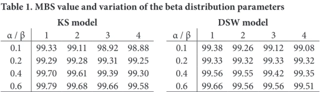
Table 1 represents sensitivities of the MBS prices towards the parameters of the beta distribution18. It can be observed that an increase in parameter α leads to an increase in the MBS value, while an increase in β has the inverse effect. 16 The probability density function of the beta distribution
is defined on the bounded set, which sets an upper bound for the transaction cost.
17 This is achieved by dividing the set [0,1] into N equal segments, and assuming the central point of each segment as representative for the corresponding class of borrowers. The respective transaction cost levels for each class of borrowers are obtained by applying the inverse of the cumulative distribution function to the central points.
18 The mean transaction cost is then given by α(α+β)-1, while variance is given by αβ(α+β)-2(α+β+1)-1. Note that we have chosen beta distribution (in line with DSW) such that α<1 and β≥1, for which its probability density function is strictly decreasing, implying a higher probability for the lower transaction costs. For comparison reasons, we use the parameters of the beta distribution as in DSW, namely, α=0.3779162, β= 2.8838.
An increase in β lowers the expectation and dispersion, resulting in a higher probability of lower transaction costs, which decreases the value of MBS. An increase in α increases both the expectation and dispersion and results in slightly higher transaction costs and thus higher MBS values.
Table 1. MBS value and variation of the beta distribution parameters
KS model DSW model α / β 1 2 3 4 α / β 1 2 3 4 0.1 99.33 99.11 98.92 98.88 0.1 99.38 99.26 99.12 99.08 0.2 99.29 99.28 99.31 99.25 0.2 99.33 99.32 99.33 99.32 0.4 99.70 99.61 99.39 99.30 0.4 99.56 99.55 99.42 99.35 0.6 99.79 99.68 99.66 99.58 0.6 99.66 99.56 99.56 99.51
Note: The calculations were done using the following parameters: contract rate 10.5%, servicing fee 0.5%, maturity 5 years, service flow 8.5%, initial spot rate 10%, steady-state spot rate 10%, interest rate st.dev. 10%, speed of adj. 0.25, house price volatility 10%, loan-to-value ratio 90%, assuming no correlation between the two Brownian motion processes and three levels of transaction costs. λ parameters for DSW model: β0=0.1, β1=1.5, β2=0.4, β3=1.1.
Sensitivity towards parameters inducing mortgage termination
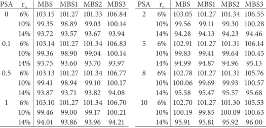
As mentioned above, termination in the KS model is induced by the probability of suboptimal termination which is projected in line with the PSA schedule.19 In Table 2 we observe that an increase in probability of suboptimal termination (an increase in PSA) lowers the value of MBS in the upward sloping yield curve environment, while when the yield curve is flat or downward sloping, the MBS value increases. This effect can be explained by more cash flows being returned to the investor due to suboptimal termination that, in the case of low interest rate levels, can be reinvested on less favourable terms (and vice-versa).
Table 2. MBS and mortgage asset values for different transaction costs in the KS model and variation of λ parameter
PSA r0 MBS MBS1 MBS2 MBS3 PSA r0 MBS MBS1 MBS2 MBS3 0 6% 103.15 101.27 101.33 106.84 2 6% 103.05 101.27 101.34 106.55 10% 99.35 98.89 99.03 100.14 10% 99.56 99.11 99.30 100.28 14% 93.72 93.57 93.67 93.94 14% 94.28 94.13 94.23 94.46 0.1 6% 103.14 101.27 101.34 106.83 5 6% 102.91 101.27 101.31 106.14 10% 99.36 98.90 99.04 100.14 10% 99.83 99.41 99.64 100.45 14% 93.75 93.60 93.70 93.97 14% 94.99 94.87 94.96 95.13 0.5 6% 103.13 101.27 101.34 106.77 8 6% 102.78 101.27 101.31 105.76 10% 99.41 98.94 99.10 100.17 10% 100.06 99.69 99.93 100.57 14% 93.87 93.71 93.82 94.08 14% 95.58 95.47 95.57 95.68 1 6% 103.10 101.27 101.34 106.70 10 6% 102.70 101.27 101.30 105.53 10% 99.46 99.00 99.17 100.21 10% 100.19 99.85 100.09 100.63 14% 94.01 93.86 93.96 94.21 14% 95.91 95.81 95.92 96.00
Note: The calculations were done using the following parameters: contract rate 10.5%, servicing fee 0.5%, maturity 5 years, service flow 8.5%, steady-state spot rate 10%, interest rate volatility 10%, speed of adj. 0.25, house price volatility 10%, loan-to-value ratio 90%, and no correlation. MBSi, i=1,2,3, are mortgage asset values for low, medium and high transaction costs.
Table 3. MBS and mortgage assets values for different transaction costs in the DSW model and variation in hazard rate parameters
β0 β2 β3 MBS MBS1 MBS2 MBS3 β0 β2 β3 MBS MBS1 MBS2 MBS3 0 0 -2 116.09 132.38 115.76 100.14 1 0 -2 109.90 123.38 108.35 97.97 -1 101.79 103.22 102.01 100.14 -1 99.88 102.41 99.25 97.97 0 100.14 100.14 100.14 100.14 0 98.65 100.08 97.90 97.97 1 99.76 99.51 99.62 100.14 1 97.63 97.39 97.53 97.97 2 99.62 99.30 99.42 100.14 2 97.54 97.27 97.38 97.97 0.5 -2 103.42 106.43 103.68 100.14 0.5 -2 101.04 104.72 100.42 97.97 -1 100.35 100.48 100.45 100.14 -1 98.83 100.38 98.13 97.97 0 99.82 99.60 99.72 100.14 0 97.67 97.45 97.60 97.97 1 99.66 99.38 99.47 100.14 1 97.57 97.30 97.42 97.97 2 99.54 99.17 99.33 100.14 2 97.47 97.13 97.31 97.97 1 -2 100.77 101.21 100.96 100.14 1 -2 99.12 100.89 98.50 97.97 -1 99.92 99.77 99.86 100.14 -1 98.49 99.81 97.70 97.97 0 99.69 99.40 99.52 100.14 0 97.58 97.31 97.46 97.97 1 99.56 99.20 99.36 100.14 1 97.49 97.16 97.34 97.97 2 99.51 99.12 99.27 100.14 2 97.44 97.09 97.27 97.97 Note: The calculations were done using the following parameters: contract rate 10.5%, servicing fee 0.5%, maturity 5 years, service flow 8.5%, initial spot rate 10%, steady-state spot rate 10%, interest rate volatility 10%, speed of adj. 0.25, house price volatility 10%, loan-to-value ratio 90%, and no correlation. Parameters λ for the DSW model are selected as follows: β1=1. MBSi, i=1,2,3, are mortgage asset values for low, medium and high transaction costs.
In the case of the DSW model, we observe that increased probability of suboptimal termination, either through the presence of background hazard rate or through increase in the values of parameters β2 and β3, lowers the value of MBS to the investor in the chosen economic environment. The same pattern can be observed in the case of mortgage assets for different levels of transaction costs.
We note that mortgage asset values for borrowers with high transaction costs remain unchanged if one varies parameters β2 and β3. This can be explained by high transaction costs that push both options out of money. As a result, mortgage termination is determined solely by the background hazard rate.
Sensitivity towards initial values of house price and interest rates
MBS value is affected in the same manner as the individual mortgage contract when it comes to the initial values of the underlying variables, as it is obtained by averaging the values of the single mortgage assets for different classes of borrowers. This can be seen by comparing the shape of MBS value with respect to different parameter values (Figure 1) and the shape of the mortgage liability value presented for borrowers of the lowest level of transaction costs (Figure 2).
Figure 1. Variation in the values of r0 and H0 of MBS value
Note: The calculations were done using the following parameters: contract rate 10.5%, servicing fee 0.5%, maturity 5 years, service flow 8.5%, steady-state spot rate 10%, speed of adj. 0.25, interest rate st.dev. 10%, house price st.dev. 10%, loan-to-value ratio 90%, no correlation, three levels of transaction costs. λ parameters for DSW model: β0=0.1, β1=1.5, β2=0.4, β3=1.1.
We observe that the rate at which MBS value changes with respect to different choices on initial parameter values differs in the two models, due to different triggers of mortgage termination. It can be observed that the change in underlying
variables has a higher impact on the endogenously induced termination, especially observed in the case of low initial values of house price.
The obtained shape is primarily governed by the interaction of the different components of the single mortgage contract. The mortgage value is driven by the combined effect of house price and interest rate levels on the present value of the remaining payments (PVRP) and the value of the two options. Low house price levels increase the option to default and thus decrease the mortgage value. With an increase in house price levels the prepayment option becomes more important. On the other hand interest rate level is the main driver of the values of both prepayment option and the present value of the remaining payments. These two quantities have an opposite impact on mortgage value. However as the prepayment option value is significantly lower than the PVRP, the interest rate effect on the mortgage value is mainly driven by the effect of interest rates on the PVRP.
Figure 2. Variation in the values of r0 and H0 of mortgage liability for borrower with the lowest transaction cost
Sensitivities towards loan-to-value ratio and interest rate and house price volatilities
As MBS value is obtained as the average of the values of mortgage assets for different transaction costs level, its sensitivity towards a parameter choice is derived from the sensitivity of the mortgage value. To give more insight as to how this value is generated we also include the values of mortgage liabilities in cases of different classes of borrowers. We observe that for each of the two models the value of mortgage liability rises with an increase in transaction costs. Higher transaction costs reduce the region where it is optimal to exercise the respective option and thus lower its value, which in turn raises the mortgage value.
Table 4. Variation in loan-to-value ratio and volatilities of the MBS and mortgage liability values for different transaction costs
KS model DSW model LTV σr σH MBS MBS1 MBS2 MBS3 MBS MBS1 MBS2 MBS3 0.8 0.05 0.05 99.9805 99.8038 101.2429 102.0546 99.6751 99.8821 100.8386 100.8479 0.1 99.9802 99.8031 101.2428 102.0546 99.6746 99.8807 100.8385 100.8479 0.2 99.7207 99.5685 101.0081 102.0161 99.6529 99.8591 100.8154 100.8455 0.1 0.05 99.4745 98.9975 100.9956 102.2151 99.4141 99.3420 100.7790 101.0231 0.1 99.4737 98.9957 100.9950 102.2151 99.4134 99.3390 100.7781 101.0231 0.2 99.2578 98.7944 100.7686 102.1686 99.3921 99.3186 100.7548 101.0199 0.2 0.05 98.7385 97.5885 100.0712 102.8222 99.0578 98.4805 100.3808 101.6847 0.1 98.7344 97.5808 100.0667 102.8224 99.0504 98.4750 100.3767 101.6847 0.2 98.5306 97.4189 99.8663 102.7440 99.0215 98.4535 100.3539 101.6782 0.9 0.05 0.05 99.9805 99.8038 101.2429 102.0546 99.6727 99.8573 100.8381 100.8479 0.1 99.9600 99.7844 101.2336 102.0542 99.6716 99.8552 100.8376 100.8479 0.2 98.9733 98.7067 100.3173 101.8905 99.5729 99.7631 100.7383 100.8361 0.1 0.05 99.4745 98.9975 100.9956 102.2151 99.4042 99.3019 100.7694 101.0231 0.1 99.4602 98.9812 100.9837 102.2148 99.4025 99.2988 100.7679 101.0231 0.2 98.5603 98.0242 100.0826 102.0247 99.3028 99.2213 100.6726 101.0083 0.2 0.05 98.7385 97.5885 100.0712 102.8222 99.0030 98.4138 100.3395 101.6847 0.1 98.7232 97.5695 100.0538 102.8216 98.9981 98.4061 100.3353 101.6847 0.2 97.8536 96.7632 99.2192 102.5329 98.9116 98.3372 100.2572 101.6580 1 0.05 0.05 99.6939 99.2968 101.2132 102.0533 99.6581 99.8196 100.8367 100.8479 0.1 99.1102 98.5141 100.7276 102.0436 99.6159 99.7678 100.8053 100.8478 0.2 96.8678 96.1167 98.3578 101.5045 99.3085 99.4814 100.4952 100.8025 0.1 0.05 99.2585 98.6789 100.9493 102.2138 99.3794 99.2574 100.7583 101.0231 0.1 98.7280 97.9614 100.4492 102.2025 99.3348 99.2151 100.7240 101.0230 0.2 96.5601 95.6410 98.1429 101.5995 99.0519 98.9557 100.4301 100.9691 0.2 0.05 98.5816 97.3958 100.0108 102.8209 98.9528 98.3429 100.3005 101.6847 0.1 98.1057 96.8177 99.5157 102.7962 98.9225 98.3071 100.2699 101.6838 0.2 95.9026 94.6806 97.3770 101.9666 98.6745 98.0868 100.0265 101.5980 Note: The calculations were done using the following parameters: contract rate 10.5%, servicing fee 0.5%, maturity 5 years, service flow 8.5%, initial spot rate 10%, steady-state spot rate 10%, speed of adjustment 0.25 and no correlation between the two sources of uncertainty. λ parameters for DSW model: β0=0.1, β1=1.5, β2=0.4, β3=1.1. MBSi, i=1,2,3 are mortgage liabilities values for low, medium and high transaction costs.
Higher volatility increases the probability of reaching the exercise region of the respective option and thus increases the value of the option and decreases the value of the mortgage. However this impact is offset by the competing effect of the other option. Furthermore the main driver of the mortgage value and of the
options values, PVRP, is directly affected by the change in σr20, while it is not affected by changes in values of σH or LTV.
It is also observed that increasing the LTV ratio decreases the value of the MBS, due to its direct effect on the default option value.
Sensitivities to the contract rate and LTV ratio
The MBS value increases in contract rate for all loan-to-value ratio levels. High values of loan-to-value ratio induce the default option to be deep in the money and it takes a small change to exercise it. As a result its value rises with an increase in LTV. A similar result holds for the prepayment option in the case of higher contract rates. This effect is transferred by averaging of the values of individual contracts to the value of MBS.
Figure 3. Variation in the values of c and LV of MBS value
Note: The calculations were done using the following parameters: servicing fee 0.5%, maturity 5 years, service flow 8.5%, steady-state spot rate 10%, speed of adj. 0.25, interest rate st.dev. 10%, house price st.dev. 10%, no correlation, three levels of transaction cost. λ parameters for DSW model: β0=0.1, β1=1.5, β2=0.4, β3=1.1.
It can be observed in the case of the KS model that for a fixed (higher) level of contract rate the MBS value increases to a certain point and then decreases, with an increase in LTV. This can again be explained by the behaviour of the options. The prepayment option value is in the money for the high value of contract rate. With increasing LVT, the default option increases and forces a decline in 20 This is due to the effect on the extent of the inverse relationship between interest rate and PVRP. The gains on interest rate decrease are higher than the losses on interest rate increase of the same magnitude, resulting in higher PVRP with increasing volatility.
the prepayment option value. The rising value of the default option forces the borrower to wait longer with the exercise of the prepayment option, inducing more monthly payments coming to the mortgage holder at a higher contract rate, leading to a higher mortgage value. However, when the LTV is sufficiently high, both options are deep in the money and the mortgage value drops due to the high probability of termination at favourable contract rates. For lower levels of contract rate, as the prepayment option is not in the money, this competing effect of options is largely offset. The increasing loan-to-value ratio increases the default option to a lesser extent resulting in an overall smaller decrease in the mortgage value at high values of LTV.
This behaviour is not observed in the DSW model, which is explained by its dependence on the exogenous termination, and inability to incorporate the interrelations of the underlying mortgage component in the various economic environments.
3.2. MBS pricing, duration and convexity
Table 5 represents prices, effective duration, and effective convexity for a hypothetical MBS with respect to the initial spot rate and the assumed set of parameters. It can be observed that the respective MBS is priced in line with expectations. For interest rate level near the coupon rate, the MBS is almost priced at par. For lower interest rate values, the respective MBS is priced as a premium security, while for higher interest rate levels it is priced as a discount. It can also be seen that MBS exhibits negative convexity21. The table demonstrates that both duration and convexity decrease with a lower level of interest rate, as prepayments then become more likely.
Table 5. MBS price, duration and convexity
KS model DSW model
r0 Price Duration Convexity r0 Price Duration Convexity
6% 103.10 0.67 36.18 6% 104.23 1.23 -2.31
8% 101.86 1.25 -82.98 8% 102.10 1.53 -30.23
10% 99.46 1.76 -13.66 10% 99.40 1.96 -24.79
12% 96.78 1.93 -13.80 12% 96.49 2.11 -2.23
14% 94.01 2.02 1.99 14% 93.58 2.18 4.07
Note: The calculations were done using the following parameters: contract rate 10.5%, servicing fee 0.5%, maturity 5 years, service flow 8.5%, steady-state spot rate 10%, interest rate volatility 21 This is a common characteristic of MBS, due to the opposite effect of prepayments and the
10%, speed of adjustment 0.25, house price volatility 10%, loan-to-value ratio 90%, and there are no correlation between the two sources of risk. Parameters λ for DSW model are: β0=0.1, β1=1.5, β2=0.4, and β3=1.1.
In order to quantify the influence of default option value on MBS valuation, we ran the simulations in a set up where the default option is excluded from the algorithm, meaning that the possible choices for the borrower are only continuation or prepayment. Frictions are included as before.
Table 6. MBS and mortgage assets values for different transaction costs with and without default option
KS model
with option to default without option to default
r0 MBS MBS1 MBS2 MBS3 r0 MBS MBS1 MBS2 MBS3 6% 101.310 99.689 99.822 104.420 6% 103.000 101.270 101.270 106.450 8% 100.130 99.060 99.450 101.870 8% 102.210 101.210 102.170 103.230 10% 98.214 97.624 97.774 99.244 10% 100.080 100.070 100.040 100.140 12% 95.912 95.545 95.611 96.580 12% 97.171 97.203 97.149 97.160 14% 93.478 93.238 93.277 93.920 14% 94.304 94.327 94.291 94.292 DSW model
with option to default without option to default
r0 MBS MBS1 MBS2 MBS3 r0 MBS MBS1 MBS2 MBS3 6% 104.100 102.940 103.160 106.210 6% 104.220 103.030 103.220 106.420 8% 102.220 101.750 102.060 102.850 8% 102.400 101.900 102.310 102.990 10% 99.475 99.437 99.377 99.610 10% 99.671 99.690 99.634 99.690 12% 96.413 96.413 96.352 96.476 12% 96.543 96.591 96.517 96.522 14% 93.420 93.426 93.380 93.454 14% 93.499 93.538 93.480 93.480 Note: The calculations were done using the following parameters: contract rate 10.5%, servicing fee 0.5%, maturity 5 years, service flow 8.5%, steady-state spot rate 10%, interest rate volatility 5%, speed of adjustment 0.25, house price volatility 20%, loan-to-value ratio 95%, and no correlation between the two sources of uncertainty. KS model: λ=2*PSA. λ parameters for DSW model: β0=0.1, β1=1.5, β2=0.4, β3=1.1. MBSi, i=1,2,3 are mortgage assets values for low, medium and high transaction costs.
Table 6 presents the results for the MBS value and mortgage asset value for the three different levels of transaction costs22 in the two scenarios - when default option is part of the valuation framework and when it is excluded. The parameter values were chosen to favour default – higher values of loan-to-value ratio and 22 Denoted by MBS1 that relates to borrowers of the lowest transaction const, MBS2 medium,
house price volatility. We see that exclusion of the default option raises the MBS value in the chosen economic environment in both models. The effect of MBS value increase is lower in the case of the DSW model, due to its lower ability to respond to underlying variables movements. It should be noted that the total value of the default option is understated, as its value is reduced when joined with the prepayment option. Equivalently, the prepayment option in the framework without the default option is overstated, as it does not compete with the default for value.
4. CONCLUSION
In this paper, we extend the work of Hilliard, Kau and Slawson (1998) and Kau and Slawson (2002) in order to value MBS securities. We do so by introducing the heterogeneity of borrowers in the manner of Downing, Stanton and Wallace (2003). Through various simulations we find that the models are flexible enough to capture most of the known features that MBSs exhibit.
It should be noted that the adopted approach is in a rather theoretical framework and no input parameters are calibrated to actual data, but are chosen in line with the presented literature. However, calibrating the model to the actual data would be one of the important extensions of this work, which could possibly lead to certain modifications.
The model aims to describe how the interaction of different components of the mortgage contract and economic environment affect MBS value. The presented models account for many different determinants of borrowers’ behaviour and are thus adaptive to different economic scenarios and can capture the influence of various exogenous factors. Furthermore, we have seen that the DSW model is less sensitive to the movements of the underlying variables due to its dependence on exogenous termination that is only partly connected to the underlying variables. As seen from the simulations, different components such as house price level, house price volatility, loan-to-value ratio, value of the prepayment option and its determinants (as prepaying leaves less opportunity for defaulting and vice versa), all affect default of the individual mortgage contract, and thus the value of the MBS. In certain economic environments the value of the default option is even larger than and more influential on the overall value of the mortgage than the prepayment option. The recent crisis seems to confirm this view.
Bardhan, A., Karapadža R. & Urošević, B. (2006). Valuing mortgage insurance contracts in emerging market economies. Journal of Real Estate Finance and Economics, 32(1), 9-20.
Cox J., Ingersoll, J. & Ross, S. (1985). A theory of term structure of interest rates. Econometrica, 53(2), 385-407.
Drenovak, M. & Urošević, B. (2010). Modelling the benchmark spot curve for the Serbian market.
Economic Annals, 55(184), 29-57.
Downing, C., Stanton, R. & Wallace, N. (2003). An empirical test of a two-factor mortgage valuation model: How much do house prices matter?. (Finance and Economics Discussions Series Working Paper No. 2003-42). Retrieved from the Board of Governors of the Federal Reserve System website: http://www.federalreserve.gov/pubs/feds/2003/200342/200342pap.pdf
Fabozzi, F. J. (2004). Fixed income analysis for the chartered financial analyst® program. 2nd Ed.
New Hope, PA: Frank J. Fabozzi Associates
Goncharov, Y. (2006). An intensity-based approach to the valuation of mortgage contracts and computation of the endogenous mortgage rate. International Journal of Theoretical and Applied Finance, 9(6), 889-914.
Hendershott, P. H. & Van Order, R. (1987). Pricing mortgages: an interpretation of the models and results.(NBER Working Paper No. 2290). Retrieved from the National Bureau of Economic Research website: http://www.nber.org/papers/w2290.pdf
Hillard, J.E., Kau, J.B. & Slawson, V.C. (1998). Valuing prepayment and default in a fixed-rate mortgage: A bivariate binomial options pricing technique. Journal of Real Estate Economic, 26(3), 431-468.
Hillard, J.E. & Schwartz, A. (1996). Binomial option pricing under stochastic volatility and correlated state variables. Journal of Derivatives, 4, 23-34.
Kalotay, A., Yang, D. & Fabozzi, F.J. (2004). An option-theoretic prepayment model for mortgages and mortgage-backed securities. International Journal of Theoretical and Applies Finance, 8, 949-978.
Kau, J.B. et al. (1992). A generalized valuation model for fixed-rate residential mortgages. Journal of Money, Credit and Banking, 24(3), 279-299.
Kau, J.B. & Keenan, D.C. (1995). An overview of the option-theoretic pricing of mortgages. Journal of Housing Research, 6(2), 217-244.
Received: September 28, 2010 Accepted: October 27, 2010 Kau, J.B. & Slawson, V.C. (2002). Frictions, heterogeneity and optimality in mortgage modelling.
Journal of Real Estate Finance and Economics. 24(3), 239-260.
Kolbe, A. (2007). Valuation of mortgage products with stochastic prepayment-intensity models. Technische Universität München
Longstaff, F.A. (2002). Optimal recursive refinancing and the valuation of mortgage-backed securities. Retrieved from the eScholarship Repository, University of California website: http:// escholarship.org/uc/item/19k7479t
Nelson, D.B. & Ramaswamy, K. (1990). Simple binomial processes as diffusion approximations in financial models. Review of Financial Studies, 3(3), 393-430.
Richard, S.F. & Roll, R. (1989). Prepayments on fixed-rate mortgage-backed securities. Journal of Portfolio Management, Spring 1989, 73-82.
Schwartz, E.S. & Torous, W.N. (1989). Prepayment and valuation of mortgage-backed securities.
The Journal of Finance, 44(2), 375-392.
Schwartz, E.S. & Torous, W.N. (1992). Prepayment, default and the valuation of mortgage pass-through securities. The Journal of Business, 65(2), 221-239.
Salomon Smith Barney. (2001). Guide to mortgage-backed and asset-backed securities, New York: John Wiley & Sons.
Spahr, R.W. & Sunderman, M.A. (1992). The effect of prepayment modelling in pricing mortgage-backed securities. Journal of Housing Research, 3(2), 381-400.
Stanton, R. (1995). Rational prepayment and the valuation of mortgage-backed securities. Review of Financial Studies, 8, 677-708.