Troubled Banks: Why Don t They All Fail?

(1)

by Robert Oshinsky and Virginia Olin*

A wealth of literature examines the determinants of bank failures and of bank mergers or consolida-tions. Also numerous are studies that develop fail-ure-prediction models and early-warning systems. But both groups of studies use samples of all banks, and therefore most of this research focuses on pairs of outcomes: failure versus nonfailure, merger ver-sus consolidation,1_{or problem bank versus} non-problem bank. But in reality, future status is more than a binary choice.

Here we study only troubled banks—banks that receive a composite CAMELS rating of either 4 or 5 when examined.2 _{A focus on troubled banks is} valuable to the FDIC and bank researchers for four reasons. First, when a bank is troubled, failure is but one possible outcome; alternative outcomes are recovery, merger, or continuation as a problem. Second, between 1990 and 2002, 96 percent of all banks that failed had first been troubled banks. Including nonproblem banks would add bias towards non-failure as a possible outcome since a vast majority of nonproblem banks do not fail. Third, if the FDIC can better predict the number of troubled banks that will not fail, it will be better able to estimate the size of its contingent loss reserve.3 _{Finally, development of a multistate} model identifying financial characteristics that

contribute to recovery as well as to failure is important for the FDIC’s long-term strategic plan-ning: accurate predictions of the future states of problem banks would affect the resources applied to these banks.

* Robert Oshinsky is a Senior Financial Economist and Virginia Olin is a former Senior Financial Economist, Division of Insurance and Research, Federal Deposit Insurance Corporation (FDIC). The authors thank John O’Keefe for his overall guidance; Andrew Davenport for his counsel; and Jesse Weiher, Brian Lamm, James Marino, and the anonymous readers of the FDIC for their careful review of the article and their valuable comments and suggestions. The authors also thank Robert DeYoung for his suggestions. Of course, all mistakes are the responsibility of the authors. The views expressed here are those of the authors and not necessarily those of the FDIC.

1_{In previous studies, a merger is the absorption of a bank by a previously}

unrelated bank while consolidation is the absorption of a bank by a related bank. For purposes of this paper, we combine the two types of absorptions and refer to them as mergers.

2 _{Because of the nature of the resolution process, we deliberately omit}

troubled thrifts, including those resolved by the Resolution Trust Corporation, which kept insolvent thrifts open during the resolution process.

CAMELS is an acronym for the six components of the regulatory rating system: Capital adequacy, Asset quality, Management, Earnings, Liquidity, and (since 1998) market Sensitivity. Banks are rated from 1 (the best) to 5 (the worst), and banks with a composite rating of 4 or 5 are considered problem banks. A rating of 4 generally indicates that the bank exhibits unsafe or unsound practices or is in an unsafe or unsound condition, while a rating of 5 means that the bank’s practices or condition are extremely unsafe or unsound.

3 _{The mission of the FDIC is to protect depositors and promote the safety}

and soundness of insured depository institutions and the U.S. financial system by identifying, monitoring, and addressing risks to the deposit insurance funds. The FDIC’s Financial Risk Committee quantifies risks to the deposit insurance system for purposes of financial reporting and fund management, and each quarter it meets to set a contingent loss reserve estimated from total assets of banks that may fail within two years.

(2)

Troubled Banks: Why Don’t They All Fail?

As noted, troubled banks have four possible out-comes: recovery, merger, continuation as a prob-lem, and failure. Knowing the future states of banks in our sample,4_{we construct a financial} pro-file using pre-examination data for the banks grouped by their future state and then use these profiles to develop a multinomial logit estimating procedure that predicts a bank’s likely future state. We show that a four-state model predicts failure at least as well as binary failure-prediction models and, in addition, provides predictive ability for three alternative future states.

The next section describes previous empirical stud-ies of bank failures, mergers, and financial distress. The three subsequent sections discuss the method-ology we use, the sample and data, and the results. The concluding section gives a brief summary.

Empirical Studies

Most of the numerous studies that examine the determinants of bank failures and bank mergers and consolidations, like most of the numerous studies that develop early-warning systems predict-ing deterioration in banks’ financial condition, construct financial ratios based on information in the Consolidated Reports of Condition and Income (Call Reports) that banks file quarterly with the FDIC.5 _{The idea is to construct financial} ratios that closely resemble the CAMELS rating system used by bank examiners and to use the ratios to predict pairs of outcomes: failure versus nonfailure, merger versus consolidation, or prob-lem bank versus nonprobprob-lem bank.6 _{While the} information used by examiners is preferable, it is not available without an examination, unlike Call Report data, which are readily available quarterly. Only a few studies have extended this research beyond pairs of outcomes. In an effort to improve predictive accuracy, DeYoung estimates the long-run probability of failure and acquisition in de novo banks by defining three states: failure, merger by acquisition, and conversion of a whole-bank affiliate of a bank holding company to a branch bank of that same bank holding company.

Wheelock and Wilson use a competing-risks model to consider the joint determination of the proba-bility of being acquired, failing, or surviving. Han-nan and Rhoades predict that a bank may

experience one of three outcomes: not be acquired, be acquired by a firm operating within the bank’s market, or be acquired by a firm operating outside the bank’s market.7 _{DeYoung expects that} includ-ing the other two exit states (merger by acquisi-tion, and conversion) will make the failure estimates more accurate. Wheelock and Wilson find that inefficiency increases the risk of failure while reducing the probability of a bank’s being acquired. And Hannan and Rhoades find that adding the third state (distinguishing between types of mergers) yields a number of firm and mar-ket characteristics that earlier studies did not yield and that significantly influence the likelihood of acquisition.

Rarely in life are the possible outcomes binary. While studies that examine two-state outcomes have benefit, much is lost by not studying other possible outcomes. Further, by limiting our uni-verse to only problem banks, we are able to remove the inherent bias towards the prediction of non-failure status.

Methodology

Referencing previous studies, we select certain financial variables proven in binary models to be useful in determining future bank state. In our multistate model we use univariate trend analysis to determine whether prior-period financial char-acteristics differ by future bank state.

Specifically, in the existing literature on bank per-formance the reasons suggested for failure include 4 _{Our sample consists of institutions assigned a CAMELS rating of 4 and 5}

between 1990 and 2002. The sample is described in detail in a later section of this article.

5 _{For reviews of the literature, see Demirgüç-Kunt (1989), Jagtiani et al.}

(2003), and King et al. (2005).

6 _{See Whalen (1991), Cole and Gunther (1998), Kolari et al. (2002), and}

Jagtiani et al. (2003).

7 _{DeYoung (2003), Wheelock and Wilson (2000), and Hannan and Rhoades}

(3)

low capital, risky asset portfolios, poor manage-ment, low earnings, and low liquidity. Thus, the financial variables we select are from those same broad categories: capital adequacy, asset quality, management, earnings, and liquidity. In addition, we run a one-way analysis of variance to examine the financial characteristics of recovered banks versus banks in the other three states (merged or acquired, remained a problem, and failed).

We use a multinomial logistic estimating procedure to model future bank state. Outcomes are nomi-nal, and therefore the multinomial logit model’s assumptions are the closest fit to the specification of the model being estimated. This model simulta-neously estimates three binary logits for pairwise comparisons among the outcome categories to a reference outcome. These binary logits are (1) recover relative to failure, (2) merge relative to failure, and (3) remain a problem relative to fail-ure.

A general form of the model tested is shown in equation 1, where Probability of State (k)_i,tis the probability that bank iwill be in state kat time t. (1) Probability of State (k)_i,t=

(1) F(Financial condition_i,t-1, Economic conditions_t)

We gauge the model’s effectiveness in several ways. First, we compare the out-of-sample forecasting accuracy for each of the four states with the actual number of banks ending up in each state. We compare two competing binary models with the multistate model for failure predictions: one of the two competing models uses the same variables that our multistate model uses, and the other uses the same explanatory variables that Jarrow et al. use, referred to as the loss-distribution model.8 _These two comparisons allow us to test whether including additional alternative states improves the accuracy of failure estimates over the accuracy of binary models. Second, we investigate the economic and statistical effect of our explanatory variables. Third, we check to determine that the banks with the highest predicted probability of failure from our model are the ones that actually fail.

Sample and Data

Our sample consists of 1,996 banks on the FDIC problem-bank list from 1990 through 2002. Each bank has at least one first event and second event that are paired as an observation. The first event occurs when a bank is examined and receives a CAMELS rating of 4 or 5. The second event occurs when the bank does one of the following: recovers (improves to a CAMELS rating of 1, 2, or 3 at the next examination), merges (either merges with a bank outside of its multibank holding com-pany or consolidates within its multibank holding company),9_{remains a problem bank (continues to} have a CAMELS rating of 4 or 5 at the next examination), or fails.10 _{We use only observations} in which first events are paired with second events that occurred 6 to 24 months after the first events. Any second events sooner than 6 months or later than 24 months are ignored, and the observation is dropped from the sample. The reason for this restriction is twofold: first, we want to allow enough time to pass for changes in financial condi-tion to occur; second, during most of our period, all banks except those with assets under $250 mil-lion and a composite CAMELS rating of 1 or 2 were required by law to receive safety-and-sound-ness examinations annually.11 _{As noted above, a} pairing of events is considered one observation in our sample. Our sample consists of 3,747 observa-tions.

To control implicitly for the effects of economic conditions and banking legislation, we divide these 3,747 observations into annual cohorts correspon-ding to the year of the first event. But because second events usually occur in a different year from the first events, we recognize that using annual

8 _{Jarrow et al. (2003).}

9 _{We recognize that mergers and consolidations have different characteristics.}

However, during the period we study, the number of consolidations is small (39), so we combined both events into one state.

10 _{Here we define failure either as a closing that results from an action by a}

regulator or as a merger assisted by the FDIC.

11 _{The frequency of examinations was set by the Federal Deposit Insurance}

Corporation Improvement Act of 1991 (FDICIA). Further exceptions to the requirement for annual safety-and-soundness exams are listed in the act.

(4)

Troubled Banks: Why Don’t They All Fail?

cohorts does not completely control for these effects.

A bank appears as an observation in a cohort only once, and each observation belongs to only one cohort.12 _{All observations end with the} occur-rence of the second event. If the bank in a given cohort reaches the second event as recovered (or merged, or a continued problem), the outcome for the observation for that bank in the cohort is con-sidered a recovery (or a merger, or continuation as a problem).

The same bank can be an observation in multiple cohorts depending on when it first receives a CAMELS rating of 4 or 5 and on its outcome at the second event. If, at the second event, the bank upon reexamination continues as a problem bank, the first observation ends with an outcome of continuation as a problem bank, and concur-rently a second observation for that bank begins and is paired with its corresponding subsequent event, which takes place 6 to 24 months later. At this subsequent event, an outcome is determined for that second observation. In contrast, when a bank’s first observation ends with a second event of recovery or merger, the bank has no concurrent second observation since it is no longer a problem bank. However, recovered banks may reemerge in our sample in a later cohort (for example, the bank recovers but later reverts to problem-bank status), whereupon the bank would be considered a new observation. Banks cannot appear in cohorts after they fail or merge.

Our sample has the following characteristics: The number of problem banks declines drastically dur-ing the 1990s as the bankdur-ing crisis that began in the mid-1980s and lasted through the early 1990s subsided. As figure 1 shows, the 1991 cohort has the highest number (897) and the 1997 cohort the lowest (62). Figure 2 shows that the 1990 and 1998 cohorts have the highest percentage of prob-lem banks that fail—5 percent—and that in the 1997 and 2002 cohorts, no problem banks fail before the second event. Throughout the period most banks remain a problem at the second event: the range is from a high of 69 percent in the 1990 cohort to a low of 40 percent in the 1997 cohort,

with an average of 49 percent. The proportion that merge by the second event is small, ranging from 3 percent in the 1990 cohort to 20 percent in the 1998 cohort. The proportion that recover by the second event ranges from a low of 23 percent in the 1990 cohort to a high of 53 percent in the 1997 cohort (figure 2). Moreover, for banks that recovered we found that large increases in internal capital injections (as a percentage of average assets) peaked in 1996. For those banks, external capital injections increased sharply from 1994 to 1995 but did not peak until 1999 (figure 3).13 Fig-ure 4 shows that most banks that remain a problem at the second event ultimately recover.14

Using data from the Call Reports, we calculate beginning and ending event financial ratios for each bank. The beginning event ratios are calcu-lated from the Call Report filed just before the first event and the one filed 12 months previously.15 Balance-sheet items are averaged for the two reporting periods and taken as a ratio of average assets for the same two periods; income items are summed over the 12-month period and taken as a percentage of average assets for the two periods. Similar calculations are made for the ending event, using the Call Report filed immediately before the second event and the one filed 12 months previ-ously.

We group banks by future state to compare their condition and performance. We then compare data reported at the ending period with those reported at the beginning. We compute the per-centage of banks in each state that showed an 12 _{Technically a bank may appear as a second observation in the same cohort}

since the window for the second event is as short as six months.

13 _{Jones and Critchfield (2004) note three reasons that might explain the 1997}

and 1998 peak years for merger activity and recoveries: (1) banks were highly profitable, liquid, and operating in favorable economic and interest-rate environments; (2) in 1994 the Riegle-Neal Interstate Banking and Branching Efficiency Act removed the remaining barriers to interstate banking and branching; and (3) a record-breaking bull market in stocks pushed market valuations of banks and thrifts to unprecedented levels, encouraging many banking firms to use their stock as currency to purchase other firms.

14 _{The reason for the decline beginning in 2001 in the percentage of}

still-a-problem banks that ultimately recover is that enough follow-up events have not yet occurred. Most banks remain a problem beyond a second event.

15 _{Gunther and Moore (2000) find atypical movements in Call Report data for}

the quarters in which banks are downgraded by examiners. These Call Reports are more subject to revisions. For that reason, we also did our univariate analysis on the Call Reports filed before the ones specified in this article. The resulting trends in data were similar to the trends reported here.

(5)

increase between the two periods for each of the financial ratios. Assuming that banks that recover are able to improve net income and net noninter-est income more than those that fail, we expect to see that the percentages of banks with increases in such ratios will be greater for banks having a future state of recovery than for banks with a future state of failure. For expense items, we expect the oppo-site. Assuming that banks that recover shed non-performing and past-due assets, we expect that the percentages of banks with increases in such assets will be less for banks that recover than for those that fail. We expect that the percentages of banks with increases in volatile liabilities and illiquid assets will be smaller for banks having a future state of recovery than for banks with a future state of failure and that the percentages of banks with

increases in capital will be larger for banks that recover than for those that fail. For the various financial ratios, we have no expectations for the ranking of banks that merge or are still a problem except that their increases or decreases will fall between the levels for banks that recover and banks that fail.

For measures of earnings, we compare the percent-age of banks in each state that showed increases in net interest income, in net noninterest income, and in provision for loan losses. For measures of risky asset portfolios, we compare the percentage of banks in each state that showed increases in aver-age allowance for loan and lease losses, averaver-age loans and leases past due 30–89 days, average loans and leases past due 90 days or more, average

866 897 713 413 194 110 64 62 65 76 74 98 115 1990 1991 1992 1993 1994 1995 1996 1997 1998 1999 2000 2001 2002 0 200 400 600 800 1000 Number of Banks Figure 1

Number of Troubled Banks by Cohort

1990 1991 1992 1993 1994 1995 1996 1997 1998 1999 2000 2001 2002 0

2 4 6

Percent of Average Assets

0 20 40 60 Percent of Banks that Recovered

External Injections Internal Injections

Note: 12 months before recovery.

Figure 3

External and Internal Capital Injections in Troubled Banks That Recovered

1990 1991 1992 1993 1994 1995 1996 1997 1998 1999 2000 2001 2002 0 20 40 60 80 100 Percent Recover Merge Remain a Problem Fail Figure 2

Cohort Composition of Troubled Banks at Second Event 595 535 359 190 87 52 ₃₂ 25 27 36 35 47 57 1990 1991 1992 1993 1994 1995 1996 1997 1998 1999 2000 2001 2002 0 200 400 600

Number of Troubled Banks

0 20 40 60 80 100 Percent of Banks that Recovered

Number of Troubled Banks Percent that Ultimately Recovered

Figure 4

Number of Troubled Banks That Remain a Problem and Ultimately Recover

(6)

Troubled Banks: Why Don’t They All Fail?

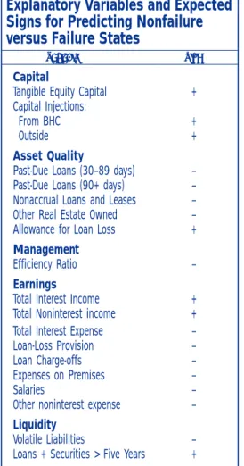
nonaccrual loans and leases, and average other real estate owned. For measures of capital adequacy we compare the percentage that showed average risk-based capital and average tangible equity capital; for measures of liquidity, the percentage that showed average volatile liabilities and loans and securities with maturities greater than or equal to five years. And for the management measure, we use the efficiency ratio (noninterest expense as a percentage of net interest income plus noninterest income). A lower efficiency ratio is better. To model future bank states, we selected almost the same financial variables that we used in the univariate trend analysis.16 _{For measures of the} economy, we added capital injections from a bank holding company and capital injections from out-side.17 _{From the univariate trend analysis we are} able to form expectations about the sign that coef-ficients on these variables will take when they are estimated by logit analysis. A negative coefficient implies that an increase in the variable will result in the future state’s becoming less likely relative to failure. A positive coefficient implies the opposite. Table 1 shows the expected sign of explanatory variables used in the multistate model. The finan-cial ratios associated with not failing are capital, capital injections, allowance for loan losses, inter-est income, noninterinter-est income, and longer-term assets (assets and securities with maturities equal to or great than five years). Although we expect a negative sign for the efficiency ratio’s coefficient (because lower is better), we associate this ratio, too, with not failing. The financial ratios associat-ed with failure are those measuring poor asset qual-ity (past-due loans, nonaccruing loans, and real estate owned), expense items (interest expense, loss provision, loan charge-offs, salaries, expenses on premises, and other noninterest expense), and volatile liquidity as measured by volatile

liabilities.18

Results

Our results from both the univariate trend analysis and the multistate logit estimating procedure gen-erally agree with expectations. Of banks that recover, the percentage with increases (between the beginning and ending periods) in performance

ratios such as net income and net noninterest income is greater than the percentage of banks in any alternative state. For loan-loss provisions, the opposite occurs. In addition, the percentage of banks that have increases in any of the risky asset measures is smaller for banks that recover than for banks in any alternative state. These results can be seen graphically in the appendix.

Explanatory Variables and Expected

Signs for Predicting Nonfailure

versus Failure States

V

Vaarriiaabbllee SSiiggnn Capital

Tangible Equity Capital +

Capital Injections:

From BHC +

Outside +

Asset Quality

Past-Due Loans (30–89 days) –

Past-Due Loans (90+ days) –

Nonaccrual Loans and Leases –

Other Real Estate Owned –

Allowance for Loan Loss +

Management

Efficiency Ratio –

Earnings

Total Interest Income +

Total Noninterest income +

Total Interest Expense –

Loan-Loss Provision –

Loan Charge-offs –

Expenses on Premises –

Salaries –

Other noninterest expense –

Liquidity

Volatile Liabilities –

Loans + Securities > Five Years +

Table 1

16 _{For the logits we used total income and detailed expense items instead of}

net interest and net noninterest income as used in the univariate analysis. In addition, we also estimated the model using Call Report data from the quarter before the quarter that precedes the examination, as in the univariate. The results differed little from those reported here.

17 _{As pointed out in footnote 13, the economy (a record-breaking bull market)}

was one reason noted for increased acquisitions.

18 _{Volatile liabilities are defined in the FDIC data dictionary as (1) federal}

funds purchased and sold under agreements to repurchase, (2) demand notes issued to the U.S. Treasury and other borrowed money, (3) time deposits over $100,000 held in domestic offices, (4) foreign-office deposits, (5) trading liabilities less trading liabilities’ revaluation losses on interest rate, (6) foreign exchange rate, and (7) other commodity and equity contracts.

(7)

In the logit analysis, we find that increases in financial ratios associ-ated with nonfailure have positive coefficients, and increases in finan-cial ratios associated with failure have negative coefficients.

Analysis of Variance

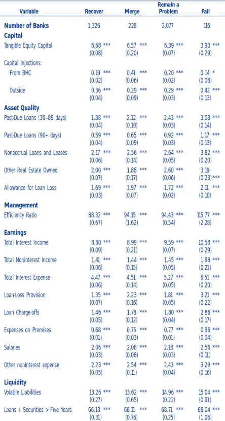
Results from the analysis of vari-ance, reported in tables 2 and 3, complement the results of the uni-variate trend analysis. Both tables use the beginning-period data. Table 2 shows the mean and stan-dard errors for financial variables in each of the four states. Table 3 shows the differences in means and statistical significances for six pair-ings: (1) recover versus merge, (2) recover versus remain a problem, (3) recover versus fail, (4) remain a problem versus merge, (5) remain a problem versus fail, and (6) merge versus fail.

The results reported in table 2 show that at the first event, the mean value for each financial vari-able is statistically different from zero. The results also show that the mean values in financial ratios associated with not failing are gen-erally larger for banks that recover, merge, or remain a problem than for banks that fail. The opposite is true for the mean values in finan-cial ratios associated with failing. There are three exceptions, how-ever: the mean values for total interest income, total noninterest income, and loans and securities with maturities greater than or equal to five years are largest for banks that fail. These results seem counterintuitive until we consider that banks with a future state of

Table 2

Mean and Standard Errors for Financial Variables, by State

(Standard Errors in Parentheses)

Remain a

Variable Recover Merge Problem Fail

Number of Banks 1,326 228 2,077 116

Capital

Tangible Equity Capital 6.68 *** 6.57 *** 6.39 *** 3.90 ***

(0.08) (0.20) (0.07) (0.29) Capital Injections: From BHC 0.19 *** 0.41 *** 0.20 *** 0.14 * (0.02) (0.06) (0.02) (0.08) Outside 0.36 *** 0.29 *** 0.29 *** 0.42 *** (0.04) (0.09) (0.03) (0.13) Asset Quality

Past-Due Loans (30–89 days) 1.88 *** 2.12 *** 2.43 *** 3.08 ***

(0.04) (0.10) (0.03) (0.14)

Past-Due Loans (90+ days) 0.59 *** 0.65 *** 0.92 *** 1.17 ***

(0.04) (0.09) (0.03) (0.13)

Nonaccrual Loans and Leases 2.17 *** 2.56 *** 2.64 *** 3.82 ***

(0.06) (0.14) (0.05) (0.20)

Other Real Estate Owned 2.00 *** 1.88 *** 2.60 *** 3.19

(0.07) (0.17) (0.06) (0.23) ***

Allowance for Loan Loss 1.69 *** 1.97 *** 1.72 *** 2.11 ***

(0.03) (0.07) (0.02) (0.10)

Management

Efficiency Ratio 88.32 *** 94.15 *** 94.43 *** 115.77 ***

(0.67) (1.62) (0.54) (2.28)

Earnings

Total Interest Income 8.80 *** 8.99 *** 9.59 *** 10.58 ***

(0.09) (0.21) (0.07) (0.29)

Total Noninterest income 1.41 *** 1.44 *** 1.45 *** 1.98 ***

(0.06) (0.15) (0.05) (0.21)

Total Interest Expense 4.47 *** 4.51 *** 5.27 *** 6.51 ***

(0.06) (0.14) (0.05) (0.20) Loan-Loss Provision 1.35 *** 2.23 *** 1.81 *** 3.21 *** (0.07) (0.16) (0.05) (0.22) Loan Charge-offs 1.46 *** 1.78 *** 1.80 *** 2.86 *** (0.05) (0.12) (0.04) (0.17) Expenses on Premises 0.68 *** 0.75 *** 0.77 *** 0.96 *** (0.01) (0.03) (0.01) (0.04) Salaries 2.06 *** 2.08 *** 2.18 *** 2.56 *** (0.03) (0.08) (0.03) (0.11)

Other noninterest expense 2.23 *** 2.54 *** 2.43 *** 3.29 ***

(0.05) (0.11) (0.04) (0.16)

Liquidity

Volatile Liabilities 13.26 *** 13.62 *** 14.96 *** 15.04 ***

(0.27) (0.65) (0.22) (0.91)

Loans + Securities > Five Years 66.13 *** 68.11 *** 68.71 *** 68.04 ***

(0.31) (0.76) (0.25) (1.06)

(8)

Troubled Banks: Why Don’t They All Fail?

Table 3

Differences in Means and Standard Errors of Financial Variables for Selected Pairs

(Standard Errors in Parentheses)

Recover- Merge Remain a

Recover Remain a Recover- Remain a Problem Merge

Variable Merge Problem Fail Problem Fail Fail

Capital

Tangible Equity Capital 0.10 0.29 ** 2.78 *** 0.19 2.49 *** 2.68 ***

(0.22) (0.11) (0.30) (0.22) (0.29) (0.35) Capital Injections: From BHC -0.22 *** (0.01) 0.04 0.21 *** 0.05 0.26 ** (0.06) (0.03) (0.08) (0.06) (0.08) (0.10) Outside 0.07 0.08 (0.06) 0.00 -0.14 -0.13 (0.10) (0.05) (0.13) (0.10) (0.13) (0.16) Asset Quality

Past-Due Loans (30–89 days) -0.24 ** -0.55 *** -1.20 *** -0.31 ** -0.65 *** -0.96 ***

(0.11) (0.05) (0.15) (0.11) (0.15) (0.18)

Past-Due Loans (90+ days) -0.06 -0.33 *** -0.58 *** -0.27 ** -0.25 * -0.52 ***

(0.10) (0.05) (0.13) (0.10) (0.13) (0.16)

Nonaccrual Loans and Leases -0.39 ** -0.47 *** -1.65 *** -0.09 -1.18 *** -1.27 ***

(0.15) (0.07) (0.20) (0.15) (0.20) (0.24)

Other Real Estate Owned 0.12 -0.59 *** -1.19 *** -0.72 *** -0.59 ** -1.31 ***

(0.18) (0.09) (0.24) (0.18) (0.24) (0.29)

Allowance for Loan Loss -0.29 *** -0.04 -0.42 *** 0.25 ** -0.38 *** -0.13

(0.08) (0.04) (0.11) (0.08) (0.11) (0.13)

Management

Efficiency Ratio -5.83 *** -6.10 *** -27.44 *** -0.28 -21.34 *** -21.62 ***

(1.76) (0.86) (2.37) (1.71) (2.34) (2.79)

Earnings

Total Interest Income -0.19 -0.79 *** -1.78 *** -0.60 ** -0.99 *** -1.59 ***

(0.22) (0.11) (0.30) (0.22) (0.30) (0.36)

Total Noninterest income -0.03 -0.04 -0.57 ** -0.01 -0.53 ** -0.54 **

(0.17) (0.08) (0.22) (0.16) (0.22) (0.26)

Total Interest Expense -0.03 -0.79 *** -2.03 *** -0.76 *** -1.24 *** -2.00 ***

(0.15) (0.07) (0.21) (0.15) (0.20) (0.24) Loan-Loss Provision -0.88 *** -0.46 *** -1.85 *** 0.42 ** -1.40 *** -0.97 *** (0.17) (0.08) (0.23) (0.17) (0.23) (0.27) Loan Charge-offs -0.32 ** -0.33 *** -1.39 *** -0.02 -1.06 *** -1.08 *** (0.13) (0.07) (0.18) (0.13) (0.18) (0.21) Expenses on Premises -0.07 ** -0.09 *** -0.28 *** -0.02 -0.19 *** -0.21 *** (0.03) (0.02) (0.04) (0.03) (0.04) (0.05) Salaries -0.03 -0.12 ** -0.50 *** -0.09 -0.38 *** -0.48 *** (0.08) (0.04) (0.11) (0.08) (0.11) (0.13)

Other non-interest expenses -0.30 ** -0.20 *** -1.06 *** 0.11 -0.86 *** -0.76 ***

(0.12) (0.06) (0.16) (0.12) (0.16) (0.19)

Liquidity

Volatile Liabilities -0.36 -1.70 *** -1.78 * -1.34 * -0.09 -1.43

(0.70) (0.35) (0.95) (0.69) (0.94) (1.12)

Loans + Securities > Five Years -1.98 ** -2.57 *** -1.91 * -0.60 0.66 0.07

(0.82) (0.40) (1.11) (0.80) (1.09) (1.31)

(9)

fail probably take on riskier assets that will have higher yields than banks with one of the alterna-tive future states. Or, turning the statement around, we can say that banks with riskier assets have a higher probability of failure. Fee income from these riskier assets may have resulted in high-er noninthigh-erest income. And in banks with a future state of fail, the ratio between loans and securities in the longer-term assets may be geared toward loans that are usually considered riskier than more-liquid securities.

The results reported in table 3 show that except for two variables (capital injections from the bank holding company and from outside), the difference in means between banks that recover and those that fail is statistically significant. Also significant for most variables are the differences in means between banks that fail and both banks that merge and banks that remain a problem.

The results from table 3 indicate as well that the differences in means between banks that remain a problem and both banks that merge and banks that recover are statistically significant. For the recovery-versus-merger pairing, fewer variables are statistically different from one another. And for the pairing remain-a-problem versus merge, even fewer variables are statistically different from one another.

Logit Analysis

For our multivariate analysis, we rely on a multino-mial unordered logit probability model that takes into account all four future bank states. Equation 2 shows the model tested:

(2) Probability of State (k)_i,t=

(2) F(Financial condition_i,t-1)

For a number of reasons, we did not include vari-ables for economic condition in our model. First, Nuxoll et al. found that state and local economic data did not contribute to the performance of stan-dard off-site models.19 _{Second, much of the} litera-ture theorizes that the economy is subsumed in the balance sheet, so any effect of the economy will

already have shown up in the financial data.20 Finally, we included capital injections as a proxy for changes in the economy (see footnote 13). We used a stepwise logit estimation procedure to identify the terms that have a significant relation-ship in predicting the likelihood that a bank will end up in one of the four states. The stepwise esti-mation procedure allows us to include several measures of the same attribute in the logit model, yet isolates the most important factors in terms of predicting future bank state.

Table 4 shows summary statistics for the variables used in the logistic regressions. The beginning-period data, as explained in the section on sample and data, are used in this table.21 _{We estimate the} logits for each of our cohorts, 1990 through 2002. However, because of the small number of failures after 1993, beginning with the 1994 logit we com-bine cohorts. The 1994 model is a combination of the 1993 and 1994 cohorts, and the 1995 model combines 1993 through 1995. We continue com-bining cohorts up to five years (the 1993 through 1997 cohorts for the 1997 logit). For the 1998 through 2002 models, we use a panel of the most recent previous five years.

Tables 5 through 7 show the results. The reference state is failure, so the coefficients are interpreted relative to failure. As mentioned above, a nega-tive coefficient means that an increase in a vari-able will have the result that the future state relative to failure becomes less likely.

19 _{Nuxoll et al. (2003).}

20 _{As a robustness check, we estimated the model using three variables for}

the United States economy: a ratio of the number of problem banks to total number of banks by state, a ratio of the assets of problem banks to total assets by state, and the percentage change in state housing permits. The first test was an estimation using only the economic variables as explanatory variables. We did two estimations: one used the ratio of the number of problem banks to total number by state and the percentage change in state housing permits; the second used the ratio of the assets of problem banks to total assets by state and the percentage change in housing permits. These variables were significant for most of these estimations. However, when these variables were included in estimations with the rest of the explanatory variables, their significance disappeared.

21 _{As with the univariate analysis, we also ran the logits using a beginning}

period one quarter before the quarters specified previously. The results revealed little difference.

(10)

Troubled Banks: Why Don’t They All Fail?

Eight of the findings are fairly interesting. First, more recent cohorts (beginning with the 1995–1999 cohort) have fewer statistically significant vari-ables than those in the early 1990s. This result is most likely because of the small number of failures, despite the paneling of data.22 _However, those variables that are statis-tically significant in the more recent cohorts have the expected sign (as shown in table 1) except for capital injections. For example, in the 1997–2001 cohort,

expenses on premises is signifi-cant and has a negative sign in table 5 (recovery) and table 7 (still a problem). An increase in this variable will have the result that a future state of either recovery or continua-tion as a problem becomes less likely relative to failure. On the other hand, for the cohorts 1994–1998 through 1998–2002, capital injections from outside are significant— but have the unexpected sign both for table 6 (merger) and, in two of those four cohorts, for table 5 (recovery). Perhaps the negative sign indicates that the institution expects to be acquired and either does not or cannot raise capital. As mentioned in footnote 13, the Riegle-Neal Interstate Bank-ing and BranchBank-ing Efficiency Act was enacted in 1994.

Table 4

Selected Descriptive Statistics for Data in Logits:

Mean Standard Deviation, and Minimum and Maximum Values

of Financial Ratios for Each State

Remain a

Variable All Recover Merge Problem Fail

Number of Banks 3,747 1,326 228 2,077 116

Capital

Tangible Equity Capital

Mean 6.42 6.68 6.57 6.39 3.90 Standard Deviation 3.12 2.54 3.42 3.37 2.76 Minimum -4.77 -0.10 -4.77 -1.26 -1.37 Maximum 63.10 38.34 34.52 63.10 15.79 Capital Injections: From BHC Mean 0.20 0.19 0.41 0.20 0.14 Standard Deviation 0.87 0.82 1.41 0.84 0.65 Minimum -1.07 -1.07 0.00 -0.93 -0.02 Maximum 12.87 9.98 12.87 8.97 4.74 Outside Mean 0.36 0.36 0.29 0.29 0.42 Standard Deviation 1.38 1.46 1.52 1.25 2.24 Minimum -2.03 -1.89 -0.07 -2.03 -0.62 Maximum 25.16 15.98 15.98 25.16 18.38 Asset Quality

Past-Due Loans (30–89 days)

Mean 2.24 1.88 2.12 2.43 3.08

Standard Deviation 1.58 1.38 1.84 1.60 1.95

Minimum 0.00 0.00 0.00 0.00 0.25

Maximum 18.66 12.41 18.66 13.96 9.59

Past-Due Loans (90+ days)

Mean 0.79 0.59 0.65 0.92 1.17

Minimum 0.00 0.00 0.00 0.00 0.00

Maximum 44.66 10.25 6.22 44.66 14.42

Nonaccrual Loans and Leases

Mean 2.51 2.17 2.56 2.64 3.82

Minimum 0.00 0.00 0.00 0.00 0.05

Maximum 24.71 15.60 24.71 17.67 11.18

Other Real Estate Owned

Mean 2.36 2.00 1.88 2.60 3.19

Minimum -10.05 0.00 0.00 -10.05 -0.24

Maximum 20.20 18.61 10.99 20.20 12.48

Allowance for Loan Loss

Mean 1.74 1.69 1.97 1.72 2.11 Standard Deviation 1.13 1.08 2.01 1.03 0.95 Minimum 0.11 0.11 0.36 0.14 0.28 Maximum 26.45 19.82 26.45 14.13 5.63 Management Efficiency Ratio Mean 92.91 88.32 94.15 94.43 115.77 Standard Deviation 25.00 22.85 25.34 25.09 29.99 Minimum -30.64 -30.64 35.09 29.38 26.72 Maximum 198.71 193.89 195.03 198.71 194.40

22 _{From the 1995–1999 cohort through the}

1998–2002 cohort, the number of failures totaled 7, 7, 8, and 8, respectively, compared with 45, 36, and 17 for the cohorts 1990 through 1992.

(11)

Second, both the pairing of recovery versus failure (table 5) and the pairing of merger versus failure (table 6) have more statistically significant variables than the pairing of continuation as a problem ver-sus failure (table 7). We expect that banks that remain a problem more closely resem-ble banks that fail than they resemble banks that recover or merge. In fact, the univariate trend analysis showed that for most of the financial variables, the percentage of banks that remained a problem was closer to the percentage that failed than were the percentages for the other two future states. Third, for all cohorts and in each future state, asset-quality variables are statistically signif-icant more often than other variables (tables 5, 6, and 7). Moreover, the variable nonac-crual loans and leases is more often statistically significant than past-due loans (either 30–89 days or 90 days or more), a result we would expect inasmuch as past-due loans are more likely to improve and be worked out than nonaccrual loans and leases. Further, these asset-quality variables are often negative (as expected from table 1), a sign indicating that an increase in the vari-able will have the result that the future state relative to fail-ure becomes less likely. Fourth, surprisingly, tangible equity is highly statistically significant for only the 1990, 1991, and 1992 cohorts in

Table 4 (continued)

Selected Descriptive Statistics for Data in Logits:

Mean Standard Deviation, and Minimum and Maximum Values

of Financial Ratios for Each State

Remain a

Variable All Recover Merge Problem Fail

Earnings

Total Interest Income

Mean 9.30 8.80 8.99 9.59 10.58

Minimum -0.01 -0.01 5.24 0.97 4.47

Maximum 64.32 33.69 64.32 32.78 26.25

Total Noninterest income

Mean 1.45 1.41 1.44 1.45 1.98

Minimum -0.09 -0.09 0.00 -0.05 0.18

Maximum 46.35 37.82 16.34 46.35 30.51

Total Interest Expense

Mean 4.98 4.47 4.51 5.27 6.51 Standard Deviation 2.18 1.76 2.25 2.28 2.95 Minimum -0.68 -0.68 1.25 0.25 0.95 Maximum 17.01 14.74 15.42 17.01 16.57 Loan-Loss Provision Mean 1.72 1.35 2.23 1.81 3.21 Standard Deviation 2.43 1.72 6.07 2.02 2.69 Minimum -13.56 -2.17 -1.54 -13.56 -0.42 Maximum 87.33 23.14 87.33 24.55 13.82 Loan Charge-offs Mean 1.71 1.46 1.78 1.80 2.86 Standard Deviation 1.89 1.41 3.52 1.86 2.06 Minimum -6.32 -0.49 -6.32 0.00 0.25 Maximum 47.20 19.12 47.20 24.12 11.50 Expenses on Premises Mean 0.75 0.68 0.75 0.77 0.96 Standard Deviation 0.46 0.40 0.44 0.47 0.67 Minimum -0.48 -0.48 0.00 -0.04 0.15 Maximum 4.46 3.38 2.79 4.35 4.46 Salaries Mean 2.14 2.06 2.08 2.18 2.56 Standard Deviation 1.18 0.95 0.99 1.23 2.32 Minimum 0.00 0.06 0.00 0.04 0.43 Maximum 22.99 16.14 9.17 22.36 22.99

Other noninterest expense

Mean 2.39 2.23 2.54 2.43 3.29 Standard Deviation 1.68 1.55 2.43 1.61 2.12 Minimum -3.03 -3.03 0.45 -0.41 0.71 Maximum 32.70 22.46 32.70 25.38 14.86 Liquidity Volatile Liabilities Mean 14.28 13.26 13.62 14.96 15.04 Standard Deviation 9.85 9.51 11.08 9.90 9.26 Minimum 0.00 0.00 0.00 0.00 0.00 Maximum 90.19 86.08 90.19 89.43 51.54

Loans + Securities > Five years

Mean 67.74 66.13 68.11 68.71 68.04

Minimum 19.40 24.31 19.40 22.14 37.34

(12)

2006, V OL UME 18, N O . 1 34 FDIC B ANKING R EVIEW

T

roubled Banks:

Why Don

’t They All Fail?

Table 5

Multinomial Logit Regressions of Determinants of Bank State: Recovery versus Failure

(Estimation Period in Years)

Explanatory Variables 1990 1991 1992 1993 1993-94 1993-95 1993-96 1993-97 1994-98 1995-99 1996-00 1997-01 1998-02

Intercept

Constant -0.2388 10.6388 *** -2.0548 -2.8325 8.4024 * 7.0800 * 6.2905 6.0942 14.2305 -2.8352 3.9788 1.0819 -0.6638

Capital

Tangible Equity for PCA 0.7743 *** 1.0350 *** 0.7071 *** -0.1248 -0.1827 -0.0345 -0.0198 -0.0262 1.4338 0.2043 -0.0802 -0.0156 -0.0120

BHC Capital Injections 2.0621 -0.3816 0.6065 0.5490 0.4402 0.3137 0.3806 0.3978 -3.1364 -0.6126 -0.3481 -0.6839 * -0.6238

External Capital Injections 0.0021 0.1636 5.1764 ** 0.8219 1.1397 1.5649 1.5940 1.6146 -0.9101 -0.3444 * -0.2561 -0.2861 ** -0.2477

Asset Quality

Loans Past Due 30 to 89 Days -0.4142 *** -0.4417 *** -0.2429 -0.8305 ** -0.4773 ** -0.2567 -0.1913 -0.1730 0.5548 0.3001 0.5276 0.1184 0.0400 Loans Past Due 90 Days or More -0.4630 *** -0.1805 -0.5600 -0.3232 -0.1968 -0.3677 ** -0.4260 *** -0.4530 *** -1.0422 ** -0.5484 *** -0.3320 -0.1901 0.0021 Nonaccrual Loans and Leases -0.2163 ** -0.3689 *** -0.4007 ** -0.7762 * -0.6210 *** -0.5803 *** -0.6002 *** -0.6283 *** -2.9354 ** -0.6012 ** -0.3506 -0.2224 -0.1628 Other Real Estate Owned -0.3847 *** -0.2984 *** 0.1820 0.3759 0.3007 0.2900 0.3299 0.3245 7.6096 ** 0.6112 0.0660 -0.0690 -0.1354 Allowance for Loan Losses 0.3333 0.7585 *** 0.1987 2.5538 ** 0.9456 * 0.7284 0.7687 * 0.7911 * 4.1672 0.8971 1.0031 1.0392 0.9083

Management

Efficiency Ratio -0.0010 -0.0218 -0.0233 0.0277 -0.0398 -0.0406 -0.0328 -0.0341 -0.0417 0.0685 0.0308 0.0411 0.0498

Earnings

Total Interest Income 1.0295 -0.9335 0.6710 2.3293 -0.3460 -0.3550 -0.1461 -0.1235 -3.0691 0.4429 0.4718 0.6600 1.0897

Total Noninterest Income 0.6360 -0.6387 0.3575 2.2171 * 0.4048 0.1514 0.2814 0.2917 -2.3035 0.7560 0.4635 0.5670 0.7607

Total Interest Expense -1.2585 * -0.0224 -0.6493 -1.2851 0.7541 0.3780 0.0680 0.0577 -0.7468 -0.9387 -1.0633 -1.3890 * -1.6172

Loan-loss Provision -0.7479 *** -0.6765 *** -0.1868 -1.2186 * -0.9301 ** -0.8185 ** -0.9011 ** -0.9159 ** 0.1979 -0.5587 -0.8741 -0.6199 -0.3175

Loan Charge-offs 0.7248 *** 0.6950 *** -0.4833 0.8751 0.6614 0.7422 0.7013 * 0.6955 ** 1.5349 0.6323 0.6174 0.4337 0.2000

Expenses on Premises -0.3109 -0.3120 -2.5638 -1.7553 -0.6163 -0.9336 -1.0243 -0.9938 -2.3193 -2.3415 -2.7488 * -3.4456 ** -3.7522 **

Salaries -1.4292 ** 0.5001 0.9138 -1.6762 -0.0150 0.1143 -0.0836 -0.1369 7.9328 -0.6335 -0.3216 -0.3277 -0.2640

Other Noninterest Expense -0.3044 0.0733 -0.4493 -3.4496 ** -0.7108 -0.3225 -0.4617 -0.4250 -0.0248 -1.1180 -0.7435 * -0.7250 -1.2015 Liquidity

Volatile Liabilities -0.0130 0.0180 0.0191 -0.0726 -0.0456 -0.0072 0.0087 0.0117 -0.3340 * -0.0723 * -0.0434 -0.0387 -0.0349

Loans Plus Securities >= Five years 0.0225 0.0033 0.0730 0.0743 0.0807 0.0792 .0798 0.0856 0.0863 0.0708 0.0208 0.0473 0.0345

Log Likelihood -584.9 -662.5 -561.8 -328.8 -505.8 -597.7 -660.9 -708.4 -416.7 -339.3 -315.9 -348.5 -410.6

Number of Observations 866 897 713 413 607 717 781 843 495 377 341 375 428

Akaike Information Criteria 1289.8 1445.0 1243.6 777.6 1131.6 1315.4 1441.8 1536.8 953.4 798.5 751.7 816.9 941.3

Pseudo R squared 0.090 0.222 0.170 0.195 0.162 0.159 0.144 0.145 0.172 0.121 0.102 0.103 0.078

(13)

ANKING R EVIEW 35 2006, V OL UME 18, N O . 1

T

roubled Banks:

Why Don

’t They All Fail?

Table 6

Multinomial Logit Regressions of Determinants of Bank State: Merger versus Failure

(Estimation Period in Years)

Intercept

Constant -4.4684 9.6836 ** -7.5929 -5.191 4.203 4.6942 4.5547 4.7692 11.3291 -5.1144 0.9346 -0.6199 -1.9189

Capital

Tangible Equity for PCA 0.5301 *** 0.8500 *** 0.7454 *** -0.0461 -0.1382 -0.0093 -0.0002 -0.0191 1.4089 0.2249 -0.0238 -0.0080 -0.0014

BHC Capital Injections 2.1647 -0.1048 0.3075 1.0384 0.7004 0.5830 0.5993 0.5579 -3.1430 -0.8561 -0.5000 -0.7831 * -0.5443

External Capital Injections -0.9151 -0.0810 5.0893 ** 0.8027 0.9729 1.3522 1.3519 1.3907 -1.6622 ** -1.2036 ** -0.5297 * -0.4764 * -0.4560 *

Asset Quality

Loans Past Due 30 to 89 Days -0.6823 *** -0.4077 ** -0.2239 -0.8464 ** -0.4781 ** -0.1863 -0.2035 -0.1915 0.6182 0.3477 0.5696 0.2731 0.2128 Loans Past Due 90 Days or More -0.3236 -0.0706 -0.5440 -0.1931 -0.2134 -0.5354 ** -0.5049 ** -0.5198 ** -0.9865 ** -0.3893 * -0.2086 -0.1001 0.0566 Nonaccrual Loans and Leases -0.2397 -0.4158 *** -0.3294 ** -0.7045 -0.6407 *** -0.5988 *** -0.6019 *** -0.6018 *** -2.9516 ** -0.4764 * -0.1760 -0.0955 -0.1115 Other Real Estate Owned -0.1902 * -0.4054 *** 0.2594 0.3367 0.3322 0.2715 0.3054 0.3055 7.6746 ** 0.5882 0.0078 -0.0945 -0.1525 Allowance for Loan Losses 0.3356 0.8715 *** 0.3666 2.6342 ** 1.2752 ** 0.9467 ** 0.9844 ** 0.9958 * 4.3713 0.5819 0.7722 0.8808 0.8598

Management

Efficiency Ratio 0.0094 -0.0345 -0.0171 0.0437 -0.0179 -0.0297 -0.0320 -0.0379 -0.0522 0.0580 0.0218 0.0396 0.0435

Earnings

Total Interest Income 1.1992 -1.5633 ** 0.5040 2.2421 -0.1898 -0.5105 -0.3677 -0.3640 -3.3443 0.2597 0.5499 0.6946 0.9715

Total Noninterest Income 0.7799 -1.4107 ** 0.2819 2.5038 ** 0.5521 0.1408 0.1259 0.0759 -2.6277 0.6042 0.4134 0.6291 0.6470

Total Interest Expense -0.9474 0.7870 -0.4657 -0.8863 0.7604 0.6581 0.4352 0.4075 -0.3228 -0.5881 -0.7982 -1.1075 -1.3550

Loan-loss Provision 0.1164 -0.1086 0.0177 *** -1.0359 -0.6691 -0.5882 -0.6731 ** -0.7569 ** 0.2790 -0.6447 -0.7495 -0.5020 -0.2115

Loan Charge-offs -0.0145 0.0398 -0.7365 ** 0.8755 0.3109 0.3865 0.3321 0.3975 1.0550 0.7349 0.5245 0.3932 0.1833

Expenses on Premises -0.8320 1.1644 -1.5325 -1.7446 -0.2103 -0.4991 -0.4863 -0.3517 -1.2111 -1.3686 -1.4539 -2.0358 -2.7002

Salaries -1.7712 * 1.4012 * 0.8435 -1.5131 -0.0220 0.2606 0.1441 0.1638 8.1622 -0.6658 -0.5979 -0.7600 -0.4629

Other Noninterest Expense -0.2371 * 0.6104 ** -0.0030 ** -4.1409 -1.3090 -0.4806 -0.4177 -0.3441 0.2520 -0.8389 -0.6434 -0.8411 -1.0175

Liquidity

Volatile Liabilities -0.0085 -0.0177 0.0025 - 0.1507 * -0.1159 -0.0679 -0.0431 -0.0379 -0.3553 ** -0.0813 * -0.0253 -0.0431 -0.0287 Loans Plus Securities >= Five years 0.0159 0.0091 0.0927 ** 0.0593 0.0729 0.0791 0.0805 0.0855 * 0.1157 0.0861 0.0125 0.0277 0.0228

Log Likelihood -584.9 -662.5 -561.8 -328.8 -505.8 -597.7 -660.9 -708.4 -416.7 -339.3 -315.9 -348.5 -410.6

Pseudo R squared 0.090 0.222 0.170 0.195 0.162 0.159 0.144 0.145 0.172 0.121 0.102 0.103 0.078

(14)

2006, V OL UME 18, N O . 1 36 FDIC B ANKING R EVIEW

T

roubled Banks:

Why Don

’t They All Fail?

Table 7

Multinomial Logit Regressions of Determinants of Bank State: Remain a Problem versus Failure

(Estimation Period in Years)

Intercept

Constant -1.7037 9.8229 *** -5.7298 -8.1433 3.4994 1.9090 2.3718 2.9545 11.8183 -4.7010 2.4569 -0.1438 -1.3300

Capital

Tangible Equity for PCA 0.6653 0.9255 0.6366 -0.0180 -0.1213 0.0157 0.0210 0.0161 1.4656 0.2476 0.0092 0.0247 0.0209

BHC Capital Injections 1.8868 -0.2906 0.5581 0.8628 0.4019 0.2479 0.2982 0.3084 -3.3388 -0.8366 -0.3956 -0.6834 -0.6538

External Capital Injections -0.2729 0.1045 5.0410 ** 0.4656 0.9132 1.4138 1.4588 1.4872 -0.9185 -0.3014 -0.1564 -0.1621 -0.1645

Asset Quality

Loans Past Due 30 to 89 Days -0.1508 * -0.1852 * -0.0386 -0.6301 -0.2901 -0.0618 -0.0480 -0.0389 0.6652 * 0.3108 0.5140 0.1504 0.1100 Loans Past Due 90 Days or More -0.1451 -0.0449 -0.2691 -0.1211 0.0590 -0.0202 -0.0798 -0.0852 -0.6682 -0.2518 -0.1519 -0.0492 0.0091 Nonaccrual Loans and Leases -0.0503 -0.0609 -0.2043 -0.5441 -0.4911 *** -0.4661 *** -0.5049 *** -0.5101 *** -2.9075 *** -0.5721 -0.3620 -0.2440 -0.2381 Other Real Estate Owned -0.1520 * -0.0992 0.3269 0.5932 0.5444 ** 0.5269 ** 0.5422 ** 0.5437 ** 7.8727 0.7603 0.1889 0.0840 -0.0439

Allowance for Loan Losses 0.2190 0.4678 ** -0.1398 2.0740 0.6592 0.3662 0.4775 0.4219 3.8584 0.5901 0.8449 0.7692 0.8030

Management

Efficiency Ratio -0.0094 -0.0479 ** -0.0088 0.0608 -0.0183 -0.0160 -0.0218 -0.0298 -0.0504 0.0616 0.0153 0.0351 0.0417

Earnings

Total Interest Income 0.5102 -1.4084 ** 0.8538 2.3853 -0.2317 -0.2204 -0.1554 -0.2602 -3.2794 0.3022 0.3374 0.6819 0.9719

Total Noninterest Income 0.0929 -1.6561 *** 0.4092 2.3166 * 0.4836 0.2710 0.2199 0.1216 -2.5602 0.6202 0.2145 0.5437 0.6399

Total Interest Expense -0.4149 0.7310 -0.8402 -1.6448 0.4186 0.0461 -0.0415 0.0889 -0.4817 -0.5840 -0.6594 -1.1102 -1.3588

Loan-loss Provision -0.5443 * -0.2876 0.0509 -0.8631 -0.5969 -0.4833 -0.5775 * -0.5975 * 0.4569 -0.4709 -0.8459 -0.6286 -0.3183

Loan Charge-A5offs 0.5898 * 0.2622 -0.6566 * 0.8309 * 0.5432 0.6234 0.5602 0.5720 1.3316 0.6531 0.6585 0.5533 0.3056

Expenses on Premises -0.0152 1.0657 -1.8408 -1.8289 -0.4222 -0.9661 -0.7504 -0.6864 -1.6630 -1.7840 -2.0767 -3.3064 * -3.3969 **

Salaries -0.4521 1.5279 *** 0.6316 -1.4041 0.2488 0.3225 0.2618 0.3786 8.4899 -0.3599 0.0343 -0.2674 -0.2008

Other Noninterest Expense 0.1244 0.8622 ** -0.4144 -3.9178 ** -1.0867 * -0.6549 -0.5648 -0.4626 0.1029 -1.0150 -0.5520 -0.6832 * -0.9796

Liquidity

Volatile Liabilities -0.0006 0.0166 0.0404 -0.0821 -0.0456 -0.0061 0.0126 0.0192 -0.3160 * -0.0456 -0.0169 -0.0090 -0.0073

Loans Plus Securities >= Five years 0.0273 0.0089 0.0877 ** 0.0966 0.1024 * 0.1027 ** 0.0997 ** 0.1050 ** 0.1040 0.0777 0.0213 0.0394 0.0348

Log Likelihood -584.9 -662.5 -561.8 -328.8 -505.8 -597.7 -660.9 -708.4 -416.7 -339.3 -315.9 -348.5 -410.6

Pseudo R squared 0.090 0.222 0.170 0.195 0.162 0.159 0.144 0.145 0.172 0.121 0.102 0.103 0.078

(15)

table 5 (recovery) and table 6 (merger). It is not statistically significant in the remaining years in tables 5 or 6, nor is it significant in any year in table 7 (continuation as a problem).23

Fifth, another surprise is in the 1992 cohort, where external capital injections are significant and posi-tive for all three future states (and yet are not sig-nificant again until the 1994–1998 cohort for merger [table 6], where the sign is negative). Sixth, the efficiency ratio is significant only for the 1991 cohort for continuation as a problem versus failure (table 7). Since this ratio uses income and expense variables, we omitted the earnings vari-ables from the model as a robustness check. The results showed that without the earnings variables, the frequency of significance improved in the effi-ciency ratio. For example, in the 1993–1997 and 1994–1998 cohorts, the efficiency ratio is signifi-cant in all three future states and has the expected sign. In the 1991 and 1992 cohorts, it is signifi-cant for recovery versus failure and has the expect-ed sign.

Seventh, among the earnings ratios, loan-loss pro-vision is the most consistently significant ratio in all three future states, but more so for recovery (table 5) than for the other two outcomes (table 6 and table 7). This result makes sense since the sooner loan losses are recognized, the more likely it is that a bank will survive. We also tried running the logits without the efficiency ratio to see whether we could gain more significance in the earnings ratios. However, the significance in the earnings ratios still did not become more frequent. Finally, the most startling result is in the

1994–1998 cohort for all three future states: the coefficients for loans past due 90 days, nonaccrual loans and leases, and other real estate owned are much larger than in any other cohorts, and the sign on other real estate owned is positive (indicat-ing that an increase in this variable is more likely to result in nonfailure). The likely explanation lies in the small number of failures and the particu-lar nature of the banks in the 1994–1998 cohort. The number of failures fell from 10 in the 1993–1997 cohort to 7 in the 1994–1998 cohort,

and one of the failures in 1998 was a bank that failed because of fraudulent activity and therefore had a very low amount of other real estate owned—perhaps low enough to skew the model. For example, the mean of other real estate owned (as a percentage of assets) for failed banks in the 1993–1997 cohort equaled 3.0 percent; for the 1994–1998 cohort, the mean dropped to 0.62 per-cent.

Prediction of State: Out-of-Sample Results

The true measure of the logit model’s contribution is its accuracy in making out-of-sample predictions. To test the accuracy, we forecast future bank states using prior-period estimations from our unordered logit model on the following year’s cohort. For example, we use the coefficients from the 1990 cohort to predict the future state of the 1991 cohort, coefficients from the 1991 cohort to pre-dict the future state of the 1992 cohort, and so on. Since our model is estimated from paired observa-tions of first events and outcomes at second events, no observations that are in the 1990 cohort can be in the 1991 cohort (see explanation of observa-tions in the section above on sample and data). To determine all predictions of state, we summed predicted probabilities of state for the cohort, deriving the expected number of banks in each future state. Figures 5 through 7 show the results. All three figures show that the number of banks predicted for each state is very close to the number of banks that actually ended up in the state. For 1996, for example, figure 5 shows that the logit predicts 27 banks to recover, and 26 banks actually recovered; figure 6 shows that 5 banks are predict-ed to be acquirpredict-ed, comparpredict-ed with 3 that actually were; and figure 7 shows that 26 banks are predict-ed to remain a problem, comparpredict-ed with 29 that actually did remain a problem.

To test binary forecasts against our multistate model, we do two comparisons. First, we run a

23 _{Thinking that tangible equity would be correlated with capital injections,}

we ran the models using only tangible equity. However, taking out capital injections made no difference in significance.

(16)

Troubled Banks: Why Don’t They All Fail?

binary model using the same financial variables as in the multistate model to predict failure versus nonfailure. We then compare the pre-dicted probabilities of failure from this binary model with predicted probabilities of failure from the multistate model.

The first comparison is shown in figure 8, which compares the forecasts of the two mod-els with the actual number of failed banks. As can be seen, both models predict failure fairly accurately. The second comparison is shown in figure 9, which compares the predicted proba-bilities of failure from our multistate model with predictions from the loss-distribution model (LDM). This model uses variables found in conventional bank-failure literature to predict bank failure within the second quarter after the Call Report is filed. In our test, we use the betas from the LDM estimated one year earlier to predict failures of problem banks for the following year. For example, the LDM pre-dicted that eight banks would fail in 1994 (fig-ure 9). The predictions resulted from the use of the betas estimated in the 1993 LDM. However, as noted above in the section on sample and data, a second event for an obser-vation may occur as many as 24 months after the first event. A bank on the problem list in December 1993 may be in our 1992 cohort that used Call Report data after 1993 in the estimation. Thus, to get a true out-of-sample prediction using our model, we have to use the estimated betas from a cohort two years before the date for which we are predicting failures for problem banks. The prediction that six banks would fail in 1994 resulted from the use of esti-mated betas from our 1992 model (figure 9). But since the LDM requires only a one-year prediction horizon, one would expect it to be a better predictor of failure than our model. This expectation is not quite borne out. As figure 9 shows, the two models are comparable. The advantage of ours is that we can predict not only bank failure but also problem-bank recovery, merger, and continuation as a problem. 1991 1992 1993 1994 1995 1996 1997 1998 1999 2000 2001 2002 0 100 200 300 400 500 600 700 Number of Banks Actual Unordered

Note: One-year-ahead forecasts versus actual.

Figure 7

Banks That Continued as a Problem

1991 1992 1993 1994 1995 1996 1997 1998 1999 2000 2001 2002 0 50 100 150 200 250 300 Number of Banks Actual Unordered

Figure 5

Banks That Recovered

1991 1992 1993 1994 1995 1996 1997 1998 1999 2000 2001 2002 0 5 10 15 20 25 30 35 40 Number of Banks Actual Unordered

Figure 6

(17)

To determine whether banks with the highest probability of failure are the ones that actually fail, we rank banks that our model predicts to fail in each period by their probability of fail-ure. We then divide the predicted failures into deciles to determine whether the highest decile contains the largest number of banks that actu-ally failed. Of the 65 failed banks in our cohorts from 1991 through 2002, 38 were in the tenth decile.24 _{An additional 8 banks were} in the ninth decile.

The results for the remaining three states, how-ever, were not quite as accurate. Of the 1,058 recovered banks in our cohorts from 1991 through 2002, 166 (16 percent) were in the tenth decile; adding the 159 banks in the ninth decile raises the percentage to 31. For banks that are predicted to merge, 14 percent are in the tenth decile (26 banks out of the 191 banks that merged in our cohorts from 1991 through 2002); and for banks that are predicted to remain a problem, 15 percent are in the tenth decile.

Despite the weaker results for the remaining three states, the accuracy in forecasting future bank states is noteworthy. Arguably, this model could be used to predict troubled banks’ future state with decent reliability.

Economic Significance

To test the economic significance of the explanatory variables, we use a fairly standard approach: first we evaluate in-sample predicted state probabilities on the basis of the mean val-ues of explanatory variables, and then we eval-uate how these probabilities change with marginal changes in key explanatory variables. Because asset-quality variables—specifically, loans past due 90 days or more and nonaccrual loans and leases—were the variables most con-sistently significant across panels, we compared their economic significance in two periods: 1990 and the panel 1995–99.

1991 1992 1993 1994 1995 1996 1997 1998 1999 2000 2001 2002 0 10 20 30 40 Number of Banks Actual Binary Unordered

Note: One-year-ahead forecasts versus actual

Figure 8

Banks That Failed, Multistate and Bivariate Models

Predictions of Unordered Multistate and Bivariate Models

1992 1993 1994 1995 1996 1997 1998 1999 2000 2001 2002 2003 0 10 20 30 40 Number of Banks Actual Unordered LDM Bivariate

Note: One-year-ahead forecasts versus actual Total problem-bank list at year-end

Figure 9

Banks That Failed, Multistate and LDM Models

Predictions of Unordered Multistate Model and LDM Models

24 _{For the binary model, 39 of the 65 failed banks were in the tenth}

decile.

We use the predicted in-sample state probabilities for 1990 and the 1995–99 panel based on the mean val-ues for explanatory variables in 1990 and in the 1995–99 panel. The means for the sample of banks used in model estimation for both periods are shown in table 8.

The predicted state probabilities evaluated at the mean for banks in the 1990 cohort are 16.41 percent for recover, 1.82 percent for merge, 80.82 percent for remain a problem, and 0.95 percent for fail. Both loans past due 90 days or more and nonaccrual loans and leases were statistically significant in 1990 and in the 1995–99 panel. Table 9 shows the effects on esti-mated state probabilities, ceteris paribus, should each

(18)

Troubled Banks: Why Don’t They All Fail?

of these ratios experience a 1 percentage point increase in either of the periods examined. For example, in 1990 the mean for loans past due 90 days or more equaled 0.7964 percent of assets. If that is increased 1 percentage point to 1.7964 per-cent, the probability of recovery decreases from 16.41 percent to 12.52 percent, the probability of merger decreases from 1.82 percent to 1.59 per-cent, the probability of continuation as a problem increases from 80.82 percent to 84.74 percent, and the probability of failure increases from 0.95 per-cent to 1.15 perper-cent.

Summary

We offer an approach that differs from that of pre-vious failure-prediction models by focusing on troubled banks only. As a result, we can estimate a model that predicts failure as well as the three alternative outcomes to failure: recovery, merger, and continuation as a problem. Further, this model predicts failure as successfully as the stan-dard binary failure-prediction model.

For the deposit insurer, this four-state model offers more information about the possible future states of problem banks than a two-state model can. This additional information can better assist the FDIC in long-term strategic planning regarding problem banks. This planning involves budgeting personnel, time, and funding. Moreover, our model shows that certain explanatory variables affect future bank state. This knowledge may help regulators choose policies that affect the likelihood that troubled banks can successfully resolve their own problems.

Means Ratio: 1990 and 1995–99 Panel

Percentage of Assets

Variable Mean Mean

1990 1995–99

Capital

Tangible Equity Capital 5.3409 7.297

Capital Injections:

From BHC 0.1399 0.2176

Outside 0.1888 0.6267

Asset Quality

Past-Due Loans (30–89 days) 2.2262 2.5514

Past-Due Loans (90+ days) 0.7964 1.1164

Nonaccruing Loans 2.6136 2.5111

Other Real Estate Owned 2.6808 1.4720

Loan Charge-offs 1.6613 1.7754

Allowance for Loan Loss 1.7465 1.9878

Management Efficiency Ratio 93.5429 93.5453 Earnings Interest Income 9.6398 8.2684 Noninterest Income 1.2205 2.1216 Interest Expense 5.8164 3.4738 Loss Provision 1.6035 1.7133 Salaries 1.9194 2.7150 Expenses on Premises 0.6952 0.8492

Other Noninterest Expense 2.0764 2.8551

Liquidity

Volatile Liabilities 14.4676 14.2472

Loans and Sec. > 5 years 65.1021 68.6646

Table 8

Effects of One Percentage Point Change in

Selected Variables on Predicted Probability

Increase in Loans Increase in Past-Due Nonaccrual 90 Days Loans 1990 At Mean to 1.7964% to 3.6136% Recovery 16.41% 12.52% 14.29% Merger 1.82 1.59 1.55

Remain a problem bank 80.82 84.74 83.13

Failure 0.95 1.15 1.02 Increase in Loans Increase in Past-Due Nonaccrual 90 Days Loans 1995–99 At Mean to 2.1164% to 3.5111% Recovery 43.22% 36.45% 42.14% Merger 6.61 6.53 7.30

Remain a problem bank 49.93 56.65 50.12

Failure 0.25 0.37 0.45

(19)

REFERENCES

Demirgüç-Kunt, Asli. 1989. Deposit-Institution Failures: A Review of the Empirical Litera-ture. Federal Reserve Bank of Cleveland Economic Review(Quarter 4): 2–18. DeYoung, Robert. 2003. De Novo Bank Exit. Journal of Money, Credit, and Banking35, no.

5:711–28.

Cole, Rebel A., and Jeffery W. Gunther. 1998. Predicting Bank Failures: A Comparison of On- and Off-Site Monitoring Systems. Journal of Financial Services Research13, no. 2:103–17.

Gunther, Jeffery W., and Robert R. Moore. 2000. Financial Statements and Reality: Do Troubled Banks Tell All? Federal Reserve Bank of Dallas Economic and Financial Review(Quarter 3): 30–35.

Hannan, Timothy H., and Stephen A. Rhoades. 1987. Acquisition Targets and Motives: The Case of the Banking Industry. Review of Economics and Statistics69, no. 1:67–74. Jagtiani, Julapa, James Kolari, Catharine Lemieux, and Hwan Shin. 2003. Early Warning

Models for Bank Supervision: Simpler Could Be Better. Federal Reserve Bank of Chicago Economic Perspectives(Quarter 3): 49–60.

Jarrow, Robert A., Rosalind L. Bennett, Michael C. Fu, Daniel A. Nuxoll, and Huiju Zhang. 2003. A General Martingale Approach to Measuring and Valuing the Risk to the FDIC Deposit Insurance Funds. Unpublished paper, presented at the FDIC Confer-ence on Finance and Banking: New Perspectives.

Jones, Kenneth D., and Tim Critchfield. 2004. The Declining Number of U.S. Banking Organizations: Will the Trend Continue? Future of Banking Study. FDIC. Online. Available at http://www.fdic.gov/bank/analytical/future/index.html [March 11, 2005]. King, Thomas B., Andrew P. Meyer, Daniel A. Nuxoll, and Timothy J. Yeager. 2005. Are the

Causes of Bank Distress Changing? Can Researchers Keep Up? Center for Financial Research Working Paper Series, no. 2005-03. FDIC.

Kolari, James, Dennis Glennon, Hwan Shin, and Michele Caputo. 2002. Predicting Large U.S. Commercial Bank Failures. Journal of Economic and Business54:361–87. Nuxoll, Daniel A., John O’Keefe, and Katherine Samolyk. 2003. Do Local Economic Data

Improve Off-Site Bank-Monitoring Models? FDIC Banking Review15, no. 2:39–53. Whalen, Gary. 1991. A Proportional Hazard Model of Bank Failure: An Examination of Its

Usefulness as an Early Warning Tool. Federal Reserve Bank of Cleveland Economic Review27, no. 1:21–31.

Wheelock, David C., and Paul W. Wilson. 2000. Why do Banks Disappear? The Determi-nants of U.S. Bank Failures and Acquisitions. Review of Economics and Statistics82, no. 1:127–38.

(20)

Troubled Banks: Why Don’t They All Fail?

APPENDIX

28%

47% 47%

62%

Failure Still a Problem Merger Recovered 0 20 40 60 80 100 Percent Figure A1

Increases in Net Interest Income

32%

42% 43%

52%

Increases in Net Noninterest Income

72%

64% 67%

50%

Increases in Loan-Loss Reserves 46%

41%

36%

28%

(21)

56%

46% 50%

36%

Increases in Loans 30–89 Days Past Due

56%

47% 46%

41%

Increases in Loans 90 Days or More Past Due

14%

47% 46%

72%

Increases in Risk-Based Capital 76%

63%

52%

44%

Increases in Other Real Estate Owned

61% _59%

52%

38%

Increases in Nonaccrual Loans

13%

41%

47%

70%

(22)

Troubled Banks: Why Don’t They All Fail?

40% _38%

32% 37%

Increases in Loans and Securities with Maturities Greater than or Equal to Five Years

19% 23%

29% _26%

Increases in Volatile Liabilities

22%

40% 40%

59%