A Practical Method for Weak Stationarity Test of Network Traffic with
Long-Range Dependence
MING LI
1, YUN-YUN ZHANG
2, WEI ZHAO
31
School of Information Science & Technology
East China Normal University
No. 500, Dong-Chuan Road, Shanghai 200241
PR. China
[email protected], http://www.ee.ecnu.edu.cn/teachers/mli/js_lm(Eng).htm
2
Department of Statistics
East China Normal University
No. 500, Dong-Chuan Road, Shanghai 200241
PR. China
3
Rensselaer Polytechnic Institute
110 Eighth Street, 1C05 Science, Troy, NY 12180-3590
USA
[email protected], http://www.rpi.edu/~zhaow3/
Abstract: - Testing the stationarity of real traffic remains a problem worth studying. Due to the importance of traffic theory in the Internet, to find a solution to such a problem brooks no delay. This paper presents a way to do the weak stationarity test of traffic with long-range dependence (LRD) as a single history traffic series of finite length. How to apply this method to real traffic on a packet-by-packet basis is demonstrated.
Key-Words: - Network traffic; Long-Range Dependence; Stationarity Test; Autocorrelation function.
1 Introduction
We start with the concept of weak stationarity (stationarity for short) in mathematics and the problem statements regarding stationarity test of traffic in the Internet. Let {yl(t)} (−∞ < t < ∞) be a
random process, where yl(t) is a sample function. In
practice, a sample function (or some time series of finite length from a sample function) may be thought as the observed result of a single experiment. For a positive integer L and any fixed times, t1, t2, … tL,
yl(t1), yl(t2), … yl(tL) stands for L random variables
over the index l.
Let E be the mean operator. Then,
µy(t) = E[yl(t)]
is the ensemble mean at arbitrary fixed values of t and
r(t1, t2) = E[yl(t1)yl(t2)]
is called autocorrelation function (autocorrelation for short).
Usually, µy(t) and r(t1, t2) are dependent on time.
For a weakly stationary (stationary for short below) process, µy(t) and r(t1, t2) are independent of time
such that
µy(t) = const,
and
r(t1, t2) = E[yl(t + τ)yl(t)] = r(τ),
where τ = t1−t2 is time lag [1-3].
In the field of traffic engineering, one may meet the difficulty to directly apply the definition of stationarity in mathematics to test the stationarity of traffic with long-range dependence (LRD) because traffic is such a fractal time series that its mean does not exist, see e.g. [16]. Therefore, the mean of traffic cannot be used as a quantity to test the stationarity. We use the following two statements to further interpret the difficulty of the stationarity test of traffic with LRD.
Problem statement 1 [4, Sentence 1, Paragraph 3, Section 1, pp. 629]. “Unfortunately, it is not possible to tell with certainty whether or not a realization is stationary from its observation.”
Problem statement 2 [5, Sentence 1, Section 3, pp. 7]. “The testing of the stationarity hypothesis is particularly difficult in the presence of LRD, where many classical statistical approaches cease to hold.”
It is noted that stationarity test of traffic can also be regarded as an issue of nonstationarity test. Thus, the above statements imply that the reality of either the stationarity or the nonstationarity of traffic remains ambiguous though there have been descriptions about the stationarity or nonstationarity of traffic, see e.g. [4-6,9,21,22]. The reality of stationarity (or nonstationarity) of real traffic to be
processed greatly affects the research of the network of interest as stationary processes are substantially different from nonstationary ones in analysis and data processing [1,3]. For this reason, studying a method for the stationarity test of traffic is vital to traffic theory which plays an important role in the Internet in both theory and practice [7-10]. In this regard, [5] states particular test method specifically for LRD processes by investigating the time invariability of the Hurst parameter. However, the concept of stationarity does not relate to the statistical dependence of a process [1-3, 11]. Thus, this paper presents a general method that is irrelevant of the statistical dependence of a series.
Note that the difficulty of the testing of the stationarity hypothesis is mainly caused by the fact that the mean of traffic does not exist. However, one can use the autocorrelation to do the stationarity test from a view of second order processes.
In this research, we adopt the following expression of autocorrelation [2-3]: r(t, t + τ) = 1 1 lim N l( ) (l ). N l y t y t N τ →∞
∑
= + (1)A key point we should pay attention to is that any real-traffic series to be studied is of single history and of finite length. Hence, we first focus on the stationarity test regarding a single history traffic series of finite length. Then, a demonstration with a real-traffic series is given as an application case. We address a method for the stationarity test of a single history traffic series with LRD for finite length in Section 2 and demonstrate case study in Section 3. Discussions are given in Section 4 and Section 5 concludes the paper.
2 Methodology
According to the concept of stationary processes, in the case that the mean of traffic does not exist, we shall do the stationarity test of traffic with LRD by checking if the autocorrelation of {yl} is time
invarying or not. For a single history traffic series of finite length, we need completing three tasks as follows.
1) First, to construct a process of a single history traffic series of finite length.
2) Then, to describe a meaning of stationarity of a single history traffic series of finite length in practical terms.
3) Finally, to determine a measure to test the stationarity.
For completing the first task, we let y(i) be a traffic series of N length and divide y(i) into M
non-overlapped intervals. Each interval is of L length.
Denote
yl(i) = y(i) for i∈ [(l− 1)L, lL− 1], l = 1, 2, …, M.
(2) Then, yl(i) represents the lth sample series and {yl} a
traffic process. In this case, the autocorrelation of yl(i)
is estimated over an interval L by
r(k; l) 1 ( 1) 1 lL ( ) ( ). l l i l L y i y i k L − = − =
∑
+ (3)Thus, r(k; l) is a series of M length over the index l. Usually,
r(k; l) ≠r(k; n) for l≠n.
However, this may not mean that {yl} is
nonstationary because each yl is of finite length, the
number of samples is finite and there are errors in measurement or computation. In practice, therefore, we say that a single history traffic series of finite length is referred to as being stationary if r(k; l) defined by (3) does not vary significantly as l changes. Here, that r(k; l) does not vary significantly implies that r(k; l) and r(k; n) are similar in the sense of pattern matching according to a certain rule in pattern recognition for all l and n. The above completes the second task.
To consider the third task, we introduce the correlation matrix of sample autocorrelations. Without losing generality, only normalized autocorrelations are considered here and below.
As known, correlation matching is a commonly used tool in pattern matching [12-13, 15]. Let
corr[rl, rn] = cln
be the correlation coefficient between two sample autocorrelations rl and rn. Then,
C = [cln] =
⎥
⎥
⎥
⎥
⎦
⎤
⎢
⎢
⎢
⎢
⎣
⎡
MM M M M Mc
c
c
c
c
c
c
c
c
"
"
"
"
"
"
"
2 1 2 22 12 1 21 11 (4)is an M×M matrix. For matrix C, |cln| = 1 if l = n and
|cln| < 1 for l≠n.
Let γ be the threshold regarding pattern similarity. Then, if |cln| ≥γ for all l and n, we say rl does not vary
significantly as l varies in the sense of |cln| ≥ γ. In
practical terms, the patterns of rl and rn are
reasonably similar in many cases for γ = 0.8 and quite satisfactorily similar for γ = 0.85 [13]. As a matter of fact, from a view of engineering, γ = 0.7 is an acceptable threshold, see e.g. [15]. This paper adopts |cln| ≥ 0.85 as a similarity threshold for the following
discussions, though, generally, from a view of engineering, it may be suitable to claim that a series is nonstationary if γ < 0.7.
the series is stationary in the sense of |cln| ≥ 0.85.
Otherwise, nonstationary in that sense.
Remark 2. To test whether {yl} is stationary or
not is to check if r(k; l) is time invarying according to Remark 1. This completes the third task.
3 Case Study
We use a real-traffic trace named DEC WRL-4, which can be obtained freely in the Internet Traffic Archive [14]. This trace contains 5.7 million packets for the time length of an hour. It was measured at Digital Equipment Corporation. The following shows two cases.
3.1. Interarrival Times
Let t(i) be a timestamp series, indicating the timestamp of the ith packet on a packet-by-packet basis for i = 0, 1, ⋅⋅⋅. Then, the timestamp increment series (also called interarrival times in communication networks) s(i) is given by
s(i) = t(i + 1) −t(i). (5) Fig. 1 shows t(i) and s(i) of that trace.
0 200 400 600 0 0.2 0.4 i t( i) , S (a) 0 200 400 600 0 0.01 i s( i) , S (b)
Fig. 1. Real traffic DEC WRL-4. (a) Timestamp series. (b) Timestamp increment series.
According to (3), the sample autocorrelations of
s(i) are given by rl(k) 1 ( 1) 1 lL ( ) ( ). l l i l L s i s i k L − = − =
∑
+Ninety sample autocorrelations are computed for
s(i). Fig. 2 indicates the sample autocorrelations r1
and r90 of s(i). 0 500 1000 0 0.5 1 k (lag) r1 0 500 1000 0 0.5 1 k (lag) r9 0
Fig. 2. Sample autocorrelations of timestamp increment series of DEC WRL-4.
By computing correlation matrix, we obtain the correlation matrix for s(i) as indicated in Fig. 3.
1
0.95
C
Fig. 3. Correlation matrix consisting of 90 sample autocorrelations of s(i) of DEC WRL-4.
Fig. 3 indicates that the minimum value of the element in C is greater than 0.95, implying that rl(k)
of s(i) of DEC WRL-4 does not vary significantly as l
changes. Thus, s(i) of DEC WRL-4 is stationary. It should be noted that interarrival traffic has the
property of LRD [26]. By LRD, we mean that the following holds for an autocorrelation of a traffic series:
r(k) ~ ck−β (k→∞), β∈ (0, 1), (6) where c > 0 is a constant, ~ stands for asymptotical equivalence under the limit k→∞ [11]. Considering the autocorrelation R(k) that is the mean of 90 sample autocorrelations and by using the lease-square curve fitting of the autocorrelation estimation, we attain
R(k) ~ k − 0.026 (k→∞). (7)
The above expression clearly shows the LRD of that series as R(k) of (7) is nonsummable.
3.2. Series in Packet Size
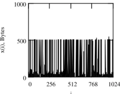
Let x[t(i)] be a series, representing the packet size at time t(i) on a packet-by-packet basis. Then, x(i) stands for a series, indicating the packet size of the ith packet. Traffic series in packet size is of LRD, see e.g. [5-9,23,24,25].
Fig. 4 is the plot of the first 1024 points of x(i) for DEC WRL-4. Fig. 5 is the correlation matrix consisting of 90 sample autocorrelations of x(i). From Fig. 5, one sees that the minimum value of the element in C is greater than 0.912, meaning that rl(k)
of x(i) of DEC WRL-4 does not vary considerably as
l changes. Thus, x(i) of DEC WRL-4 is stationary.
0 256 512 768 1024 0 1000 2000 i x( i), By te s
Fig. 4. Real traffic DEC WRL-4 in packet size. 1
0.912
C
Fig. 5. Correlation matrix consisting of 90 sample autocorrelations of x(i) of DEC WRL-4.
4 Discussions
The research of traffic exhibits that traffic has the property of multifractal either on a point-by-point basis or on an interval-by-interval basis, see e.g. [17-20]. We note that the concept of the stationarity differs from that of multi-fractality. The former implies that r(k; l) does not vary significantly with l
while the latter means that the statistical parameter, such as the Hurst parameter H or fractal dimension D, is time varying. To be precise, time varying H or D of the investigated traffic series may not imply that series is nonstationary unless r(k; l) changes considerably with l.
Note that the meaning of ‘considerably’ or ‘significantly’ is characterized by the correlation threshold. The selection of the correlation threshold γ, however, relies on the individual researchers, usually ranging from 0.7 to 0.9 or greater than 0.9 in engineering. Thus, high value of γ, e.g., γ = 0.95, implies strict classification of stationarity or nonstationarity. Nevertheless, over-high value of γ may be inappropriate when one takes into account measurement errors or computation errors, such as errors in autocorrelation estimation, and or uncertainties. On the other side, low value of γ, e.g., γ = 0.65, may yield rough classification. We use a traffic trace named Lbl-pkt-5 to explain this further. That trace was recorded at the Lawrence Berkeley Laboratory [14]. It contains 710614 packets.
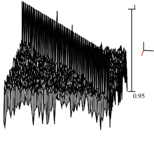
Let x(i) be a series, representing the size of the ith packet of Lbl-pkt-5. Fig. 6 is the plot of x(i). Due to relatively short sample size, we only section x(i) into 10 non-overlapped sections. Thus, the correlation matrix for Lbl-pkt-5 is 10×10, see Fig. 7.
The minimum element of C equals to 0.865. Therefore, x(i) of Lbl-pkt-5 is stationary in the sense of γ = 0.85 but it may be taken as nonstationary if one sets γ > 0.865. 0 256 512 768 1024 0 500 1000 i x( i), By te s
1
0.865
C
Fig. 7. Correlation matrix consisting of 10 sample autocorrelations of x(i) of Lbl-pkt-5.
5 Conclusion
We have discussed a method to do the weak stationarity test of traffic with LRD as a single history series of finite length.
Acknowledgements
This work was supported in part by the National Natural Science Foundation of China under the project grant number 60573125, and by the Shanghai Leading Academic Discipline Project under the project number B411.
References:
[1] A. Papoulis, Probability, Random Variables, and Stochastic Processes, New York, McGraw-Hill, 1984.
[2] G. A. Korn and T. M. Korn, Mathematical Handbook for Scientists and Engineers, McGraw-Hill, 1961.
[3] J. S. Bendat and A. G. Piersol, Random Data: Analysis and Measurement Procedure, 2nd
Edition, John Wiley & Sons, 1991.
[4] D. P. Heyman and T. V. Lakshman, On the Relevance of Long-Range Dependence in Network Traffic, IEEE/ACM Trans. Networking, Vol. 7, No. 5, June. 1999, pp. 629-640.
[5] P. Abry and D. Veitch, Wavelet Analysis of Long-Range Dependent Traffic, IEEE Trans. Information Theory, Vol. 44, No. 1, Jan. 1998, pp. 2-15.
[6] W. Willinger and V. Paxson, Where Mathematics Meets the Internet, Notices of the American Mathematical Society, Vol. 45, No. 8,
Aug. 1998, pp. 961-970.
[7] H. Michiel and K. Laevens, Teletraffic Engineering in a Broad-Band Era, Proc.the
IEEE, Vol. 85, No. 12, Dec., 1997, pp.
2007-2033.
[8] B. Tsybakov and N. D. Georganas, Self-Similar Processes in Communications Networks, IEEE Trans. Information Theory, Vol. 44, No. 5, Sep. 1998, pp. 1713-1725.
[9] V. Paxson and S. Floyd, Wide Area Traffic: the Failure of Poisson Modeling, IEEE/ACM Trans. Networking, Vol. 3, No. 3, June 1995, pp. 226-244.
[10] S. Floyd and V. Paxson, Difficulties in Simulating the Internet, IEEE/ACM Trans. Networking, Vol. 9, No. 4, Aug. 2001, pp. 392-403.
[11] J. Beran, Statistics for Long-Memory Processes, Chapman & Hall, 1994.
[12] K. S. Fu, Editor, Digital Pattern Recognition, Springer, 1976.
[13] M. Li, et al, An On-Line Correction Technique of Random Loading with a Real-Time Signal Processor for a Laboratory Fatigue Test, J. Testing and Evaluation, Vol. 28, No. 5, Sep. 2000, pp. 409-414.
[14] http://www.acm.org/sigcomm/ITA/
[15] J. L. Talmaon, Pattern Recognition of the ECG: a Structured Analysis, Ph.D. Thesis, 1983. [16] W. Willinger, V. Paxson, R. H. Riedi, and M. S.
Taqqu, Long-Range Dependence and Data Network Traffic, in Long-range Dependence: Theory and Applications, P. Doukhan, G. Oppenheim and M. S. Taqqu, eds., Birkhauser, 2002.
[17] M. S. Taqqu, V. Teverovsky, and W. Willinger, Is Network Traffic Self-Similar or Multifractal?
Fractals, Vol. 5, 1997, pp. 63-73.
[18] M. Li, Change Trend of Averaged Hurst Parameter of Traffic under DDOS Flood Attacks, Computers & Security, Vol. 25, No. 3, May 2006, pp. 213-220.
[19] M. Li, S. C. Lim, and Huamin Feng, A Novel Description of Multifractal Phenomenon of Network Traffic Based on Generalized Cauchy Process, Springer LNCS 4489, May 2007, pp. 1-9.
[20] M. Li, S. C. Lim, B.-J. Hu, and Huamin Feng, Towards Describing Multi-Fractality of Traffic Using Local Hurst Function, Springer LNCS 4488, May 2007, pp. 1012-1020.
[21] C. Liu, J. Yang, and J. Yang, A Nonstationary Traffic Train Model for Fine Scale Inference From Coarse Scale Counts, IEEE J. Selected
Areas in Communications, Vol. 21, No. 6, 2003, pp. 895-907.
[22] D. Rincón and S. Sallent, On-Line Segmentation of Non-Stationary Fractal Network Traffic with Wavelet Transforms and Log-Likelihood-Based
Statistics, Springer LNCS 3375, 2005, pp.
110-123.
[23] M. Li, S. C. Lim, and W. Zhao, Long-Range Dependent Network Traffic: A View from Generalized Cauchy Process, in Progress in Applied Mathematical Modeling, edited by F. Yang and et al., Nova Science Publishers, USA, 321-338, to be published in 2008 1st Quarter. [24] M. Li, and et al., Modeling Autocorrelation
Functions of Self-Similar Teletraffic in Communication Networks Based on Optimal Approximation in Hilbert Space, Applied Mathematical Modelling, Vol. 27, No. 3, 2003, pp. 155-168.
[25] M. Li, Modeling Autocorrelation Functions of Long-Range Dependent Teletraffic Series Based on Optimal Approximation in Hilbert Space-a Further Study, Applied Mathematical Modelling, Vol. 31, No. 3, Mar. 2007, pp. 625-631.
[26] M. Li, W. Jia, and W. Zhao, Correlation Form of Timestamp Increment Sequences of Self-Similar Traffic on Ethernet, Electronics Letters, Vol. 36, No. 19, Sep. 2000, pp. 1168-1169.