Simulation of Electron Cloud Effects in the PETRA Positron Storage Ring

(1)

Simulation of Electron Cloud Eﬀects in the

PETRA Positron Storage Ring

R. Wanzenberg

DESY, Notkestr. 85, 22603 Hamburg, Germany

December 10, 2003

DESY M 03-02 December 2003

Abstract

In positron storage rings electrons produced by photoemission, ion-ization and secondary emission accumulate in the vacuum chamber and form an ”electron cloud ” which can reach a high charge den-sity for some beam operation modes. Electron cloud effects have not been observed in the present operation mode of the PETRA II ring used as a preaccelerator for HERA, but with the high perfor-mance goals of the planned synchrotron radiation facility PETRA III a more complete understanding of electron cloud development and its effects on the positron beam are needed to aid in the design. The computer code ECLOUD 2.3 is used to simulate electron cloud effects for different operation modes of PETRA II and PETRA III. An effective transverse single bunch wakefield due to the electron cloud is obtained from a broad band resonator model.

(2)

1 Introduction

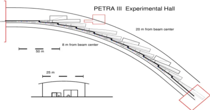
The PETRA ring is presently used as a preaccelerator for the HERA lepton hadron collider ring at DESY. Positron currents of about 50 mA are injected at an energy of 7 GeV and accelerated to the HERA injection energy of 12 GeV. It is planned to rebuild the PETRA ring into a synchrotron radiation facility [1], called PETRA III, after the end of the present HERA collider physics program. One section of the PETRA ring will be completely redesigned to provide space for several undulators. The planned facility aims for a very high brilliance of

about 1021 photons/s/0.1%BW/mm2/mrad2 using a low emittance (1 nm rad)

positron beam with an energy of 6 GeV. The planned location for the new hall is shown in Fig. 1. A more detailed layout of the hall and the synchrotron radiation beam lines is shown in Fig. 2

PETRA

New experimental Hall

Figure 1: Ground plan of the DESY site with the PETRA ring. The location of the planned new experimental hall is also shown.

In positron storage rings electrons produced by photoemission, ionization and secondary emission accumulate in the vacuum chamber forming an ”elec-tron cloud” with a charge density which depends on the beam operation mode. For certain modes with short bunch spacings and high intensities a high cloud density disturbs the beam. Experimental observations of eﬀects due to electron clouds have been reported from existing accelerators operating with high beam current like the B-factories (KEKB, PEP-II) [2, 3]. In 1995, a multi-bunch in-stability, seen at the KEK photon factory since the start of the positron beam operation in 1989, was explained by bunch-to-bunch coupling via electron clouds [5, 4]. Earlier observations of electron clouds, dating back to 1966 and 1977, have been reported from proton storage rings [6, 7]. The present understanding of

(4)

Figure 2: Layout of the new experimental hall for synchrotron radiation experi-ments.

the build-up of an electron cloud and of the eﬀects of the cloud on the positron beam are based on computer simulations and measurements with diﬀerent types of detectors. A summary is given in [8, 9, 10, 11].

Electron cloud effects have not been observed in the present operation mode of the PETRA accelerator as a preaccelerator for HERA (referred to as PETRA II) with moderate bunch currents and relatively large bunch spacings, but with the high performance goals of the planned facility PETRA III a more complete understanding of electron cloud development and its effects on the positron beam are needed to aid in the design. The computer code ECLOUD 2.3 by F. Zimmer-mann et al. [12] is used to simulate electron cloud effects for different operation modes of PETRA II and PETRA III. An example from an electron cloud sim-ulation for PETRA II is shown in Fig. 3. The operation parameters used for the simulations are discussed in the next section while the simulation results are presented in section 3. -0.03 -0.02 -0.01 0 0.01 0.02 0.03 -0.06 -0.04 -0.02 0 0.02 0.04 0.06 y / m x / m

Figure 3: Simulation of an electron cloud in the PETRA II vacuum chamber using ECLOUD 2.3.

(5)

2 PETRA II and PETRA III parameters

For the simulation of the build-up of an electron cloud it is important to know the beam parameters, the vacuum chamber geometry and the secondary electron emission yield of the vacuum chamber material. The data for the PETRA II and the planned PETRA III positron storage rings are summarized in this section.

2.1 Beam parameters and beam optics

2.1.1 Beam parameters

Four sets of beam parameters are considered for the electron cloud simulations: PETRA II with 96 ns and 10 ns bunch spacing and two operation modes of the planned synchrotron facility PETRA III. The parameters are summarized

in Tab. 1. The PETRA II parameters with 96 ns bunch spacing are typical

PETRA II PETRA III

96 ns 10 ns A B Energy /GeV 7 7 6 6 Circumference /m 2304.0 2304.0 2304.0 2304.0 Bending radius /m 191.729 191.729 191.729 191.729 Revolution frequency /kHz 130.1 130.1 130.1 130.1 Bunch Population /1010 5.0 4.1 0.5 24.0 Number of bunches 42 14 1920 40

Total current /mA 44 12 200 200

Bunch separation /m 28.78 3 1.2 57.6 /ns 96 10 4 192 Emittance _x/nm 23 23 1 1 _y/nm 0.3 0.3 0.01 0.01 Tune Q_x 25 25 36 36 Q_y 23 23 31 31 Q_s 0.06 0.06 0.05 0.05 Momentum compaction /10−3 2.52 2.52 1.2 1.2 Beta-functions β_x /m 18 18 15 15 β_y /m 19 19 15 15 Beam sizeσ_x /µm 643 643 122 122 σ_y /µm 75 75 12 12 Bunch length /mm 7 7 12 12

Table 1: Assumed PETRA II and PETRA III parameters. These parameter sets are used in this report for the simulation of the electron cloud build-up.

operation parameters when PETRA is running as a preaccelerator for HERA. The injection energy of PETRA is 7 GeV. The beam is ramped up to an energy

(6)

of 12 GeV and transfered into HERA. This operation mode requires a multi-bunch feedback to damp the transverse multi-bunch oscillations. The presently installed feedback system requires a bunch spacing of at least 96 ns due to bandwidth limitations. During machine studies it has been demonstrated that it is possible to operate PETRA with a bunch spacing of only 10 ns but with only 14 bunches without any feedback. The beam marker and bunch signals are shown in Fig. 4 (measured on Feb. 2, 2003). This ﬁll-pattern of PETRA has also been used for some electron cloud simulations to investigate the dependence of the electron cloud density on the bunch to bunch spacing. For PETRA III two parameter sets

Figure 4: Beam marker and bunch signals at PETRA II. Fourteen bunches with a spacing of only 10 ns are ﬁlled in the PETRA ring.

are considered (labeled A and B ) with the same total current but with diﬀerent number of bunches and bunch spacings. It is planned to operate PETRA III predominantly in mode A. The short bunch spacing in mode A of only 4 ns is a concern with respect to the build-up of electron clouds.

2.1.2 PETRA III beam optics

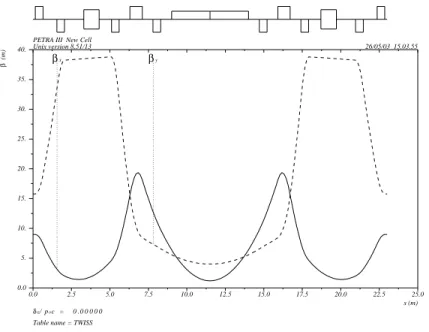
The horizontal and vertical beta-function of a standard PETRA III arc cell and a DBA (double bend achromat) cell of the new ring section [13] are shown in Fig. 5 and Fig. 6. The standard arc cell is a simple FODO cell with a phase

advance of 72◦. The bending radius ρ_B of the 5.378 m long dipole magnet is

ρ_B = 191.729 m. This arc cell is identical to the presently used cell of the

(7)

planned DBA-cell is only 1 m long (bending radius ρ = 22.918 m) to provide suﬃcient space for the installation of an undulator magnet.

0.0 2. 4. 6. 8. 10. 12. 14. 16. s (m)

δE/ p0c = 0 . 0 0 0 0 0 Table name = TWISS PETRA III 72/72 Unix version 8.51/13 27/05/03 08.34.57 6. 8. 10. 12. 14. 16. 18. 20. 22. 24. β (m ) βx βy

Figure 5: Optics of the standard PETRA III arc cell. The horizontal and vertical beta-functions are plotted versus the position.

0.0 2.5 5.0 7.5 10.0 12.5 15.0 17.5 20.0 22.5 25.0 s (m)

δE/ p0c = 0 .0 0 0 0 0

Table name = TWISS PETRA III New Cell

Unix version 8.51/13 26/05/03 15.03.55 0.0 5. 10. 15. 20. 25. 30. 35. 40. β (m ) βx βy

(8)

2.2 The vacuum chamber

The geometry of the vacuum chamber in the PETRA II arc is shown in Fig. 7. The chamber has a octagonal shape which may be approximated with ellipses as shown in Fig. 8. The semi axes of the inner (dotted line) ellipse have the same dimensions of half of the actual chamber width and height, while the vertical semi axis of the outer (solid line) ellipse is 35 mm, which is 7 mm larger than the actual chamber half height. For the computer simulations with the ECLOUD2.3 code a chamber boundary is used which is a combination of a straight line and a short arc of the outer ellipse. The boundary is shown in Fig. 9. The vacuum chamber of the synchrotron light source PETRA III is still in the design phase. One possible layout of the chamber in the arc is shown in Fig. 10. The beam chamber has an elliptical shape with semi axes of 20 mm vertically and 40 mm horizontally. An ante-chamber is housing the integrated vacuum pumps. For the simulations of the electron cloud eﬀects only the central chamber is considered. All chamber dimensions are summarized in Tab. 2. Additionally several charge

PETRA II PETRA III

96 ns 10 ns A B

horizontal semi axis /mm 57 40

vertical semi axis /mm 28 20

chamber area /cm2 55.8 25.1

Bunch Population N₀ /1010 5.0 4.1 0.5 24.0

Bunch separation d/m 28.78 3 1.2 57.6

/ns 96 10 4 192

average bunch charge densities:

volume ρ_b / (1012 m−3) 0.31 2.47 1.66 1.66

line N₀/d/ (1010 m−1) 0.17 1.37 0.42 0.42

Beam size σ_x /µm 643 643 122 122

σ_y /µm 75 75 12 12

Bunch length σ_z /mm 7 7 12 12

Bunch line charge density λ_b/(1012 m−1) 2.85 2.33 0.166 7.98

Neutrality

line charge density λ_n/( 105 m−1) 0.96 7.53 0.156 0.156

Table 2: Vaccum chamber dimensions and beam charge densities of PETRA II and PETRA III.

densities are listed in Tab. 2 which give ﬁrst estimates for the expected electron cloud density if one assumes that regardless of the details of the cloud build-up the electron cloud will ﬁnally neutralise the average (positron) beam charge density. First the average beam charge volume density is calculated:

ρ_b= N0

(9)

where N₀ is the bunch population, A is the area of the vacuum chamber cross

section andd the bunch to bunch distance. For an elliptical chamber the areaA

is simplyπ a b with the vertical and horizontal semi axesa andb of the chamber.

The average bunch line charge density isN₀/d, while the bunch line charge density

λ_b is

λ_b = √N0

2π σ_z.

The neutrality line charge density is deﬁned as:

λ_n= 2π σ_xσ_y ρ_b,

whereσ_x and σ_y are the horizontal and vertical rms beam sizes. This densityλ_n

is a ﬁrst approximation for the electron cloud density within the beam, based on the assumption that the average volume charge density of the electron cloud and the positron beam is ﬁnally equal to zero (neutralization condition).

(10)

-40 -30 -20 -10 0 10 20 30 40 -60 -50 -40 -30 -20 -10 0 10 20 30 40 50 60 y / mm x / mm

Figure 8: Approximation of the PETRA II chamber with ellipses.

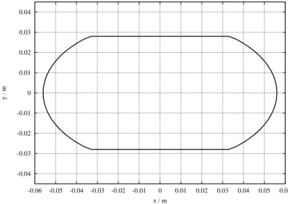
-0.04 -0.03 -0.02 -0.01 0 0.01 0.02 0.03 0.04 -0.06 -0.05 -0.04 -0.03 -0.02 -0.01 0 0.01 0.02 0.03 0.04 0.05 0.06 y / m x / m

Figure 9: Boundary of the PETRA II chamber used for simulations with the ECLOUD code.

(11)

Figure 10: One possible design of the vacuum chamber of the planned PETRA III ring.

2.3 Photoelectrons and secondary emission

2.3.1 Photoelectrons

A relativistic electron or positron which is bent by a magnetic ﬁeld will radiate electromagnetic ﬁelds or in a quantum view will emit photons. The mean number of photons emitted per length is given as:

dN_γ dz = 5 2√3αf E m₀c2 1 ρ, (1)

where E is the energy of the positron beam, m₀ the rest mass of the electron,

ρ the bending radius of the dipole magnet and α_f = e2/(4π ₀h c¯ ) ≈ 1/137.

Photoelectrons are emitted from the chamber walls at a rate of

dN_e−

dz =Yeff

dN_γ

dz , (2)

where Y_eff is the eﬀective photoelectron emission yield. The total number of

photoelectrons per length generated from one bunch is N₀dN_e−/dz, where N₀

is the bunch population. The eﬀective photoelectron emission yield depends on the photon spectrum, the photoelectric yield of the material and on the photon reﬂectivity of the chamber.

The photoelectric yield of Aluminum as a function of the photon energyη_pe(u) shown in Fig. 11 for normal incidence is obtained from reference [14], which is based on the results of measurements.

The power spectrum of the photons is given by [15, 16]: P(ω) = Pγ

(12)

0.0001 0.001 0.01 0.1 1 1 10 100 1000 10000 100000 1e+06 Photoelectric yield Photon energy / eV

Figure 11: Photoelectric yield of Aluminum for normal incidence. where the functionS(x) is deﬁned as

S(x) = 9 √ 3 8π x _∞ x dζ K53(ζ), (4)

using the Bessel function of the third kind of order 5/3. Furthermore, ω_c =

(3/2) (c/ρ)γ3 is the critical frequency of the photons, and P_γ = ₀∞dωP(ω) the total power.

The photon density n(u) as a function of the photon energy u is obtained

from the power spectrum:

n(u) = 1

u

1 ¯

hP(u/¯h), (5)

which can be rewritten as

n(u) = Pγ

u_c2F(u/uc), (6)

where F(x) = S(x)/x and u_c = ¯h ω_c is the critical energy of the photons. The

power spectrum S(u/u_c) and the photon density F(u/u_c) are show in Fig. 12.

(One obtains for the integrals: ₀∞dsS(x) = 1 and ₀∞dsF(x) = 15√3/8.)

The eﬀective photoelectron emission yield for normal incidence Y_⊥ can be

calculated as: Y_⊥ = _∞ 0 du ηpe(u)n(u) ∞ 0 du n(u) , = 8 15√3 _∞ 0 du u_c ηpe(u)F(u/uc). (7)

(13)

0 0.2 0.4 0.6 0.8 1 0 1 2 3 4 5 Photon density

Photon energy / critical photon energy

Power density Photon density

Figure 12: Number of photons per energy and photon power spectrum. A plot of photoelectron yield times the photon densityF(u/u_c) is shown in Fig. 13

for a critical energy of about 2.5 keV corresponding to a beam energy of 6 GeV

and a bending radius of about 192 m. For these parameters one obtains an

eﬀective photoelectron emission yield of about 0.05 for normal incidence photons

(see Tab. 3). 0 1 2 3 4 5 6 7 8 9 10 1 10 100 1000 10000

Photoelectric yield * photon density

Photon energy / eV

Yield * F(u)

Figure 13: The product of the photoelectric yield of Aluminum and the photon density for a beam energy of 6 GeV.

The effective photoelectron yield for photons at grazing incidence can either be significantly enhanced or reduced, depending on the reflection coefficient of

(14)

PETRA II PETRA III

Energy /GeV 7 6

Bending radius ρ/m 191.729 191.729

u_c /keV 3.968 2.499

Y_⊥ 0.047 0.042

Table 3: Eﬀective photoelectron yield for normal incidence.

the photons [14, 17, 18] which is difficult to know precisely. The number of photoelectrons in the vacuum chamber will be reduced for chamber designs with an ante-chamber. As a result of these unknown factors the precise value for the effective photoelectron yield is not know. For most of the simulations an effective photoelectron yield of

Y_eff ≈0.1 (8)

will be used, which is about a factor of two larger than that calculated for nor-mal incidence photons assuming that no ante-chamber is present. An eﬀective

photoelectron yield of 0.1 is reported also for the KEK B-factory [19] vacuum

chamber. For some of the simulations an even higher photoelectron yield of

Y_eff = 1 is used to examine the dependence of the electron cloud density on the

number of primary generated photoelectrons. The photoelectron emission rates are summarized for PETRA II and PETRA III in Tab. 4.

PETRA II PETRA III

96 ns 10 ns A B Energy /GeV 7 7 6 6 Bunch Population N₀/1010 5.0 4.1 0.5 24.0 Bending radius ρ/m 191.729 191.729 191.729 191.729 dN_γ/dz / m 0.753 0.753 0.645 0.645 Y_eff 0.1 0.1 0.1 0.1 dN_e−/dz / m 0.075 0.075 0.065 0.065 N₀dN_e−/dz /( 1010 m) 0.376 0.309 0.032 1.549

Table 4: Photoelectron emission rates for PETRA II and PETRA III.

2.3.2 Secondary emission

The mean energy of the (primary) photoelectrons is about 7 eV. The electric ﬁeld of the trailing bunches will accelerate the photoelectrons up to several hundred eV depending on the bunch population and the chamber dimensions. A photo-electron which hits the vacuum chamber wall can generate secondary photo-electrons

with a secondary emission yield δ_SE(E) which depends on the energy of the

pri-mary electron and on the material properties. The following data enter into the simulation recipe of the ECLOUD 2.3 code [12].

(15)

The measured data [20] for the secondary emission yield can be described analytically, as suggested by M. Furman [21], in the following way:

δ_SE(E) =δ_max s (E/Emax)

s−1 + (E/E_max)s, (9)

with three material dependent parametersδ_max,E_max ands, which depend on the

angle of incidence of the primary electron with respect to the material surface. The secondary emission yield of a non pure (technical) material depends strongly on the surface properties of the material. Various surface treatments have been investigated [22] to reduce the secondary emission yield. A very powerful method to circumvent the problems due to electron multiplication is the ”dose eﬀect” (or processing). Typical parameters for copper and aluminum after processing are given in Tab. 5. Copper ”as received” may have a secondary emission parameter

δ_max of more than 2.0 and aluminum ”as received” of more than 3.0. With a

Cu Al

δ_max 1.4 2.2

E_max / eV 240 300

s 1.39 1.35

Table 5: Parameters for the secondary emission yield for copper and aluminum (normal incidence).

certain probability the primary electrons which hit the surface interact in an inelastic way with the material yielding ”true secondary” electrons. But some electrons are elastically backscattered oﬀ the surface. The Eqn. (9) refers to the true secondary electron yield which is plotted in Fig. 14 as solid curves for copper and aluminum using the parameters from Tab. 5. The total secondary emission yield can be written as a sum of the true secondary electron yield and the reﬂected electron yield:

δ_tot(E) = δ_SE(E) +δ_R(E) =δ_SE(E) 1

1−f_R(E), (10)

where the factorf_R(E) gives the yield from reflected electrons as a fraction of the total yield (δ_tot =f_R δ_SE). The fraction of reflected electrons has been measured as a function of the primary energy. A fit to the data gives for primary energies below 300 eV [20]:

f_R(E) = expA₀+A₁ ln(B+E/eV) +A₂(ln(B+E/eV))2, (11) with A₀ = 20.7, A₁ = −7.08, A₂ = 0.484 and B = 56.9. The total secondary emission yield is plotted in Fig. 14 as dashed curves for copper and aluminum. The reﬂected component contributes signiﬁcantly to the total secondary electron

(16)

yield for primary electron energies of a few eV. Besides the true secondary and reflected electrons there is a third component to the total secondary electron yield, which is refered to as ”rediffused” electrons. These are electrons which penetrate into the material and undergo multiple scattering inside the material before being reflected back out the material. This component is neglected in simulations with ECLOUD 2.3. The energy distribution of the true secondary

0 0.5 1 1.5 2 2.5 0 100 200 300 400 500 600 700 800 900 1000 SEY E / eV

Cu, true secondaries Cu Al, true secondaries Al

Figure 14: Secondary emission yield for copper and aluminum vacuum cham-bers. The contribution from the reﬂected electrons is included in the total yield presented with the dashed curves.

electrons is ﬁtted with the following formula [23]:

D(E) = C exp −(ln(E/E0))2 2τ2 , (12)

where C, τ and E₀ are parameters to ﬁt the measured data. The energy

dis-tribution is plotted in Fig. 15 for C = 0.2, τ = 1 and E₀ = 1.8 eV. The slight

dependence of the parameters on the energy of the primary electron is neglected

(17)

0 0.02 0.04 0.06 0.08 0.1 0.12 0.14 0.16 0.18 0.2 0 1 2 3 4 5 6 7 8 Energie distribution E / eV

(18)

3 Simulation of the electron cloud build-up

For all electron cloud simulations the code ECLOUD 2.3 has been used [12]. The beam parameters and the vacuum chamber dimensions have been taken from Tab. 1 and Tab. 2. If not stated otherwise the photoelectron emission rates are

based on an eﬀective photoelectron yield of 0.1 (see Tab. 4). The parameters for

the secondary emission yield for a aluminum chamber with maximum yield δ_max

of 2.2 have been assumed (see Tab. 5) for PETRA II and PETRA III. Plots of

the electron cloud population and the electron cloud density in the bunch center are presented in the following subsections. The results are summarized in a table at the end of this section.

3.1 PETRA II

3.1.1 PETRA II – Standard ﬁll with 96 ns bunch spacing

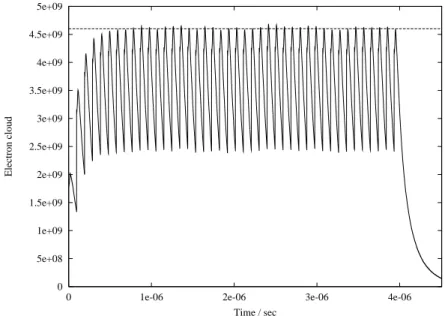
In the PETRA II storage no performance degradations due to electron clouds have been observed during the standard operation mode with a bunch spacing of 96 ns. The simulation (using the ECLOUD 2.3 code) predicts an electron

cloud build-up during about 5×95 ns to a total cloud population of 0.46·1010

electrons per meter as shown in Fig. 16. This corresponds to an average cloud density of 0.83·1012 m−3. The electron cloud center density, as obtained from

0 5e+08 1e+09 1.5e+09 2e+09 2.5e+09 3e+09 3.5e+09 4e+09 4.5e+09 5e+09

0 1e-06 2e-06 3e-06 4e-06

Electron cloud

Time / sec

Figure 16: Simulated population of the electron cloud build-up in the PETRA II vacuum chamber using ECLOUD 2.3. The dashed line indicates a population of 0.46·1010/m.

(19)

Fig. 18. Although there are ﬂuctuations the electron center density is found to be about 0.7·1012 m−3 as indicated in Fig. 18.

0 2e+11 4e+11 6e+11 8e+11 1e+12

0 1e-06 2e-06 3e-06 4e-06

Electron cloud volume density / m-3

Time / sec

Figure 17: Electron cloud center density in the PETRA II vacuum chamber (results from ECLOUD 2.3).

0 2e+11 4e+11 6e+11 8e+11 1e+12

1e-06 1.5e-06 2e-06

ecloud volume density / m-3

time

Figure 18: Detail of electron cloud center density in the PETRA II vacuum chamber (results from ECLOUD 2.3). The cloud population is also shown for reference, plotted in arbitrary units (dashed line). The dashed line indicates a density of 0.7 1012m−3.

(20)

3.1.2 PETRA II – Special ﬁll with 10 ns bunch spacing

During machine studies PETRA II was operated with a special ﬁll pattern with a bunch spacing of only 10 ns. The simulation of the electron cloud population in this case is shown in Fig. 19. At the end of the bunch train a population of

1.4·1010 electrons per meter is reached, corresponding to an average electron

cloud density of 2.5·1012 m−3, which is about a factor of 3.5 higher than in the standard ﬁll pattern with 96 ns bunch spacing. The equilibrium electron cloud population is not reached within the short bunch train of only 14 bunches. A short gap is suﬃcient to let the cloud population decay by a factor of two. The

0 2e+09 4e+09 6e+09 8e+09 1e+10 1.2e+10 1.4e+10 1.6e+10

0 5e-08 1e-07 1.5e-07

Electron cloud

Time / sec

Figure 19: Simulated population of an electron cloud in the PETRA II (10 ns) vacuum chamber using ECLOUD 2.3.

simulation result for the electron cloud center density is shown in Fig. 20. As indicated by the dashed line in the figure a center density of about 2.1·1012m−3is reached at the end of the bunch train. The center density and the average density do not differ significantly and are similar to the neutrality density of 2.4·1012m−3 (see Tab. 2).

(21)

0 5e+11 1e+12 1.5e+12 2e+12 2.5e+12 3e+12

0 5e-08 1e-07 1.5e-07

Time / sec

Figure 20: Electron cloud center density in the PETRA II (10 ns) vacuum cham-ber using ECLOUD 2.3. The dashed line indicates a density of 2.1 1012m−3.

3.2 PETRA III

The two parameter sets for PETRA III (labeled A and B, see Tab. 1) have been considered for the simulations with the ECLOUD 2.3 code. Fig. 21 shows the distribution of the macro particles in the elliptical vacuum chamber at diﬀerent time steps during the simulation. The electron cloud population, average and center cloud densities are presented in the following subsections.

-0.02 -0.01 0 0.01 0.02 -0.05 -0.04 -0.03 -0.02 -0.01 0 0.01 0.02 0.03 0.04 0.05 y / m x / m -0.02 -0.01 0 0.01 0.02 -0.05 -0.04 -0.03 -0.02 -0.01 0 0.01 0.02 0.03 0.04 0.05 y / m x / m

Figure 21: Simulation of an electron cloud build-up in the PETRA III vacuum chamber using ECLOUD 2.3. The macro particle distributions at two diﬀerent times are shown in the two graphs.

(22)

3.2.1 PETRA III – Variant A

First the parameter set A with many bunches and a small bunch spacing of only 4 ns is considered. The build-up of the electron cloud population simulated with the ECLOUD 2.3 code is shown in Fig. 22. A equilibrium population of about 3.2·1010is reached after about 100 bunches of the bunch train. This corresponds

to an average electron cloud population of 1.3·1012 m−3. The corresponding

0 5e+08 1e+09 1.5e+09 2e+09 2.5e+09 3e+09 3.5e+09

0 1e-07 2e-07 3e-07 4e-07

Electron cloud

Time / sec

Figure 22: Simulation of the electron cloud population in the PETRA III-A vacuum chamber using ECLOUD 2.3. The dashed line indicates an electron cloud population of 0.32·1010.

results for the electron cloud center density are show in Fig. 23 and in detail for a shorter time interval in Fig. 24. The center density of about 1.0·1012 m−3 is almost equal to the average electron cloud density.

(23)

0 2e+11 4e+11 6e+11 8e+11 1e+12 1.2e+12 1.4e+12

0 1e-07 2e-07 3e-07 4e-07

Time / sec

Figure 23: Simulation of the electron cloud center density in the PETRA III-A vacuum chamber using ECLOUD 2.3.

0 2e+11 4e+11 6e+11 8e+11 1e+12 1.2e+12 1.4e+12

3e-07 3.25e-07 3.5e-07

Time / sec

Figure 24: Detail of the electron cloud center density in the PETRA III-A vacuum chamber using ECLOUD 2.3.

(24)

Simulations with a eﬀective photoelectron yield of 1.0.

An eﬀective photoelectron yield of 0.1 has been normally assumed for the

simu-lations. To study the dependence of the electron cloud density on this parameter the previous simulations of PETRA III (variant A) has been repeated with a

photoelectron yield of 1.0 and with otherwise unchanged parameters. The results

for the bunch population are shown in Fig. 25. The electron cloud population is 1.5·1010per meter for this case, which is a factor of 4.7 higher compared with the previous simulation with a ten times lower photoelectron yield. The

correspond-0 2e+09 4e+09 6e+09 8e+09 1e+10 1.2e+10 1.4e+10 1.6e+10

0 1e-07 2e-07 3e-07 4e-07

Electron cloud

Time / sec

Figure 25: Simulation of the electron cloud population in the PETRA III-A vacuum chamber using ECLOUD 2.3. The line indicates an electron cloud pop-ulation of 1.5·1010. A photoelectron yield of 1.0 has been assumed.

ing center density of the electron cloud is shown in Fig. 26. The line indicates a center density of 3.5·1012 m−3 which is a factor 3.5 higher than in the case with a photoelectron yield of 0.1.

(25)

0 1e+12 2e+12 3e+12 4e+12 5e+12 6e+12

0 1e-07 2e-07 3e-07 4e-07

Time / sec

Figure 26: Simulation of the electron cloud center density in the PETRA

III-A vacuum chamber using ECLOUD 2.3. III-A photoelectron yield of 1.0 has been

assumed.

3.2.2 PETRA III – Variant B

No electron cloud build-up over the bunch train is found in the simulation results for a large bunch spacing of 192 ns (parameter set B). Each bunch induces an electron cloud with a population of about 2.2·1010 which decays before the next bunch of the train arrives. This corresponds to an average electron density of 8.7·1012m−3. A center density of about 1.5·1012m−3is found from the simulations (see Fig. 28).

3.2.3 Summary of the PETRA simulation results

The previously discussed results are summarized in Tab. 6 for the reference pa-rameter set with an photoelectron yield of 0.1. The average electron cloud density has been calculated from the electron cloud population and the vacuum chamber dimensions.

One simulation for PETRA III (variant A) has been done with an photoelec-tron yield of 1.0. For that case a cloud population of 1.5·1010, corresponding to an average cloud density of 5.96·1012m−3, was obtained. The center density was 3.5·1012 m−3.

(26)

0 5e+09 1e+10 1.5e+10 2e+10 2.5e+10

0 1e-06 2e-06 3e-06 4e-06 5e-06 6e-06 7e-06 8e-06 9e-06

e-cloud

Time

Figure 27: Simulation of the electron cloud population in the PETRA III-B vacuum chamber using ECLOUD 2.3.

0 5e+11 1e+12 1.5e+12 2e+12 2.5e+12 3e+12 3.5e+12 4e+12 4.5e+12 5e+12

0 1e-06 2e-06 3e-06 4e-06 5e-06 6e-06 7e-06 8e-06 9e-06

ecloud volume density / m-3

time

Figure 28: Simulation of the electron cloud center density in the PETRA III-B vacuum chamber using ECLOUD 2.3.

(27)

PETRA II PETRA III

96 ns 10 ns A B

chamber area /cm2 55.8 25.1

Bunch Population N₀ /1010 5.0 4.1 0.5 24.0

Bunch separation /ns 96 10 4 192

volume ρ_b / (1012 m−3) 0.31 2.47 1.66 1.66

Results from the simulations

Cloud Population /1010/ m 0.46 1.4 0.32 2.2

Average density /(1012 m−3) 0.83 2.5 1.3 8.7

Center density / (1012 m−3) 0.7 2.1 1.0 1.5

(28)

3.3 KEK-B LER

A vertical emittance growth due to an instability caused by electron clouds has been observed in the low energy ring (LER) of the KEK B-Factory for beam intensities above 500 mA in the case that no solenoids are switched on as a coun-termeasure [2, Fig. 16]. The code ECLOUD 2.3 has also been used to simulate the build-up of the electron cloud in the KEKB LER using the parameters from Tab.7 and 8, which have been compiled from [24, 2].

KEK-B LER Energy /GeV 3.5 Circumference /m 3016 Bending radius /m 15.9 revolution frequency /kHz 99.4 Bunch Population /1010 3.0 Number of bunches 1200

Total current /mA 573

Bunch separation /m 2.39 /ns 8 Emittance _x/nm 18 _y/nm 0.0036 Tune Q_x /Q_y 46 / 46 Q_s 0.01 Momentum compaction /10−4 ∼1 Beta-functions β_x/β_ey /m / 15 / 15 Beam sizeσ_x / σ_y /µm 520 / 7 Bunch length /mm 4

Table 7: Assumed KEK B LER parameters (part 1). These parameter sets are used for the simulation of the electron cloud build-up in the KEK B-factory low energy ring.

A secondary emission yield of 1.4 (see Tab.5) has been assumed for the copper

chamber. A ﬁeld free region has been considered for the simulations. The results of the simulation of the electron cloud population are shown in Fig. 29. An equi-librium population of 2.9·1010electrons per meter is obtained. This corresponds to an average electron cloud density of 4.2·1012 m−3. The electron cloud center density obtained from the simulation with ECLOUD 2.3 is shown in Fig. 30. The center density of the cloud is about 3.0·1012 m−3. This is about a factor of three larger than the simulated center density for PETRA III variant A.

(29)

KEK-B LER Vacuum chamber

chamber radius /mm 47

chamber area /cm2 69.3

volume ρ_b / (1012 m−3) 1.8

line N₀/d/ (1010 m−1) 2.91

Bunch line charge density λ_b/(1012 m−1) 2.99

Neutrality

line charge density λ_n/( 105 m−1) 0.43

Photoelectron emission rates

dN_γ/dz / m 4.538

Y_eff 0.1

dN_e−/dz / m 0.4538

N₀dN_e−/dz /( 1010 m) 1.362

Table 8: Assumed KEK B LER parameters (part 2). These parameters are used for the simulation of the electron cloud build-up in the KEK B-factory low energy ring. 0 5e+09 1e+10 1.5e+10 2e+10 2.5e+10 3e+10 3.5e+10 4e+10

0 1e-07 2e-07 3e-07 4e-07 5e-07 6e-07 7e-07

Electron cloud

Time / sec

Figure 29: Simulated population of the electron cloud in the KEK-B vacuum

(30)

0 5e+11 1e+12 1.5e+12 2e+12 2.5e+12 3e+12 3.5e+12 4e+12 4.5e+12 5e+12

0 1e-07 2e-07 3e-07 4e-07 5e-07 6e-07 7e-07

Time / sec

Figure 30: Electron cloud center density in the KEK-B vacuum chamber (results from ECLOUD 2.3).

(31)

4 Single bunch instabilities due to electron clouds

4.1 Broad band resonator model

A broad band resonator model has been developed in [25, 26] to characterize the interaction between the positron bunch and the electron cloud. The basic

ingredients of the model are the line charge densities λ_b and λ_c of the positron

beam and of the electron cloud, and the transverse beam sizes (σ_x and σ_y). It

is assumed that the electron cloud has the same transversal dimensions as the beam. The line charge density of the cloud is therefore λ_c = 2π σ_xσ_y ρ_c, where

ρ_c is the volume charge density in the center of the vacuum chamber obtained

from computer simulations. The dipole wake can be written as:

w₁(s) = ˆw₁ sin ω_c s c exp −ωc 2Q s c , (13) with ˆ w₁ = γ r_ec3 1 λ_b ω 2 b ωcC, (14) and ω_b2 = 1 γ r_ec2 (σ_x+σ_y)σ_y λc, ω 2 c = r_ec2 (σ_x+σ_y)σ_y λb, (15)

withr_e the classical electron radius,γ the beam energy measured in units of the

rest mass, and C the circumference of the ring. The dipole wake within a bunch

can be calculated as the convolution integral of the point charge wakew₁(s) with the Gaussian charge density in the bunch g(s) = exp(−1₂(s/σ_z)2)/(σ_z√2π):

W₁(s) =

_∞

0 dξ g(s−ξ) w1(ξ). (16)

The ”cloud” frequency ω_c is the frequency of the broad band resonator. This

frequency depends only on the properties of the positron beam. All parameters of the broad band resonator which do not depend directly on the cloud population are summarized in Tab. 9. A Q-value of 5 has been assumed to take into account the broad band characteristic of the impedance.

The normalized point charge wake potential w₁(s)/wˆ₁ as well as the bunch wake potentialW₁(s)/wˆ₁ are shown in Fig. 31 for the PETRA III-A parameters. The dash-dotted line in Fig. 31 shows the charge distribution of the bunch. The eﬀect of the wakeﬁeld due to the electron cloud is greatly reduced since the wavelength (2π c)/ω_c of the point charge wakepotential is smaller than the bunch length. The quantity W₁(σ_z)/wˆ₁ is the bunch wake potential at the position

s = σ_z (tail of the bunch) normalized to the amplitude ˆw₁ of the point charge

wake potential (see Tab. 9). In a two particle model the quantity W₁(σ_z) is used as an estimate of the wake from the head particle acting on the tail particle.

(32)

PETRA II PETRA III KEK-B LER 96 ns 10 ns A B 573 mA Bunch Population /1010 5.0 4.1 0.5 24.0 3.0 cloud frequency ω_c / (2π GHz) 18.35 16.61 25.42 176.13 70.40 W₁(σ_z)/wˆ₁ 0.108 0.134 0.039 0.005 0.042 Q-value ∼5 ∼ 5 ∼ 5

Table 9: Parameters for the broad band resonator model which depend only on the positron beam properties.

-0.8 -0.6 -0.4 -0.2 0 0.2 0.4 0.6 0.8 1 -4 -3 -2 -1 0 1 2 3 4 5

Normalized Wake potential

position

bunch point charge wake bunch wake

Figure 31: Normalized wake potential of electron clouds in PETRA III (parameter set A). The position within the bunch is measured in units of the rms bunch length

σ_z.

4.2 Estimates for the instability thresholds

The strong-head tail instability can be treated in a simpliﬁed way using a two particle model [27]. The equations of motion during the time 0 < s/c < T_s/2, whereT_s= 1/f_s is the synchrotron oscillation period, are

d2 ds2 y1+ ω_β(δ₁) c ₂ , y₁ = 0 (17) d2 ds2 y2+ ω_β(δ₂) c ₂ y₂ = 1 m_ec2γe q 1 CW⊥y1,

wherey₁ and y₂ are the transverse coordinates of macroparticles 1 and 2,δ₁ and

δ₂ are the relative energy deviations (∆E/E) of macroparticles from the design

(33)

W⊥ the eﬀective dipole wake. During the time period Ts/2 < s/c < Ts the

equations of motion are again Eqn. (17) but with indices 1 and 2 exchanged. For the time interval T_s < s/c < 3T_s/2 Eqn. (17) applies again, and so forth. The eﬀective wake due to the head macroparticle can be estimated as the wake within the bunch ats =σ_z:

W⊥ =W1(σz). (18)

The solution of the equations of motion (17) for zero chromaticity are:

y_n(s) =y_n(s) exp(−iΦ_βn(s)), n = 1,2 (19)

where Φ_βn(s) is the betatron phase and the amplitude functions y_n(s) are solu-tions of the equation [27]:

y₁ y₂ s=c Ts = 1−Υ2 iΥ iΥ 1 y₁ y₂ s=0 , (20)

with the parameter Υ, given by

Υ = 1 m_ec2γe 2_N 1 CW⊥ π 2 c2 ω_β ω_s. (21)

The transverse motion is stable if the trace of the matrix in Eqn. (20) is smaller than 2 or equivalently if

Υ<2. (22)

Equations (21) and (22) are used to obtain an upper limit for the eﬀective wake

W⊥ for the considered parameter sets. The results are summarized in Tab. 10.

PETRA II PETRA III KEK-B LER

96 ns 10 ns A B 573 mA Energy /GeV 7 7 6 6 3.5 Circumference /m 2304 2304 2304 2304 3016 N /1010 5.0 4.1 0.5 24.0 3.0 Q_y 23 23 31 31 43 Q_s 0.06 0.06 0.05 0.05 0.01 W⊥limit / (MV/(nC m)) 26.3 32.1 253.6 5.3 5.5 (NW_⊥)_limit / (1010 MV/(nC m)) 131.5 131.5 126.6 126.6 16.3 Table 10: Limit for the wakeﬁeld

The PETRA III (variant A) design is by a factor of about 50 less sensitive to head-tail instabilities than the considered KEK-B LER variant with a bunch

(34)

the considered KEK-B LER variant are almost the same. It is also interesting to translate the condition from Eqn. (22) into a limit on the product of the bunch

population and the eﬀective wakeﬁeld (NW_⊥). The results are shown in the last

row of Tab. 10. It turns out that the KEK-B LER is by a factor of about 8 more sensitive to head-tail instabilities than the PETRA II/III rings which do not diﬀer signiﬁcantly with respect of this parameter (NW_⊥)_limit.

4.3 Wakeﬁelds due to electron clouds

The wakeﬁeld of the electron cloud can be calculated from the electron cloud density according to Eqn. (14) and (16). The results are presented in Tab. 11, ﬁrst under the assumption that the cloud density is equal to the average beam density (neutrality condition) and using the results for the center density from the

computer simulations with the ECLOUD 2.3 code. The transverse wakeﬁelds

PETRA II PETRA III KEK-B LER

96 ns 10 ns A B 573 mA

Condition of neutrality

volume density ρ_b / (1012 m−3) 0.31 2.47 1.66 1.66 1.8

line charge density λ_n/( 105 m−1) 0.96 7.53 0.156 0.156 0.43

ω_bn/(2π) / kHz 28.7 80.6 71.9 71.9 102.3 ˆ w₁_n / (MV/(nC m) 4.9 42.8 628.9 90.7 149.2 W₁(σ_z)_n / (MV/(nC m) 0.53 5.7 24.3 0.49 6.27 W₁(σ_z)_n/W_⊥_limit 0.02 0.18 0.096 0.093 1.15 Simulation center density / (1012 m−3) 0.7 2.1 1.0 1.5 3.0

line charge density λ_c/( 105 m−1) 2.14 6.41 0.094 0.141 0.72

ω_b/(2π) / kHz 42.9 74.3 55.8 68.4 131.9

ˆ

w₁ /(MV/(nC m) 11.0 36.5 379.1 82.1 248.4

W₁(σ_z) /(MV/(nC m) 1.2 4.9 14.7 0.45 10.4

W₁(σ_z)/W_⊥_limit 0.045 0.15 0.058 0.085 1.91 Table 11: Eﬀective transverse wakeﬁeld due to the electron cloud. The results are based on estimates from the condition of neutrality and on the center density

obtained from computer simulations. W₁(σ_z) is the dipole wakepotential at the

position s=σ_z in the tail of the bunch.

W₁(σ_z) due to the electron cloud have been compared with the previously

calcu-lated limit from the instability threshold. The wakeﬁeld is well below (<0.2) the instability threshold for all considered parameter sets for PETRA II/III. For the considered KEK-B LER parameters a head-tail instability is expected since the wakeﬁeld due to the electron cloud is above the limit. This is in agreement with the experimental observations of a beam blow-up [2]. The condition of neutrality seems to be in most cases a very useful estimate of the electron cloud density.

(35)

The results of the simulation PETRA III with a photoelectron yield ofY = 1.0 is not included in Tab. 11. The center density for that case is 3.5·1012m−3, from

which an eﬀective transverse wake of W₁(σ_z) = 51.4 MV/(nC m) is obtained.

This is still well below the instability threshold (W₁(σ_z)/W_⊥_limit = 0.2 ).

5 Summary and conclusion

It is planned to rebuild the PETRA ring, presently used as a preaccelerator for the HERA rings, into a third generation synchrotron light source, called PETRA III. Since it is considered to use a positron beam for PETRA III the build-up of electron clouds was investigated and presented in this paper. In section 2 the parameters of the present PETRA ring and the planned PETRA III storage ring needed for simulations, namely beam and optics parameters as well as the vacuum chamber dimensions, have been introduced. The production of photoelectrons has been estimated from the material properties of Aluminum. The parameters which are important for the production of secondary electrons have been discussed, too. The computer code ECLOUD 2.3 has been used to simulate the electron cloud build-up in PETRA II & III for different parameter sets. Furthermore the KEK B-factory low energy ring has also been simulated since strong effects from electron clouds have been experimentally observed at that storage ring. No instabilities due to electron clouds have been observed for the PETRA II ring, a result which has also been found in the simulations. The agreement of the simulations with experiments for existing rings gives confidence in the predictions for PETRA III.

An eﬀective transverse wake potential at the position σ_z within the bunch

has been calculated from the simulated density of the electron cloud in the center of the beam using a broad band resonator model. The wake potential has been compared to a wake limit for a head-tail instability obtained from a two particle model. It has been found that no single bunch instability due to electron clouds is expected for the planned PETRA III synchrotron light source. The main results from the simulation and predictions for the transverse wake are:

PETRA II PETRA III KEK-B

96 ns A B LER 573 mA Cloud Population /1010/ m 0.46 0.32 2.2 2.9 Average density /(1012 m−3) 0.83 1.3 8.7 4.2 Center density / (1012 m−3) 0.7 1.0 1.5 3.0 W₁(σ_z) /(MV/(nC m) 1.2 14.7 0.45 10.4 W₁(σ_z)/W_⊥_limit 0.045 0.058 0.085 1.91 A ﬁeld free region has always been used in the simulation. The synchrotron radiation from a bending magnet with a bending radius of about 192 m has been used for the PETRA II/III calculations. In the new section of the planned

(36)

PETRA III ring, dipole magnets with a bending radius of about 23 m will be used. Additional damping wiggler sections will be installed in PETRA III which will radiate synchrotron radiation with a spectrum diﬀerent from the dipole radiation spectrum used in the simulation. This will most likely have no signiﬁcant impact on the single bunch instability of the beam since these sections are short compared to the total circumference of the ring. Nevertheless the electron cloud density may be locally higher than predicted under the assumptions made for the simulations. This can have an impact on the local vacuum pressure and should be studied in connection with the design of the vacuum system.

(37)

Acknowledgment

I would like to thank K. Balewski and W. Brefeld for many discussion on PE-TRA III and their interest in the subject of electron clouds. Thanks go also to F. Zimmermann for useful comments and his help and support with the ECLOUD computer code which has been used for all simulations shown in this report. I thank M. Schwartz and W. Giesske for providing the vacuum chamber drawings and M. Lomperski for carefully reading the manuscript.

References

[1] K. Balewski, W. Brefeld, Y. Li, PETRA-III - eine dedizierte

Synchrotron-strahlungsquelle, Vorstudie, 2001, unpublished

[2] H. Fukuma, Electron cloud eﬀects at KEKB, Proc. of ECLOUD’02:

Mini-Workshop on Electron-Cloud Simulations for Proton and Positron Beams, CERN, Geneva, April 2002.

[3] Kulikov et al., The electron cloud instability at PEP II Proceedings PAC

2001, Particle Accelerator Conference, Chicago, June, 2001

[4] M. Izawa, Y. Sato, T. Toyomasu, The vertical instability in a positron

bunched beam, Phys. Rev. Lett. 74 (1995) 5044

[5] K. Ohmi, Beam and photoelectron interactions in positron storage rings,

Phys. Rev. Lett. 75 (1995) 1526

[6] G. Budker, G. Dimov, V. Dudnikov, Experiments on production of intense

proton beam by charge exchange injection method; Proceedings of the

In-ternational Symposium on Electron and Positron Storage Rings, Saclay, France, VIII, 6.1 (1966)

[7] O. Grobner, Bunch induced multipactoring, Proceedings of 10th Int. Conf.

on High Energy Acc., Protvino (1977) 277

[8] F. Zimmermann, The Electron Cloud Instability: Summary of

Measure-ments and Understanding, Proc. of IEEE Particle Accelerator Conference

(PAC 2001), Chicago, 2001

[9] F. Zimmermann et al.,Present understanding of electron cloud eﬀects in the

Large Hadron Collider, Proceedings PAC 2003, Particle Accelerator

Con-ference, Portland, May 12-16, 2003

[10] M.A. Furman, Formation and Dissipation of the Electron Cloud,

(38)

[11] K.C. Harkay, R.A. Rosenberg, Properties of the electron cloud in a

high-energy positron and electron storage ring, Phys. Rev. ST Accel. Beams 6,

034402 (2003)

[12] F. Zimmermann, G. Rumolo, Electron-Cloud Simulations: Build-Up and

Related Eﬀects, Proc. of ECLOUD’02: Mini-Workshop on Electron-Cloud

Simulations for Proton and Positron Beams, CERN, Geneva, April 2002.

[13] K. Balewski, W. Brefeld, PETRA optics, private communication

[14] J. Kouptsidis, G.A. Mathewson, Reduction of the photoelectron induced

re-sorption in the PETRA vacuum system by in situ argon glow discharge,

DESY internal report, DESY76/49, Sept. 1976

[15] M. Sands, The physics of electron storage rings, SLAC-121, 1970

[16] J. Schwinger, On the classical radiation of accelerated electrons, Phys. Rev. 75, 1912-1925 (1949)

[17] O. Gr¨obner, et al., Neutral gas desorption and photoelectric emission from

aluminum alloy vacuum chambers exposed to synchroton radiation, J. Vac.

Sci. Technol. A 7 (2) Mar/Apr 1988

[18] F. Zimmermann, An estimate of gas resorption in the damping rings of the

Next Linear Collider, NIM A 398 (1997), 131-138

[19] K. Ohmi,Electron cloud eﬀect in the damping ring of Japan Linear Collider,

Proc. of ECLOUD’02: Mini-Workshop on Electron-Cloud Simulations for Proton and Positron Beams, CERN, Geneva, April 2002.

[20] N. Hilleret et al., Secondary electron emission data for the simulation of

electron cloud, Proc. of ECLOUD’02: Mini-Workshop on Electron-Cloud

Simulations for Proton and Positron Beams, CERN, Geneva, April 2002.

[21] M. A. Furman, The electron-cloud eﬀect in the arcs of the LHC,

CERN-LHC-PROJECT-REPORT-180, May 1998

[22] N. Hilleret et al., The secondary electron yield of technical materials and

its variation with surface treatments, 7th European Particle Accelerator

Conference, EPAC 2000, Vienna, Austria , 26 - 30 Jun 2000

[23] N. Hilleret, An empirical ﬁt to the true secondary electron energy

distribu-tion, unpublished, CERN, 2001

(39)

[25] K. Ohmi, F. Zimmermann,Study of head-tail eﬀect caused by electron cloud, 7th European Particle Accelerator Conference, EPAC 2000, Vienna, Aus-tria, 26 - 30 Jun 2000

[26] K. Ohmi, F. Zimmermann, E. Perevedentsev, Wake-Field And Fast Head

- Tail Instability Caused By An Electron Cloud , Phys. Rev. E 65 (2002)

016502.

[27] R. D. Kohaupt, Simpliﬁed presentation of head tail turbulence, Internal