Imperial College London
Department of Computing
Multilevel Algorithms for the Optimization of
Structured Problems
Chin Pang Ho
Submitted in part fulfilment of the requirements for the degree of Doctor of Philosophy in Computing of Imperial College and
➞ The copyright of this thesis rests with the author and is made available under a Creative Commons Attribution Non-Commercial No Derivatives licence. Researchers are free to copy, distribute or transmit the thesis on the condition that they attribute it, that they do not use it for commercial purposes and that they do not alter, transform or build upon it. For any reuse or redistribution, researchers must make clear to others the licence terms of this work.
Declaration
I, Chin Pang Ho, declare that the research presented in this thesis is my own work, except where acknowledged. No part of this thesis has been submitted before for any degree or examination at this or any other university.
Abstract
Although large scale optimization problems are very difficult to solve in general, problems that arise from practical applications often exhibit particular structure. In this thesis we study and improve algorithms that can efficiently solve structured problems. Three separate settings are considered.
The first part concerns the topic of singularly perturbed Markov decision processes (MDPs). When a MDP is singularly perturbed, one can construct an aggregate model in which the solution is asymptotically optimal. We develop an algorithm that takes advantage of existing results to compute the solution of the original model. The proposed algorithm can compute the optimal solution with a reduction in complexity without any penalty in accuracy.
In the second part, the class of empirical risk minimization (ERM) problems is studied. When using a first order method, the Lipschitz constant of the empirical risk plays a crucial role in the convergence analysis and stepsize strategy of these problems. We derive the probabilistic bounds for such Lipschitz constants using random matrix theory. Our results are used to derive the probabilistic complexity and develop a new stepsize strategy for first order methods. The proposed stepsize strategy, Probabilistic Upper-bound Guided stepsize strategy (PUG), has a strong theoretical guarantee on its performance compared to the standard stepsize strategy. In the third part, we extend the existing results on multilevel methods for unconstrained convex optimization. We study a special case where the hierarchy of models is created by approximating first and second order information of the exact model. This is known as Galerkin approximation, and we named the corresponding algorithm Galerkin-based Algebraic Multilevel Algorithm (GAMA). Three case studies are conducted to show how the structure of a problem could affect the convergence of GAMA.
Acknowledgements
I would like to express my deepest gratitude to my supervisor Dr. Panos Parpas for making this thesis possible. My journey of getting PhD admission was a long trek over 2010-2012. By August 2012, I already accepted that a single PhD offer is impossible for me, and contacting Panos was my last trial. To this day, I still remember the moment when Panos offered me a position: It was one day after I have bought my one-way ticket back to Hong Kong. I have to admit that I did once hesitate whether joining the computing department is suitable for me, but I am glad that I made the right decision and had my ticket refunded. With all other applications rejected, I am extremely grateful that Panos made the unpopular decision and believed that I could handle research in computational optimization, which I had no knowledge of. As an international student, it is impossible to not mention how thankful I am to Panos, for funding 3.5 years of my PhD studies with his two research grants, despite being a (very) junior faculty himself in 2012. Panos is my first teacher in optimization, and he has introduced many exciting research to me during our countless meetings. He has always encouraged me to enjoy doing research and do what I believe. He served as a great example for me too; his calmness and patience, especially when faced with emotional PhD student (i.e. me, and hopefully just me), are always something that I need to learn. Working with Panos is not easy though. During the iterative process of research, he has always put a sufficient condition1 as a stopping criteria while I was aiming to use a necessary condition2. This four years have been arduous and uncomfortable, but yet interesting, challenging, memorable, and ruthlessly pushing the limit of my patience, knowledge, and sanity. By looking at the input-output ratio, I cannot resist questioning myself whether this precious opportunity from Panos was given to right person. This question perhaps cannot be answered with certainty, but in the following years of my career I hope to prove that it might not be a complete mistake.
I am heartily thankful to my second supervisor, Professor Berc Rustem, who is also the head of the Computational Optimization Group (COG). Berc has always tried to encourage me to enjoy my life as a PhD student as well as doing research. I truly appreciate it when he told me that the next chapter of life is not very far away when I was lost in the darkness with very dim streetlight.
1
Sufficient conditions do not guarantee convergence.
2
Necessary conditions do not guarantee optimality.
Ruth Misener, and Dr. Wolfram Wiesemann have enlightened me on stochastic optimization, global optimization, and robust optimization through seminars and discussion during lunch, group meetings, and pub drinks. They have also set up themselves as very good and perhaps unachievable examples for PhD students. Special thanks go to Wolfram, who has been giving me invaluable advice for my career plan, helping me with the empirical behavioral sensitivity analysis (in pubs), and inviting me to all of his activities during INFORMS Annual Meeting 2014; otherwise I would be totally lost in such a huge conference. I also highly appreciate the help from Wolfram, Daniel, Dr. Phebe Vayanos, and Professor Kalyan Talluri when I applied for the Imperial Junior Research Fellowship.
I would like to thank Professor Huifu Xu and Wolfram for their time spending on my thesis and viva, and I avoid trying to realize how much effort they put in to figure out all unnecessary typos and unclear proofs. I was extremely guilty when Professor Xu showed me what algebraic trick I used for the proof of Theorem 5.18.
It has been an eye-opening experience coming to the computing department, and I would like to thank my collaborators April Xi Chen, Liang Chen, and Yuanwei Li for inviting me to work in their fascinating PhD projects. I believe the true value of optimization comes from its practicality, and working with them has been an amazing experience. They have also been my dinner buddies, together with Luo Mai, Lukas Rupprecht, and Jeremy Riviere. Engaging in heated discussions with all of them is more than enjoyable, and gives me good exposure to many aspects of computer science. Additional thanks go to Yuanwei who has been a very understanding, helpful, and reliable flatmate.
It is very easy to feel isolated as a PhD student, but this does not apply to me because of my fellows: Radu Baltean-Lugojan, Juan Campos Salazar, Jeremy Cohen, Raul Castro Fernandez, Christos Gavriel, Micheal Hadjiyiannis, Layal Hakim, Grani Adiwena Hanasusanto, Sei Howe, Bidan Huang, Iakovos Kakouris, Eva Kalyvianaki, Alexandros Koliousis, Georgia Kouyialis, Miten Mistry, Dan O’Keeffe, Simon Olofsson, Andreas Pamboris, Zhan Qiu, Napat Rujeerapai-boon, Mali Shen, Christine Simpson, Jacintha Mack Smith, Quang Kha Tran, Weikun Wang, Pijika Watcharapichat, Poonam Yadav, Liang Zhao, and many others. I am not able to make a list with finite items to mention how much I have learned from all of them. I would like to
thank the supportive staffs: Amani El-Kholy, Teresa Ng, and Geoff Bruce. Many thanks and appreciation go to Ryan Vu Ngoc Duy Luong and Vahan Hovhannisyan for their encouragement during April 2015.
This separate paragraph is used to thank Vladimir Roitch, who has been extremely supportive with very few words. To show my respect to Vlad, here is my feeling: he is very nice!3
I left Hong Kong in July 2006 as a way-below-average student, who was not able to continue A-level education in Hong Kong. The changes in these 10 years were dramatic and would not happen without the help from the following people:
❼ Teresa June Mun Mark: Teresa helped me when I applied to the U.S. high school exchange program in 2005-2006. It is clear that my English level was not well qualified for the program, and I would not have made it without her help.
❼ Janet and Guillermo Munoz: Janet and Guillermo hosted me in their family in Oxnard, CA, for my first three weeks in the U.S. in 2006, and they recommended “Clint” to be my American name. I am very thankful for the eight pages (if not more) long encouragement from Janet when I moved to Lott, TX.
❼ Suzanne Woodill and Brandy Glenn: Suzanne and Grandy were my host parents in Lott, TX, during the academic year 2006-2007. I am heartily thankful to them for giving me a year of difficult life and being perfect counterexamples in everything.
❼ Marilyn and Steve Holland, Kandy and Chris Nasso: They were the source of warmth during the year in Lott. I am grateful for everything they provided me with.
❼ Veronica and Art Ayres: Veronica and Art hosted me in their family in Port Angeles, WA, in 2007-2008. It was a very nice and warm experience, and one of the best years of my vagrant life.
❼ Professor Gerald N. Estberg: Jerry is a Professor Emeritus in the University of San Diego, who settled at Port Angeles for his retirement. I am very fortunate to be his research student during my second year of undergraduate. Jerry was my first teacher in program-ming and many other things in life. Because of Jerry, I am very honored and embarrassed 3
Word count: 4. Characters excluding spaces: 13. Appreciation: Uncountable.
to express my sincere gratitude to Jerry for providing countless recommendation letters when I was applying to PhD programs.
❼ Larry Smith: Larry is a wonderful math lecturer at Peninsula College who is the first person telling me that “operations research is very interesting”.
❼ Dr. Thomas Richthammer and Dr. Yves van Gennip: Thomas and Yves are my favourite math lecturers and role models when I was in UCLA. I owe my sincere gratitude to them for providing countless recommendation letters when I was applying to PhD programs. ❼ Professor Radek Erban and Dr. Mark Flegg: Radek and Mark are my supportive MSc
supervisors in Oxford, and they introduced to me to the fascinating research in mathe-matical biology and algorithms.
❼ Joe Chee Hoe Fong, Shuohao Liao, and Andrew Xiaodong Sui: They are my best friends and classmates at Oxford. It is hard to imagine how I could ever survive a year in Oxford without them.
❼ Stephen Yee Man Chung and Raymond Chi Kan Cheung: Stpehen and Raymond are my close friends who are long gone. They often remind me how fortunate I am whenever I feel frustrated. Raymond dreams to study computer science at UCLA, and I am pleased to partially fulfil his dream twice.
I would also like to thank my fiancee Sylvia Suet Yee Cheng and her family. Sylvia’s family kindly offered to support my PhD studies without knowing what I was doing and where I was heading. I am deeply indebted to Sylvia, for all her love, support, and understanding over the last 7 years. I met Sylvia in 2007, when she was one of the very few people who actually believed in me. I cannot overstate my appreciation for all the colors that she has brought into my life, and I am looking forward to the following years that I can spend my life with her. I don’t know how to express my gratitude to my family for their unconditional tolerance, love, and upbringing. I am proud to be the (academic) role model of my sister, Hazel Wing Yung Ho, and I hope she can be humble and persistent on the way of pursuing her own dreams. I am grateful to my parents for providing this oversea experience. My mom, Mo Ching Ho,
has always encouraged me to do whatever I believe in. Without her encouragement, I doubt I would ever follow my heart to major in mathematics in the first place. Her calmness, tenacity, and tolerance are also something beyond my imagination. My dad, Sau Ming Ho, has been giving me invaluable advice for my future plans. He shows me how a diligent working attitude can change the fate of the entire family. His intelligence and visions are something that I can only dream to have. There is no doubt that these good genes were not passed on to me well, but nothing stops me from keep trying my very best, for everyone I care.
In dedication to my family for their unconditional
love, trust, tolerance, and support.
or a prettier shell than ordinary, whilst the great ocean of truth lay all undiscovered before me.’ Sir Isaac Newton
Contents
Copyright 3 Declaration 5 Abstract 7 Acknowledgements 9 1 Introduction 271.1 Motivation and Objectives . . . 27
1.2 Thesis Outline and Contributions . . . 31
2 Background Theory 34 2.1 Unconstrained Continuous Convex Optimization . . . 35
2.1.1 First Order Methods . . . 36
2.1.2 Second Order Methods . . . 43
2.2 Machine Learning and Statistics . . . 49
2.2.1 Concentration Bounds . . . 49
2.2.2 The Nystr¨om Method . . . 51
2.3 Continuous-Time Markov Decision Processes . . . 54
2.3.1 Continuous-Time Markov Chains . . . 54
2.3.2 Continuous-Time MDPs . . . 56
2.3.3 Computational Methods . . . 56
3 Singularly Perturbed Markov Decision Processes 59 3.1 Introduction . . . 60
3.2 Multiscale Markov Decision Processes . . . 62
3.2.1 Markov Decision Processes . . . 62
3.2.2 The Coarse Model . . . 65
3.3 Computational Complexity of Multiscale Markov Decision Processes . . . 67
3.3.1 Value Iteration . . . 67
3.3.2 Model Assumptions . . . 69
3.3.3 Complexity . . . 70
3.3.4 Convergence Rate and Complexity for Multiscale Markov Decision Pro-cesses . . . 73
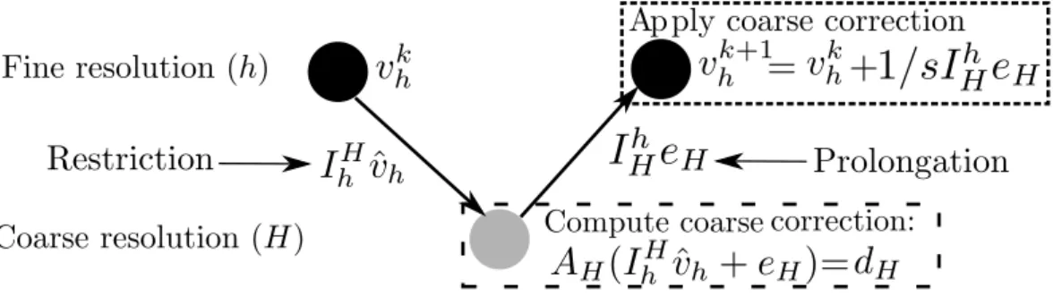
3.4 Analysis of the Full Approximation Scheme . . . 75
3.4.1 Prolongation and Restriction . . . 75
3.4.2 The FAS Algorithm . . . 77
3.4.3 Numerical Example from a Multiscale Manufacturing System . . . 78
CONTENTS 19
3.5 The Alternating Multiresolution Scheme . . . 83
3.5.1 One-way Multiresolution Scheme . . . 84
3.5.2 Convergence Analysis of AMS . . . 90
3.6 Action Space Sampling for the Coarse Model . . . 100
3.6.1 Linear Programming and MDPs . . . 100
3.7 Numerical Experiments . . . 104
3.7.1 Manufacturing Example . . . 105
3.7.2 Example from Molecular Dynamics . . . 106
3.8 Discussion . . . 109
4 Empirical Risk Minimization: Probabilistic Complexity and Stepsize Strat-egy 110 4.1 Introduction . . . 111
4.2 Preliminaries . . . 115
4.3 Complexity Analysis using Random Matrix Theory . . . 117
4.3.1 Statistical Bounds . . . 118
4.3.2 Complexity Analysis . . . 126
4.4 PUG: Probabilistic Upper-bound Guided stepsize strategy . . . 128
4.4.1 Current Stepsize Strategies . . . 129
4.4.2 PUG . . . 131
4.4.3 Convergence Bounds: Regular Strategies vs. PUG . . . 133
4.5 Numerical Experiments . . . 135
4.5.1 Numerical Simulations for Average L . . . 135
4.5.2 Regularized Logistics Regression . . . 136
4.5.3 Regularized Linear Regression . . . 138
4.6 Conclusions and Perspectives . . . 138
5 Multilevel Methods for Unconstrained Convex Optimization 140 5.1 Introduction . . . 140
5.2 Multilevel Models . . . 144
5.2.1 Basic Settings . . . 145
5.2.2 The General Multilevel Algorithm . . . 147
5.2.3 Connection with Variable Metric Methods . . . 151
5.2.4 Connection with Block-coordinate Descent . . . 152
5.2.5 Connection with SVRG . . . 153
5.2.6 The Galerkin Model . . . 154
5.3 Convergence of GAMA . . . 155
5.3.1 The Worst Case O(1/k) Convergence . . . 157
5.3.2 Maximum Number of Iterations of Coarse Correction Step . . . 162
5.3.3 Quadratic Phase in Subspace . . . 164
5.3.4 Composite Convergence Rate . . . 167
5.4 Complexity Analysis . . . 172
CONTENTS 21
5.4.2 Complexity Analysis: GAMA . . . 176
5.4.3 Comparison: Newton v.s. Multilevel . . . 183
5.5 PDE-based Problems: One-dimensional Case . . . 185
5.5.1 Galerkin Model by One-dimensional Interpolations . . . 186
5.5.2 Analysis . . . 187
5.5.3 Convergence . . . 192
5.6 Low Rank Approximation using Nystr¨om Method . . . 193
5.6.1 Galerkin Model by Na¨ıve Nystr¨om Method . . . 194
5.6.2 Analysis . . . 196
5.6.3 Convergence . . . 199
5.7 Block Diagonal Approximation . . . 202
5.7.1 Multiple Galerkin Models . . . 203
5.7.2 A Counterexample for General Functions . . . 204
5.7.3 Weakly connected Hessian . . . 205
5.7.4 Analysis . . . 205
5.7.5 Convergence . . . 208
5.8 Numerical Experiments . . . 210
5.8.1 Poisson’s Equation . . . 210
5.8.2 Regularized Logistic Regression . . . 212
5.8.3 A Synthetic Example for Block Diagonal Approximation . . . 213
5.9 Comments and Perspectives . . . 219 6 Discussion 221 6.1 Summary . . . 221 6.2 Future Work . . . 222 Bibliography 223 22
List of Tables
4.1 Gisette . . . 137 4.2 YearPredictionMSDt . . . 137
5.1 PDE-based text examples . . . 216 5.2 Details of ERM Test Examples . . . 217
List of Figures
1.1 The solutions, u(x, y)’s, of the Poisson’s equation (1.1) with different mesh sizes. 28
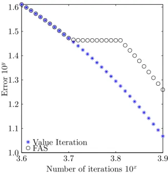
3.1 The Full Approximation Scheme (FAS) . . . 78 3.2 Performance of the FAS,ǫ= 10−2, initial number of iterations in the fine model:
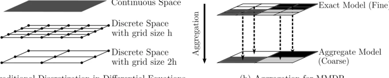
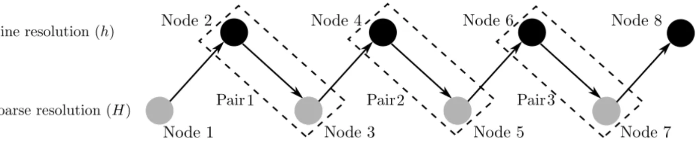
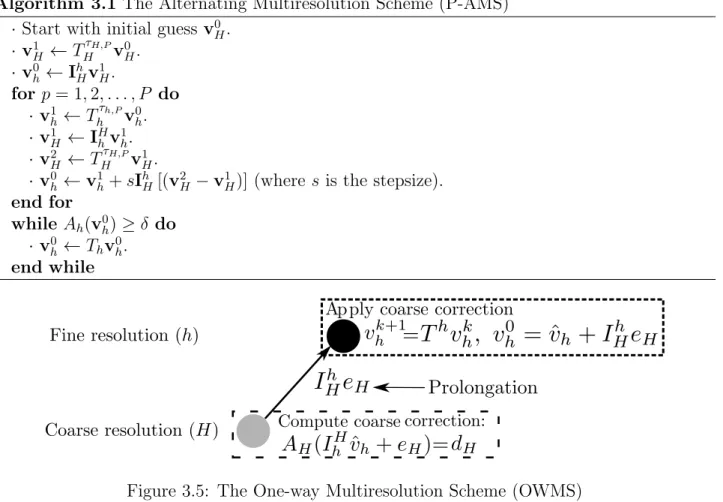
5000, stepsizes = 1. The figure shows that no useful computation is performed by the FAS during the coarse iterations. . . 80 3.3 Different ideas between discretization and aggregation . . . 82 3.4 The Alternating Multiresolution Scheme (AMS) . . . 83 3.5 The One-way Multiresolution Scheme (OWMS) . . . 84 3.6 Stopping criteria in the coarse model . . . 86 3.7 Numerical performance of the different algorithms. Parameters: v0
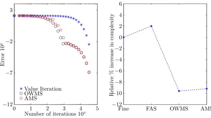
h = 0,v0H = 0,
s = 1.15, and ρ = 0.05. (Left) Iteration History. (Right) Relative increase in realized complexity of the different algorithms. Value iteration was taken to be the base line. Compared to value iteration conventional FAS has an increased complexity, whereas the proposed schemes achieve a 10% reduction. . . 106 3.8 Numerical results of different algorithms. Parameters: v0
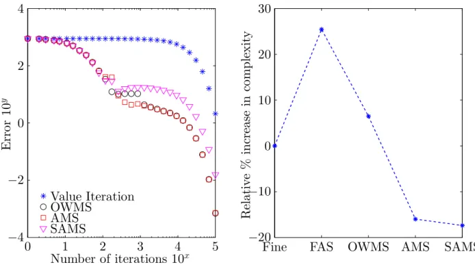
h = 0, v0H = 0, s= 1.1,
R= 10000, andρ= 0.05. (Left) Convergence in each iteration. (Right) Relative increase in realized complexity of the different algorithms. Value iteration was taken to be the base line. . . 108
4.2 Case II, 2m =n . . . 135 4.3 Case III, n= 1024 . . . 135
5.1 Pin (5.25) . . . 186 5.2 R in (5.26) . . . 186 5.3 Φ(σ2) in (5.33) . . . 200
5.4 Convergence of solving Poisson’s equation with different N’s . . . 211 5.5 The smoothing effect with different N’s . . . 211 5.6 The ℓ1 regularized logistic regression example. . . 213
5.7 Block diagonal approximation. . . 214 5.8 YearPredictionMSDt . . . 220 5.9 log1pE2006test . . . 220 5.10 w8at . . . 220 5.11 Gisette . . . 220 5.12 epsilon normalizedt . . . 220 5.13 epsilon normalizedt (subsample) . . . 220
Chapter 1
Introduction
I don’t know anything, but I do know that everything is interesting if you go into it deeply enough.
Richard Feynman
1.1
Motivation and Objectives
Due to the complexity of practical applications, the ability to solve large scale optimization problems is crucial. Examples can be found across many disciplines: machine learning [SNW12], finance [Pri07], logistics [YCYA12], energy systems [PW14], molecular conformation [Wu96]. As one of the fundamental challenges in computational science, solving large scale optimization is computationally demanding, and much efforts have been made to reduce this burden. In general, it is fair to say that solving an arbitrary optimization problem could be very difficult, or it simply could not be done [BV04]. Problems arising from practical applications, however, often have particular structure. In what follows, we will discuss several important applications and their underlying structure.
1 0.8 0.6 0.4 x 0.2 0 0 y 0.5 1 0.5 0 -0.5 -1 1 u ( x ;y ) 1 0.8 0.6 0.4 x 0.2 0 0 y 0.5 -1 -0.5 0 0.5 1 1 u ( x ;y )
Figure 1.1: The solutions, u(x, y)’s, of the Poisson’s equation (1.1) with different mesh sizes.
Geometric Structure
Many optimization problems exhibit geometric structure, in which the geometry of the solution can be approximated.
One classical example is the class of infinite-dimensional optimization problems, which include many problems in optimal control. These problems usually could not be solved exactly, and one needs to approximate and discretize the original problem using finite differences or finite elements. The dimension of the discretized problem depends on the mesh size during the discretization. In general, smaller mesh size results in higher dimensional problems, although the solution would be more accurate. Figure 1.1 shows an example using a two-dimensional Poisson’s equation, −∂ 2u ∂x2 − ∂2u ∂y2 = 13π
2sin(2πx) sin(3πy), in Ω = [0,1]2, (1.1)
where,
u= 0, on ∂Ω.
Notice that the “two-dimensional” in (1.1) refers to the dimensions of the continuous variables in the original Poisson’s equation, i.e. x and y. Once the Poisson’s equation is discretized, the decision variable of the corresponding optimization problem is not in two dimensions, and the number of dimensions is the same as the number of grid points on the chosen mesh. Figure
1.1. Motivation and Objectives 29 1.1 shows the solutions of a Poisson’s equation using different mesh sizes. One can see that although using a large mesh size would yield an inaccurate solution, the geometry of the solution is highly similar to the solution which is computed by using a smaller mesh size. Thus, the geometric structure of the solution is preserved across the different mesh sizes.
Another example can be found in image processing. For natural images, it is expected that the same image with different resolutions would have the same structure for every small region of the image. That is, neighbouring pixels usually have similar image intensities. Therefore, one can use a high resolution image to construct a low resolution image that is visually similar. For applications such as image de-blurring, images with lower resolution would yield an optimization model that is in lower dimension [PLRR].
Multiscale Structure
Apart from geometric structure, many practical applications on complex systems present mul-tiscale structure, i.e. there exists an important feature in which its magnitude spans across multiple scales, such as time and space scales.
One important example could be found in energy systems, where many long term sequential decisions are made based on the dynamics of an environment. This environment depends on the long term decisions made as well as the short-term operations such as unit commitment and generation dispatch. The interactions between long term environment and short term operations display a multiple time scales dynamics, i.e. dynamics that evolve significantly in both short and long time horizons [PW14].
The resource allocation problem in cloud provisioning is another example [MKC13, KRC+15]. Cloud provisioners often receive job requests that have needs for a certain amount of cloud resource within a time period. These requests could ask for cloud resource that ranges from the scale of 10 units to 10000 units, and so the resource requirement of this problem exhibits a multiscale structure. On the other hand, the deadlines of these job requests also have multiscale structure since they could be in the range of seconds to hours, or even days.
Statistical Structure
Consider an example in stochastic optimization,
min
x∈RnEQ[f(x,ξ)], (1.2)
whereξ∈RP is a random vector which follows the distributionQ, andf is convex inx. There-fore, the above optimization model minimizes the expected value of f with decision variable
x. In practice, however, the distribution Q is often unknown. Instead, one is usually given a sample of data, i.e. {ξi}mi=1. In such cases, one common way is to solve the sample average of the above optimization model, i.e.
min x∈Rn 1 m m X i=1 fi(x), (1.3) where fi(x) =f(x,ξi), fori= 1,2, . . . , m.
Equation (1.3) is called the Sample Average Approximation (SAA), and SAA has a long history of developments. See [BL11, KSHdM02] for more details. One famous example of using SAA is the empirical risk minimization, which is a general form of many popular regression models, including linear regression and logistics regression.
Notice that SAA (1.3) displays a unique statistical and mathematical structure. Firstly, SAA always has the form of a sum of functions. Secondly, the difference between each fi is due to the data pointsξi’s, in which they follow the same probability distribution. These two features of SAA have motivated a lot of development in optimization algorithms, including stochastic gradient descent [Bot12, PJ92, TH12, Bot98] and mini-batch algorithms [CR16].
In this thesis, we aim to take advantages of problem structure to advance computational per-formance of optimization algorithms. The structure of this thesis will be provided in the next section.
1.2. Thesis Outline and Contributions 31
1.2
Thesis Outline and Contributions
We consider optimization problems with different structures, and develop efficient algorithms based on this additional information. The problems we consider cover a large spectrum of in-teresting applications, ranging from stochastic optimal control to machine learning to infinite-dimensional optimization. Except for Section 4, the main approach used is multilevel optimiza-tion methods, which follow the idea of multigrid methods for solving (non-)linear equaoptimiza-tions of discretizations arising from partial differential equations. This thesis expands the capabilities and knowledge in the field of multilevel optimization methods.
Apart from Chapter 2 and Chapter 6, which we provide the background materials and the conclusions, this thesis is divided into three parts. Each part corresponds to a class of structured optimization problems.
In Chapter 3, we consider singularly perturbed Markov Decision Processes (MDPs), which exhibit multiple time-scale structure. An existing result shows that a singularly perturbed MDP could be approximated by an aggregate model. The solution of the aggregate model was shown to be asymptotically optimal [YZ13]. By making use of this result, a multilevel algorithm is developed by replacing some parts of the computation using the coarse model. We show that the complexity of the proposed algorithm is superior to the standard value iteration for this class of problems. The contents of this chapter appeared in the following paper:
1. C. P. Ho, and P. Parpas. Singularly Perturbed Markov Decision Processes: A Multireso-lution Algorithm. SIAM Journal on Control and Optimization 52:6, 3854-3886, 2014.
In Chapter 4, we consider the computational complexity and stepsize strategy of regularized empirical risk minimization problems. The worst-case complexity for this problem follows from standard results in convex optimization theory [BT09, Nes15]. Some algorithms in this class of problems are considered to be “dimension-free” because the convergence analysis of these algorithms is independent of the size of the problem. This above argument is based on the as-sumption that the Lipschitz constant of the problem is independent of the dimensionality. We
show that the dimensionality of the model is, however, hidden within the Lipschitz constant. Standard random matrix theory is used to derive the probabilistic bounds of the Lipschitz con-stant. The derived bounds are also used to develop a stepsize strategy for better computational performance. The contents of this chapter are currently being prepared for publication with the following working title:
2. C. P. Ho, and P. Parpas. Empirical Risk Minimization: Probabilistic Complexity and Stepsize Strategy. In preparation.
In Chapter 5, we consider the unconstrained convex optimization problem. We provide a broader view on the general multilevel framework, and we show a connection between this framework and standard optimization methods. A special case of this general framework is further studied, and we call it Galerkin-based Algebraic Multilevel Algorithm (GAMA). The Galerkin model is highly related to algebraic multigrid methods, in which the hierarchy of the models is generated by using the algebraic information of the models instead of using the geometric structure. In the view of optimization, GAMA is equivalent to performing Newton’s method in reduced dimensions. We prove that GAMA has a local rate of composite convergence, which is a linear combination of linear and quadratic convergence. By considering three case studies, we show how the structure of the problems could affect the convergence of multilevel methods. The contents of this chapter are currently being prepared for publication with the following working title:
3. C. P. Ho, and P. Parpas. Multilevel Optimization Methods: Convergence and Problem Structure. In preparation.
During the 4 years of doctoral studies, I was fortunate to have opportunities to collaborate with different researchers and PhD students at Imperial College London. Below is a list of publications which do not directly contribute to this thesis.
4. X. Chen, C. P. Ho, R. Osman, P. Harrison, and W. Knottenbelt. Understanding, Mod-elling and Improving the Performance of Web Applications in Multi-core Virtualised
Envi-1.2. Thesis Outline and Contributions 33
ronments. Proceedings of the 5th ACM/SPEC International Conference on Performance Engineering (ICPE) 197-207, 2014.
5. C. P. Ho, and P. Parpas. On Using Spectral Graph Theory to Infer the Structure of Multiscale Markov Processes. 2015 Proceedings of the Conference on Control and its Applications 228-235, 2015.
6. L. Chen, T. Tong, C. P. Ho, R. Patel, D. Cohen, A. C. Dawson, O. Halse, O. Geraghty, P. E.M. Rinne, C. J. White, T. Nakornchai, P. Bentley, and D. Rueckert. Identifica-tion of Cerebral Small Vessel Disease Using Multiple Instance Learning. Medical Image Computing and Computer-Assisted Intervention MICCAI 2015, Springer International Publishing, 9349, 523-530, 2015.
7. Y. Li, C. P. Ho, N. Chahal, R. Senior, and M.-X. Tang. Myocardial Segmentation of Contrast Echocardiograms Using Random Forests Guided by Shape Model. Accepted for Medical Image Computing and Computer-Assisted Intervention MICCAI, 2016.
Background Theory
It is not knowledge, but the act of learning, not possession but the act of getting there, which grants the greatest enjoyment.
Carl Friedrich Gauss
In this chapter, we will provide background material for the thesis. The chapter is divided into three sections.
In the first section, we review first order and second order algorithms which solve unconstrained continuous convex optimization problems. We consider the conventional setting that the objec-tive function is (twice) continuously differentiable and Lipschitz continuous, and we introduce four classical algorithms: gradient descent, block-coordinate descent, Newton’s method, and quasi-Newton methods. We also consider the composite convex program, in which the ob-jective function is a sum of a continuously differentiable function and a simple function. The definition of simple function will be provided later in the section. One state-of-the-art algorithm for such problems is known as “FISTA”, which stands for Fast Iterative Shrinkage-Thresholding Algorithm. Algorithmic details and theoretical performance of all five algorithms will be re-viewed.
2.1. Unconstrained Continuous Convex Optimization 35 In the second section, some existing results in machine learning and statistics are provided, and these results will be used later in this thesis. We first summarize some concentration bounds in both random variables and random matrices. We then introduce the Nystr¨om method, which is used to compute low rank approximations of positive semi-definite matrices.
In the third section, we review background materials for Markov decision processes (MDPs). We cover the basis of continuous-time Markov chains (CTMCs), Markov decision processes (MDPs), and the two common computational methods for MDPs: value iteration and linear programming.
We emphasize that each topic covered in this chapter has its own long history in research, and this chapter is far from a complete review of all of them. The goal of this chapter is to cover necessary knowledge that will lead to a smoother reading experience for the rest of this thesis. The material presented in this chapter is based on [BT09, BT13, BV04, Ros06, Pow11, Tro15, PGD+15, Git11, NW06].
2.1
Unconstrained Continuous Convex Optimization
In this section we are interested in the unconstrained continuous convex program,
min
x∈Rnf(x), (2.1)
where f :Rn→R is a convex function. Note that we require different additional properties of a convex function at different stages of this thesis. Below is a list of common properties.
Definition 2.1 A continuously differentiable functionf :Rn →Ris said to have aL-Lipschitz continuous gradient if
Suppose f is also twice continuously differentiable. Then the above definition is equivalent to
−LI ∇2f(x)LI, ∀x∈Rn.
Definition 2.2 A twice continuously differentiable function f : Rn → R is said to have a
M-Lipschitz continuous Hessian if
k∇2f(x)− ∇2f(y)k ≤Mkx−yk, ∀x,y∈Rn.
Definition 2.3 A convex differentiable function f : Rn → R is said to be strongly convex if there exists a positive constant µ such that for each x∈Rn,
f(y)≥f(x) +∇f(x)T(y−x) +µky−xk2, ∀y∈Rn.
Suppose f is also twice continuously differentiable. Then the above definition is equivalent to
µI ∇2f(x), ∀x∈Rn.
2.1.1
First Order Methods
We begin with the introduction of first order methods. Starting with the case that the objective function is differentiable and has a L-Lipschitz continuous gradient, gradient descent method and block-coordinate descent method are introduced. We then consider objective functions that have the form of a composite function, i.e. a sum of a differentiable function and a (non-smooth) simple function. In such setting, we introduce one standard first order method - Fast Iterative Shrinkage-Thresholding Algorithm (FISTA) [BT09]. FISTA can be seen as an extension of gradient descent method with two main differences: (i) Nesterov’s acceleration techniques [Nes04] is applied for FISTA. (ii) It accommodates for composite functions.
2.1. Unconstrained Continuous Convex Optimization 37
Gradient Descent
Consider the objective function
min
x∈Rnf(x), (2.2)
wheref is a continuously differentiable function and hasL-Lipschitz continuous gradient. Gra-dient descent is an iterative method for (2.2). For any initial guessx0, it updates the incumbent by
xk+1=xk+αkdk, k = 0,1,2, . . . ,
where αk ∈Rand dk∈Rn are the stepsize and direction at the kth iteration, respectively. The idea of gradient descent is to use the negative gradient as the direction,
dk =−∇f(xk),
and this particular choice of direction is a descent direction, since
∇f(xk)Tdk=−k∇f(xk)k2 <0, ∀∇f(xk)6= 0.
There are many methods to compute stepsize αk. When L is known or could be estimated, then one choice could be αk = 1/L since
f xk− 1 L∇f(xk) ≤ f(xk) +∇f(xk)T −1 L ∇f(xk) +L 2 1 L∇f(xk) 2 = f(xk)− 1 Lk∇f(xk)k 2 + 1 2Lk∇f(xk)k 2 = f(xk)− 1 2Lk∇f(xk)k 2.
That is, the next incumbentxk+1 has a smaller function value as long as∇f(xk)6= 0. However, in many casesL is unknown, and one needs to use a large enough constant ˜Lk such that,
f xk+ 1 ˜ Lk dk ≤f(xk)− 1 2 ˜Lk k∇f(xk)k2. (2.3)
Algorithm 2.1 Gradient descent
Input parameters: Initial guess x0 ∈Rn, η >1. Choice of Option 1 or 2.
for k = 1,2,· · · do
Compute the direction dk =−∇f(xk). Select αk using
❼ Option 1: αk = 1/L.
❼ Option 2: Find the smallest q∈N such that for ˜Lk =ηqL˜k−1, ˜Lk satisfies (2.3). Set
αk = 1/L˜k. Set xk+1 =xk+αkdk.
end for
Algorithm 2.1 provides the details of gradient descent method. The following theorem states the theoretical performance of gradient descent.
Theorem 2.4 ([Nes04]) Suppose Algorithm 2.1 is performed, then
f(xk)−f(x⋆)≤ Lˆkx0−x⋆k 2 2k ,
where Lˆ =L if Option 1 is chosen, and Lˆ =ηL if Option 2 is chosen.
From Theorem 2.4, one can see the function value converges to the minimum at a rate in
O(1/k). We emphasize that gradient descent method is not the best among its kind. In particular, Nesterov proposed the optimal scheme, which accelerates gradient descent method to the rate in O(1/k2) [Nes04].
Block-coordinate Descent
When using Algorithm 2.1 to solve (2.2), gradient evaluations and vector operations are needed. However, these operations could be computationally expensive or even intractable for large scale problems. To this end, block-coordinate descent methods were proposed to relax this computational burden. Similar to gradient descent method, block-coordinate descent can be
2.1. Unconstrained Continuous Convex Optimization 39 accelerated using the Nesterov’s acceleration techniques [BT13]. However, for the purpose of this thesis, we shall focus on the non-accelerated version.
The basic idea of block-coordinate descent is to decompose vector operations. We denote matrices Ui ∈Rn×ni,i= 1, . . . , p, for which
[U1U2. . .Up] =I,
whereni’s are positive integers such thatPpi=1ni =n. The above notation considers a division of p blocks, and each i represents the ith block. Using the notation of U
i, we define the ith block of the gradient
∇if(x),UTi ∇f(x).
For block-coordinate descent, we further assume thatf is block-wise Lipschitz continuous, i.e. there exist constants Li, i= 1,2, . . . , p such that
k∇if(x+Uihi)− ∇if(x)k ≤Likhik, ∀hi ∈Rni.
Following the above notation, we can define theith block of gradient update in thekth iteration
xik =xik−1− 1
Li
Ui∇if(xik−1).
The above update uses the stepsize 1/Li. When Li is unknown, one can apply the same technique as in gradient descent, i.e. finding a large enough ˜Li such that
f xik−1− ˜1 Li Ui∇if(xik−1) ≤f(xik−1)− 1 2 ˜Li k∇if(xik−1)k2. (2.4) Algorithm 2.1 states the algorithmic procedure of block-coordinate descent method. The theoretical performance is provided in the following theorem, and it uses following notations.
X⋆ , n x⋆ :x⋆ ∈arg min x∈Rnf(x) o , and R(x0),max x∈Rnx⋆max∈X⋆{kx−x⋆k:f(x)≤f(x0)}.
Algorithm 2.2 Block-coordinate gradient descent
Input parameters: Initial guessx0 ∈Rn, (For option 2: L0j, j = 1, . . . , p). Choice of Option 1 or 2.
for k = 1,2,· · · do
Set x0k =xk and update recursively
xik=xik−1−αikUi∇if(xik−1), i= 1, . . . , p, where αi
k is computed by ❼ Option 1: αi
k = 1/Li
❼ Option 2: Find the smallest q ∈ N such that for ˜Li = ηqL˜0i, ˜Li satisfies (2.4). Set
αk = 1/L˜i. Set xk+1 =xpk.
end for
Theorem 2.5 ([BT13]) Suppose Algorithm 2.2 is performed. Then for k= 0,1, . . . ,
f(xk)−f(x⋆)≤ 4Lmax(1 +p3κ2)R2(x0) 1 k+ (8/p) if Option 1, 4ηLmax(1 +pL2/(L0 min)2)R2(x0) 1 k+ (8/p) if Option 2,
where Lmax= maxiLi, κ= (maxiLi)/(miniLi), L0min = miniL0i.
From Theorem 2.5, one can see the drawback of block-coordinate descent method because pis inversely proportional to the performance of the algorithm. That is, the more blocks we make, the worse rate of convergence block-coordinate descent would have. Therefore, for problems in which vector operations and gradient evaluations are not computationally expensive, gradient descent would be preferable.
FISTA
We now let the objective function to be in the form of a composite function. That is,
min
2.1. Unconstrained Continuous Convex Optimization 41 wheref :Rn →Ris a convex function withL-Lipschitz continuous gradient, andg :Rn→Ris a continuous convex function which is possibly nonsmooth but simple. The definition of simple function means that it results in computationally inexpensive proximal projection steps, which will be formally defined later in this section.
One of the standard optimization algorithms for (2.5) is FISTA. FISTA is a modification of ISTA, Iterative Shrinkage-Thresholding Algorithm, with the additional Nesterov’s acceleration technique applied [Nes04]. For both FISTA and ISTA, the proximal projection step is taken in each iteration pL(y),arg min{QL(x,y) :x∈Rn}, where QL(x,y),f(y) +hx−y,∇f(y)i+L 2kx−yk 2+g(x).
We point out the the proximal projection step admits a unique minimizer. Recall that g is assumed to be a simple function. By simple we mean that the choice ofg would yield to cheap computation in the “arg min” procedure at the proximal steppL(·). One special case ofg is the weighted ℓ1 norm. Suppose g(x) = ωkxk1 with positive constant ω, the proximal step would become pL(y) =Tω/L x− 1 L∇f(x) ,
where Tα is called the shrinkage operator, and
Tα(x)i = (|xi| −α)+sgn(xi).
One can see that in this special case the proximal step is no more than a usual gradient descent step plus the shrinkage operator, which is computationally inexpensive.
The details of FISTA with constant stepsize are provided in Algorithm 2.3. Notice that Algo-rithm 2.3 requires the Lipschitz constant L. When L is not known, one has to ensure at each iteration, a large enough ˜L is chosen. In particular, at the kth iteration with incumbent xk, ˜L
Algorithm 2.3 FISTA with constant stepsize
Input parameters: Lipschitz constant L, initial guessx0 ∈Rn.
Initialization: Set y1 =x0 and t1 = 1.
for k = 1,2,· · · do xk = pL(yk), tk+1 = 1 +p1 + 4t2 k 2 , yk+1 = xk+ tk−1 tk+1 (xk−xk−1). end for
Algorithm 2.4 FISTA with backtracking
Input parameters: Initial guess x0 ∈Rn, L0 >0,η >1
Initialization: Set y1 =x0 and t1 = 1.
for k = 1,2,· · · do
Find the smallest q∈N such that for ˜L=ηqL k−1,
F(pL˜(xk))≤QL˜(pL˜(xk),xk). Set Lk =ηqLk−1 and compute
xk = pLk(yk), tk+1 = 1 +p1 + 4t2 k 2 , yk+1 = xk+ tk−1 tk+1 (xk−xk−1). end for
needs to be large enough to satisfy
F(pL˜(xk))≤QL˜(pL˜(xk),xk).
Algorithm 2.4 provides the details of FISTA with backtracking stepsize strategy. We should mention that the stepsize strategy in Algorithm 2.4 is the original approach proposed in [BT09], but not the only one. See for example [Nes15].
2.1. Unconstrained Continuous Convex Optimization 43
Theorem 2.6 Suppose Algorithm 2.3 or 2.4 is performed. Then for any k ≥1,
F(xk)−F(x⋆)≤ 2 ˆLkx0−xkk 2 (k+ 1)2 ,
where x⋆ = arg minxF(x), Lˆ =L if the constant stepsize strategy is chosen, and Lˆ =ηL if the
backtracking stepsize strategy is chosen. η is the user-defined parameter in Algorithm 2.4.
Both versions of FISTA have optimal theoretical performance guarantees. Compared to the non-accelerated version ISTA which has the rate O(1/k), FISTA converges with the rate
O(1/k2), as stated in Theorem 2.6.
We emphasize that research in first order algorithms is a popular topic. Gradient descent, block-coordinate descent, and FISTA are just three standard algorithms. We refer readers to [RT16, HPZ15, DBLJ14, HL15, Nes04, Nes15, LPRR16, BTMN01] for the developments on this line of research, including Nesterov’s acceleration technique, mirror descent, and parallel coordinate descent.
2.1.2
Second Order Methods
In the rest of this section, some background material on second order algorithms is provided. We solely consider second order methods that solve problems in the following form
min
x∈Rnf(x), (2.6)
where f is a twice continuously differentiable function. We further assume thatf is a strongly convex function with parameter µ, and f hasL-Lipschitz continuous gradient andM-Lipschitz continuous Hessian.
The above setting is more restrictive compared to (2.2) because of the extra assumptions on strong convexity and twice differentiability. Countless research studies have been conducted on solving (2.6), and it is impossible to mention every one of them. We refer readers to
[DM77, DES82, Ber95, NW06] for more details. However, it is fair to say that a good portion of those algorithms are variants of Newton’s method. In what follows, we will provide the details of Newton’s method and one of its variants, quasi-Newton method.
Newton’s method
Similar to the gradient and block-coordinate descent, Newton’s method is an iterative method. The core idea of Newton’s method is based on second order approximation of f at the current incumbent xk, i.e.
f(xk+d)≈f(xk) +h∇f(xk),di+ 1 2d
T∇2f(xk)d,
and the directiondk is computed by minimizing the right hand side of the above equation over
d. Equivalently,
dk=−[∇2f(xk)]−1∇f(xk).
There are many methods to compute stepsize αk, but for the purpose of this chapter, we only consider the Armijo’s rule, i.e., we require that αk satisfies
f(xk+αkdk)≤f(xk) +ρ1αk∇f(xk)Tdk. (2.7) where ρ1 ∈ (0,0.5) is a user-defined parameter. The Armijo’s rule ensures the stepsize yields a sufficient reduction in function value. In particular, the next function value f(xk+1) must be less than f(xk), since dk is a descent direction and ∇f(xk)Tdk≤0.
Algorithm 2.5 is one standard version of Newton’s method using Armijo’s rule as stepsize strategy. In the following two theorems, we state the theoretical performance of Newton’s method.
Theorem 2.7 ([BV04]) Suppose Algorithm 2.5 is performed and k∇f(xk)k ≥ η, for some
η >0, then
f(xk+1)−f(xk)≤ −ρ1βlsη2
µ L2.
2.1. Unconstrained Continuous Convex Optimization 45
Algorithm 2.5 Newton’s method with Armijo’s rule
Input parameters: Initial guess x0 ∈Rn, ρ1 ∈(0,1/2), βls ∈(0,1)
for k = 1,2,· · · do
Compute the direction
dk =−[∇2f(xk)]−1∇f(xk). Find the smallest q∈N such that forαk =βlsq,
f(xk+αkdk)≤f(xk) +ρ1αk∇f(xk)Tdk. Set xk+1 =xk+αkdk.
end for
Theorem 2.8 ([BV04]) Suppose Algorithm 2.5 is performed and k∇f(xk)k ≤3(1−2ρ1)
µ2 M, then k∇f(xk+1)k ≤ M 2µ2k∇f(xk)k 2.
Theorem 2.7 and 2.8 describe the performance of Newton’s method at different stages. Suppose when the current incumbent xk is far from the solution x⋆, Theorem 2.7 guarantees that each iteration of Newton’s method would result in a reduction in function value, and thus moving closer to x⋆. This stage is called the damped Newton phase. Once the current incumbent
xk is sufficiently close to x⋆, i.e. k∇f(xk)k is sufficiently small, Theorem 2.8 guarantees that the norm of the gradient would be reduced quadratically in each iteration. This stage of the iterative process is called the quadratically convergent phase.
We emphasize that the quadratically convergent phase is the main reason that Newton’s method outperforms many other algorithms. However, the drawback of using Newton’s method is clear: one needs to solve an×nsystem of linear equations in each iteration. For large scale problems with large n, Newton’s method is intractable. Despite its obvious limitation, Newton’s method is one of the best algorithms for moderate size optimization problems, and it serves as a base case for many further developments in unconstrained continuous optimization, including the two well-known types of algorithms: inexact Newton method and quasi-Newton method.
Quasi-Newton methods
Quasi-Newton methods were developed to overcome the major drawbacks of Newton’s method: evaluation of Hessians and expensive iteration cost. The main idea of quasi-Newton methods is to approximate Newton steps using just first order information. In what follows, we provide the background materials of the BFGS method, which is the most popular quasi-Newton method. BFGS is named after Broyden, Fletcher, Goldfarb, and Shanno. We then discuss the drawback of BFGS, and how it could be relaxed by the limited-memory BFGS (L-BFGS). L-BFGS is one of the state-of-the-art methods for unconstrained optimization.
Consider the problem (2.6), at the kth iteration, the direction of using Newton’s method is computed by minimizing the following model,
dk = arg min d∈Rnf(xk) +h∇f(xk),di+ 1 2d T ∇2f(xk)d.
The basic idea of BFGS is to consider an approximation of the Hessian using the model,
mk(d) =f(xk) +h∇f(xk),di+ 1 2d
TB kd,
for a symmetric positive definite matrix Bk. Notice thatBk is analogous to ∇2f(xk), as shown above. When using the BFGS method, the approximation of the Hessian is not computed afresh at every iteration, but rather it is updated using the previous estimate in the last iteration. In order to do so, one has to impose the updating rules at each iteration. In the case of BFGS, it is based on the idea of secant equation,
∇mk+1(−αkdk) = ∇f(xk).
The secant equation is based on the observation that ∇mk+1(0) = ∇f(xk+1). If the secant equation is satisfied, then the model mk+1 is a good interpolation of the objective functionf, and it has gradients that are matched at the points xk and xk+1. The above secant equation
2.1. Unconstrained Continuous Convex Optimization 47 can be re-written as,
Bk+1sk =yk,
where sk , xk+1 −xk and yk , ∇f(xk+1)− ∇f(xk). Using the idea of the above secant equation, we then can approximate the inverse of the Hessian [∇2f(xk+1)]−1 by,
sk =Hk+1yk, (2.8)
where Hk+1 =B−k+11 and so it is analogous to [∇2f(xk+1)]−1.
Equation (2.8) states the constraints when one updates the inverse of the Hessian. In the BFGS method, one updates the Hk+1 based on the following optimization problem [NW06].
min
H kH−HkkG˜k (2.9)
subject to H=HT, Hyk =sk,
where kAkW ,kW1/2AW1/2kF for all matrix that satisfy Wsk =yk, and ˜ Gk = Z 1 0 ∇ 2f(x k+τ αkdk) dτ.
The optimization problem (2.9) has a unique analytical solution
Hk+1 = (I−ρkskyTk)Hk(I−ρkyksTk) +ρksksTk, (2.10) where ρk = 1/yTksk. This above update is the core step in BFGS, and it is used to update the approximation of inverse Hessian at each iteration.
Algorithm 2.6 provides the algorithmic procedure of BFGS method. The theoretical advantage of BFGS is stated in the following theorem.
Algorithm 2.6 BFGS method
Input parameters: Initial guess x0 ∈ Rn, ρ1 ∈ (0,1/2), βls ∈ (0,1), H0 ∈ Rn×n which is symmetric and positive definite.
for k = 0,1,2,· · · do
Compute the direction
dk =−Hk∇f(xk). Find the smallest q∈N such that forαk =βlsq,
f(xk+αkdk)≤f(xk) +ρ1αk∇f(xk)Tdk. Set xk+1 =xk+αkdk.
Update Hk+1 using BFGS update (2.10).
end for
to the minimizer x⋆ of f. In particular, it converges at a superlinear rate. That is,
kxk+1−x⋆k ≤o(kxk+1−x⋆k), as k→ ∞. The above definition of superlinearly convergence was taken in [DES82].
From Algorithm 2.6, one can see that BFGS requires a large amount of storage for the inverse Hessian Hk and requires a matrix-vector multiplication at each iteration. These requirements are not ideal when n is large. To reduce these computational burdens, limited-memory BFGS method was developed.
L-BFGS avoids the storage of the inverse Hessian by the following observation. From equation (2.10), one can rewrite the BFGS update as
Hk+1 =VTkHkVk+ρksksTk,
where Vk = I−ρkyksTk. By recursively applying the above updating equation m times, for some positive integerm, L-BFGS could store the approximation ofHkimplicitly by just storing the m lastest pairs of si and yi.
Algorithm 2.7 states the details of how L-BFGS computes the direction dk using two-loop recursion. Notice that H0
k in Algorithm 2.7 is often chosen to be the identity matrix. In this case one can see that L-BFGS has the computational advantage of only performing vector
2.2. Machine Learning and Statistics 49
Algorithm 2.7 L-BFGS direction update (at the kth iteration)
Input: ∇f(xk),{si,yi}i=kk−1−m, and H0k ∈Rn×n which is symmetric and positive definite. Set qk−1 =∇f(xk). for i=k−1, k−2, . . . , k−m do Update βi =ρisTi qi. Update qi−1 =qi−βiyi. end for Set ˜dk−m =H0kqk−m−1. for i=k−m, k−m+ 1, . . . , k−1do Update ζi =ρiyTi d˜i. Update ˜di+1 = ˜di−si(βi−ζi). end for Output: direction dk =−d˜k.
operations, and matrix operations are completely avoided. This is done by computing the approximation of the direction−[∇2f(xk)]−1∇f(xk) at once instead of having the two separate steps - approximating the inverse Hessian and then computing the direction.
We refer the readers to [BV04, NW06, Ber95] for more details regrading second order methods such as Newton’s method, inexact Newton method, and quasi-Newton method.
2.2
Machine Learning and Statistics
In this section, we review some existing results in machine learning and statistics that serve as tools used in the thesis.
2.2.1
Concentration Bounds
Concentration bounds or concentration inequalities are used to analyze the likelihood of a random variable larger or smaller than some value. In other words, concentration bounds can give the output range of a random variable, with high probability.
In what follows, we will provide some concentration bounds for both scalar random variables and random matrices.
Theorem 2.10 ([Tro11]) Let Q be a finite set of positive numbers, and suppose
max
q∈Q q≤B.
Sample {q1, q2, . . . , ql} uniformly from Q without replacement. Compute
s =l·E(q1). Then P ( X j qj ≤(1−σ)s ) ≤ e−σ (1−σ)1−σ s/B for σ∈[0,1), and P ( X j qj ≥(1 +σ)s ) ≤ eσ (1 +σ)1+σ s/B for σ≥0.
Proof See Theorem 2.1 from Tropp [Tro11].
The above concentration bounds are called Chernoff bounds. We point out that E(q1) =
P
qj∈Qqj/|Q|, since we assume sampling are conducted uniformly without replacement. It shows that, with high probability, the sum of samples over a finite set is bounded by O(l/|Q|), wherelis the size of the subset. We refer reader to [CL06] for other settings apart from sampling uniformly without replacement.
In this thesis, we are only interested in the largest eigenvalue of structured random matrices, which forms the basis of Chapter 4. Below we provide some results from [Tro12] that are used in Chapter 4.
Lemma 2.11 For a sequence {Qk:k = 1,2,· · · , m} of random matrices,
λmax X k E[Qk] ! ≤E " λmax X k Qk !# .
2.2. Machine Learning and Statistics 51
Lemma 2.12 Suppose thatQis a random positive semi-definite matrix that satisfiesλmax(Q)≤
1. Then
EeθQ4I+ (eθ−1)(E[Q]), for θ ∈R,
where I is the identity matrix in the correct dimension.
Lemma 2.13 Consider a sequence{Qk:k = 1,2,· · · , m}of independent, random, self-adjoint
matrices with dimension n. For all t∈R,
P ( λmax m X k=1 Qk ! ≥t ) ≤ninf
θ>0exp −θt+m logλmax 1 m m X k=1 EeθQk !! .
One may find that the above inequality is not meaningful when t is small, i.e. the right hand side is greater than 1 when t is small. However, as we will see in Chapter 4, in this thesis we are interested in the cases wheret is sufficiently large.
2.2.2
The Nystr¨
om Method
We shall first emphasize that originally Nystr¨om method was developed as a numerical method to approximate eigenfunctions [Nys30]. However, the main idea of Nystr¨om method was used to approximate Gram matrix for machine learning applications, and then this name was also used as a computational method for low rank approximation of Gram matrices [WS01]. We clarify that this thesis only considers the latter case.
In the era of big data, storage of matrices becomes a limitation for some applications. Fortu-nately, many matrices that are formed from data exhibit the low rank structure. For a positive semi-definite matrix A ∈ RN×N, its best low rank approximation can be recognized as the following optimization problem
min Aq∈RN×N
kA−Aqk2, s.t. rank(Aq) =q. (2.11) The solution of the above problem, Aq,⋆, is a matrix with rank q. It is obvious that when
q=N, thenAq,⋆ =A. When one restrictsq << N, thenAq,⋆ is the best rankq approximation of the original matrixA. We mention that in the problem (2.11),k · k2 is chosen to be measure of the distance between A and Aq. In general, any measure or norm can be used, but the two most common choices are k · k2 and k · kF.
Whether k · k2 or k · kF is used, an analytical solution of (2.11) is available due to the Eckart-Young-Mirsky theorem [EY36, Mir60]. Denote the eigenvalue decomposition of A as follows,
A=UΣUT = U1 U2 Σ1 Σ2 U1 U2 T (2.12)
where U1 ∈RN×q, U2 ∈ RN×(N−q), Σ1 ∈Rq×q, and Σ2 ∈ R(N−q)×(N−q). We also assume that eigenvalues in Σ are sorted in descending order. Then Aq,⋆ has the form,
Aq,⋆=U1Σ1UT1. (2.13)
We clarify that Eckart-Young-Mirsky theorem applies for the setting in which Adoes not need to be positive semi-definite nor a square matrix, but for the purposes of this chapter we only consider the case where A is positive semi-definite.
From (2.13) one can see that computing the exact solution Aq,⋆ is computationally expensive when N is large, because it requires the eigenvalue decomposition on A. To this end, the Nystr¨om method is developed to compute the approximation ofAq,⋆ and thus a good low rank approximation of A.
The details of Nystr¨om method are provided in Algorithm 2.8, which can also be found in [DM05]. Notice that Aq can be also recognized in the following form,
Aq =AS[STAS]+STA, (2.14)
where S ∈ RN×q such that the ith column of S is the qth
i column of I. One can also notice the advantage of using Nystr¨om’s method in terms of storage. The low rank approximation
2.2. Machine Learning and Statistics 53
Algorithm 2.8 Nystr¨om’s method
Input parameters: A positive semi-definite matrix A∈RN×N
Step 1. Construct a set Q1 ⊆ {1,2,· · · , N}, and let qi be the ith element ofQ1.
Step 2. Construct a matrix A1 ∈Rq×N such that the ith row ofA1 is the qith row of A.
Step 3. Construct a matrixA2 ∈RN×q such that theith column of A2 is theqith column of
A.
Step 4. Construct a matrix A3 ∈Rq×q such that (A3)i,j is (A)qi,qj.
Step 5. Compute Aq=A2A3+A1, whereA+3 is the pseudo-inverse ofA3.
Aq can be stored as three matrices: A1, A2, and A+3. When q ≪ N, the storage requirement of Aq is much less than the original matrix A. Also, the computational cost of performing pseudo-inverse A+3 is not expensive whenq is small.
In general, Q1 is constructed using one of the following methods: i. Uniform sampling (with or without replacement).
ii. Adaptive sampling based on the scores assigned on the columns of A.
iii. Deterministic methods based on the decrease in error,kAq−Ak, by selecting a particular column ofA.
We will focus on the case where uniform sampling without replacement is deployed. This version of Nystr¨om method is called the na¨ıve Nystr¨om’s method.
Theorem 2.14 Let A ∈ RN×N be a positive semi-definite matrix, S ∈ RN×q be a matrix as defined in (2.14), and the eigenvalue decomposition A has the form in (2.12).
Let τ denotes the coherence of U1,
τ =µ0(U1), N
q maxi (U1U T 1)ii.
Then ∀δ, ǫ∈(0,1), suppose
q≥ 2τ klog(k/δ)
(1−ǫ)2 .
The error of using the na¨ıve Nystr¨om method is
kA−Aqk ≤λk+1(A) 1 + N ǫq ,
with probability at least 1−δ, where λk+1(A) is the (k+ 1)th largest eigenvalue of A.
Theorem 2.14 shows the theoretical performance of the na¨ıve Nystr¨om method. As expected, na¨ıve Nystr¨om method achieves good error bound when A has a large spectral gap, i.e. when
λN(A)≤λN−1(A)≤ · · · ≤λk+1(A)≪λk(A)≤ · · · ≤λ1(A).
We refer readers to [DM05, Git13, WS01, SS00] for different versions of Nystr¨om method. Apart from Nystr¨om method, random projection is another technique for low rank approximation. See [HMT11] for a review in details.
2.3
Continuous-Time Markov Decision Processes
Markov decision processes (MDPs) are considered to be one of the standard models for se-quential decision problems under uncertainties. Many practical applications in operations re-search can be categorized as MDPs. Examples include road maintenance [GS97], nuclear plant management [RR95], and revenue management [SSJL99]. To formally define MDPs, we first introduce Markov chains.
2.3.1
Continuous-Time Markov Chains
Continuous-time Markov Chains (CTMCs), by definition, follow the Markov property, i.e. the probability of the future only depends on the current situation but not the past [Ros06]. Every CTMC is constructed by (1) a group of states to illustrate all possible situations in the system
2.3. Continuous-Time Markov Decision Processes 55 and (2) a Markov generator which defines the probabilistic transitions between any two states. We further assume the number of states is always finite. One could refer such Markov chains as discrete-state continuous-time Markov chains.
Suppose we let x(t) to be a CTMC. We can represent the transitions by a matrix called transition probability matrix P(t, s) = (pij(t, s)) where pij(t, s) represents the probability of
x(t) = j given x(s) =i for 0≤s ≤t; that is,
pij(t, s) =P(x(t) = j|x(s) =i).
We should emphasize that, in this thesis, we are only interested in Markov chains that are irreducible, which means it is possible (positive probability) for x(t) to visit any state in the future regardless of the current state. For CTMCs, it is known that all transition probability matrices follow the below differential equation
dP(t, s)
dt = P(t, s)Q(t) , s≤t,
P(s, s) = I.
The matrix Q(t) = (qij(t)) is called the Markov generator which satisfies
qii(t) =−X
j6=i
qij(t) , qij(t)≥0, for j 6=i.
We point out that the diagonal elements of Q(t), qii’s, represent the rates of exiting current state. The off-diagonal elements, qij’s, represent the likelihood that a transition from i to j will occur. Suppose a CTMC is in state i at time 0, it will leave state i at time t where t is a random variable which follows an exponential distribution with parameterqii, and enter a state
j with probability qij/|qii|, ∀j 6=i. In this thesis, we use “x∼Q(t)” to represent the following statement: x(t) is a CTMC in which the uncertainty is govern by the Markov generatorQ(t). The magnitude of Q is related to the “speed” of the process. In general, the larger magnitude represents a faster process. For instance, consider the two Markov generators, Q1 and Q2,
where Q2 = 10Q1. In such case Q1 and Q2 will generate the same Markov processes except the one from Q2 is 10 times faster.
2.3.2
Continuous-Time MDPs
The general goal of Markov Decision Process is to find the best policyuover a Markov process, in which the underlying uncertainties of the process depend partly on the policy. A policy is analogous to a lookup table which suggests an actionaj to each statej in the Markov process. We denote anN state MDP withx(t) and takes values from the state spaceX :={1,2,· · · , N}. For each state i, 1 ≤ i ≤ N, the available actions of the state i are denoted in the set Ai. Therefore, a policy can be described by u = (a1, a2,· · · , aN) where ai ∈ Ai for ∀i ∈ X. The policy space for all policies u’s is denoted by U :={(a1, a2,· · · , aN) :ai ∈ Ai,∀i∈ X }.
The unconstrained MDP is stated as follows,
min u∈U J(i,u) = E Z ∞ 0 e−ρtG(x(t),u(x(t))) dt , subject to x∼Q(u(x(t))) , t≥0, (2.15) x(0) =i,
where Q(·) = (qij)∈RN×N is a Markov generator,G(·,·) is the cost function, andρ >0 is the discount factor. As we can see, the generator Qdepends on feedback control (policyu); so our actions affect the Markov chain and thus the uncertainty. Also, the Markov generatorQ(·) we consider is time-invariant and independent of time t.
2.3.3
Computational Methods
The optimization model (2.15) can be solved by introducing the value function
v(i) = min
2.3. Continuous-Time Markov Decision Processes 57 which satisfies ρv(i) = min a∈Ai " G(i, a) + X j∈X,j6=i qij(a)[v(j)−v(i)] # . (2.17)
Equation (2.17) is called the Hamilton-Jacobi-Bellman (HJB) equation. An equivalent form is
v(i) = min a∈Ai " G(i, a) |qii(a)|+ρ+ X j6=i qij(a) |qii(a)|+ρv(j) # . (2.18)
The derivation of (2.17) and (2.18) can be founded in [YZ13]. The above problem can be recognized as a nonlinear equation
Av= 0, (2.19) where (Av)(i) := min a∈Ai " G(i, a) |qii(a)|+ρ +X j6=i qij(a) |qii(a)|+ρ v(j) # −v(i). (2.20) By solving the HJB equation, one can find the value functionv⋆(x) which represents the lowest possible expected cost of the problem. Once v⋆(x) is found, the optimal policy of (2.15) can be obtained by u⋆(i)∈arg min a∈Ai " G(i, a) |qii(a)|+ρ + X j6=i qij(a) |qii(a)|+ρv ⋆(j) # . (2.21)
Therefore, solving the HJB equation is equivalent to solving for the optimal policy u⋆ [Ber07]. The state-of-the-art methods for solving HJB equations are characterized as different categories such as linear programming, policy iteration, and value iteration [Pow11]. For the purpose of this chapter, we will only introduce the latter two methods.
Value Iteration
The method of value iteration is based on the following nonlinear operator
(T v)(i) := min a∈Ai " G(i, a) |qii(a)|+ρ + X j6=i qij(a) |qii(a)|+ρv(j) # . (2.22)
It is well-known that T is a contraction mapping [YZ13], e.g. it satisfies
kTv1−Tv2k∞≤αkv1−v2k∞, (2.23)
where 0 ≤α ≤1. In our case,
α = max i∈X,a∈Ai
|qii(a)|
|qii(a)|+ρ. (2.24)
By the properties of contraction mapping and the Banach fixed point theorem [TBI97], for any initial guess v0, one can compute the solution of the HJB equation by iteratively applying T onv0. That is,
vτ :=Tτv0 = (T ◦T ◦ · · · ◦T)
| {z }
τ T’s
v0 →v⋆ as τ → ∞. (2.25) Using the operatorT iteratively as the above equation, one can compute the approximation of
v⋆. This approach is called value iteration.
Linear Programming
One can also solve the model (2.15) using linear programming (LP). It is known that solving (2.18) is equivalent to solving max v∈RN X i∈X v(i), s.t. v(i)≤ G(i, a) |qii(a)|+ρ + X j6=i qij(a) |qii(a)|+ρv(j), ∀a∈ Ai, i∈ X. (2.26)
The constraints of (2.26) can be proved to be equivalent tov≤Tv. Based on the monotonicity property ofT [Pow11], this constraint requires that all feasible solutionvto satisfy the condition
v≤v⋆, in whichv⋆ is the optimal value function in (2.16). Since this a maximization problem and v⋆ is a feasible solution, solving the above LP is equivalent to solving the HJB equation (2.18), and thus equivalent to solving the model (2.15).
Chapter 3
Singularly Perturbed Markov Decision
Processes
With four parameters I can fit an elephant, and with five I can make him wiggle his trunk.
John von Neumann
Singular perturbation techniques allow the derivation of an aggregate model whose solution is asymptotically optimal for Markov Decision Processes with strong and weak interactions. In this chapter, we develop an algorithm that takes advantage of the asymptotic optimality of the aggregate model in order to compute the solu