Inference about Realized Volatility using Infill Subsampling

Inference about Realized Volatility using Infill

Subsampling

Ilze Kalnina

and Oliver Linton

The Suntory Centre

Suntory and Toyota International Centres for Economics and Related Disciplines London School of Economics and Political Science

Discussion paper Houghton Street No. EM/2007/523 London WC2A 2AE September 2007 Tel: 020 7955 6679

∗

We would like to thank Peter Bühlmann and Nour Meddahi for helpful comments, as well as seminar participants at Oberwolfach (March 19 .23, 2007). This research was supported by the ESRC and the Leverhulme foundation.

†

E-mail address: [email protected]

Department of Economics, London School of Economics, Houghton Street, London WC2A 2AE, United Kingdom.

‡

E-mail address: [email protected].

Department of Economics, London School of Economics, Houghton Street, London WC2A 2AE, United Kingdom.

Abstract

We investigate the use of subsampling for conducting inference about the quadratic variation of a discretely observed diffusion process under an infill asymptotic scheme. We show that the usual subsampling method of Politis and Romano (1994) is inconsistent when applied to our inference question. Recently, a type of subsampling has been used to do an additive bias correction to obtain a consistent estimator of the quadratic variation of a diffusion process subject to measurement error, Zhang, Mykland, and Ait-Sahalia (2005). This subsampling scheme is also inconsistent when applied to the inference question above. This is due to a high correlation between estimators on different subsamples. We discuss an alternative approach that does not have this correlation problem; however, it has a vanishing bias only under smoothness assumptions on the volatility path. Finally, we propose a subsampling scheme that delivers consistent inference without any smoothness assumptions on the volatility path. This is a general method and can be potentially applied to conduct inference for quadratic variation in the presence of jumps and/or microstructure noise by subsampling appropriate consistent estimators.

Keywords: Realised Volatility, Semimartingale, Subsampling, Infill

Asymptotic Scheme

JEL Classification: C12

© The authors. All rights reserved. Short sections of text, not to exceed two paragraphs, may be quoted without explicit permission provided that full credit,

1

Introduction

Recently, estimation of integrated volatility of the price process has been a fruitful area of research, Barndor¤-Nielsen and Shephard (2002). Applications include evaluation of variance forecasting mod-els, portfolio management, and asset pricing. Di¤erent estimators of integrated volatility have been proposed depending on the statistical model used. The richer is the model for the price process (e.g., with jumps and/or market microstructure noise added to the di¤usion process), the more complicated estimators have been used. Also, if not the estimator itself, its asymptotic (conditional) variance and hence inference changes depending on the assumptions on the price process. For example, Aït-Sahalia, Mykland, and Zhang (2006) and Kalnina and Linton (2006) consider price being a di¤usion process contaminated by autocorrelated (former) or endogenous (latter) measurement error. The result is more complicated expressions for the variance of the estimator. These variances cannot be estimated using the methods that work with i.i.d. errors that are independent of the latent price measurement error (or any other method known to us).

The aim of this paper is to investigate the potential of subsampling as a robust method for inference in the pure in…ll asymptotic framework, which could work in the presence of di¤erent as-sumptions on the observed price process. We choose the relatively simple setup where the underlying price process follows a di¤usion, as there are no subsampling results for inference in this framework. Without jumps or measurement error, a consistent estimator for quadratic variation of the price process is the widely used realised volatility. The question we want to answer is, can subsampling be used to conduct inference on realised volatility?

The subsampling method of Politis and Romano (1994) has been shown to be useful in many situations as a way of conducting inference under weak assumptions and without utilizing knowledge of limiting distributions. The basic intuition it builds on goes as follows. Imagine the standard setting of discrete time with long-span (also called increasing domain) asymptotics. Take some general estimatorbn (think of i.i.d. Xi0s, =E(X);bn= 1_nPXi;) with

n(bn ) =)N(0; V)

as n _{! 1}; where =₎ denotes convergence in distribution. In this paper we will be interested only in the standard case when n = pn. Now, construct subsamples of m = m(n) consecutive

observations, starting at di¤erent values (whether they are overlapping or not is irrelevant here), where m=m(n)_{! 1}asn_{! 1}but m=n_!0. Then, the asymptotic distribution of m(bn;m;j )

is the same, i.e.,

m bn;m;j =)N(0; V); j = 1; : : : ; K (1)

for each subsample. Hence, we can estimate V by the sample variance of mbn;m;j (with centering

aroundbn, the proxy for the true value ). This yields b V =m 1 K K X j=1 b_n;m;j b_n 2; (2) and we have b V p_!V;

where p_! denotes convergence in probability.

This is our starting point. We show that in an in…ll sampling scheme a direct application of this method does not achieve the required consistency. The intuition behind this failure is straightforward. We do not have a stationary underlying process (in particular, we have a heteroscedasticity that does not vanish in the limit). Therefore, realised volatility on these subsamples (bn;m;j) does not converge

to quadratic variation over the full time interval ( ). That is, (1) does not hold.

Recently, the word subsampling has been used in connection with the estimation of quadratic variation of a latent price process subject to market microstructure noise, see Zhang, Mykland, and Aït-Sahalia (2005) and Barndor¤-Nielsen and Shephard (2007). The subsampling scheme in this setting is slightly di¤erent from the usual one and is perhaps better called ‘In…ll Price’subsampling. Zhang, Mykland, and Aït-Sahalia (2005) use this ‘In…ll Price’subsampling to de…ne a bias correction method that achieves consistent estimation. For these type of subsamples, equation (1) holds, so we explore the possibility of their use for inference. We show that ‘In…ll Price’ subsampling does not deliver consistent inference for the realised volatility, due to high correlation between subsamples. We recover consistency by modifying the ‘In…ll Price’ subsampling in ‘In…ll Returns’ subsampling. However, this method requires restrictive assumptions on the volatility path to achieve consistency. Finally, we propose ‘Subset Centered In…ll’subsampling, which does achieve the required consis-tency without any smoothness assumptions on the volatility path. It builds on the basic principles of Politis and Romano (1994), but uses a di¤erent centering for each subsample.

The remainder of the paper is organized as follows. Section 2 outlines the model and some basic facts about realized volatility. We describe the usual subsampling method and show its inconsistency in section 3. Section 4 introduces ‘In…ll Price’subsampling and shows it is also inconsistent, albeit

asymptotically unbiased. Section 5 introduces ‘In…ll Returns’subsampling and shows its consistency, under some smoothness assumption on the volatility path. Section 6 introduces the ‘Subset Centered In…ll’Subsampling and shows its consistency. Section 7 compares di¤erent methods for inference in a Monte Carlo simulation study. Section 8 concludes. We follow the notation of Politis, Romano, and Wolf (1999) for easier comparison with the subsampling literature.

2

The Model and Quantities of Interest

Suppose that we have a scalar Brownian di¤usion process

dXt= tdt+ tdWt; (3)

where Wt is standard Brownian motion, while the stochastic process t is locally bounded and t is

càdlàg. Suppose that we observeX at timest0; : : : ; tn on the interval[0; T];whereT is …xed, so that

our asymptotics are in…ll (as n _{! 1}). Without loss of generality we take the observations equally spaced and T = 1.

We are primarily interested in the quadratic variation of the process over the observation interval

QVX = Z 1

0 2 sds;

which is a random variable depending on the realization of the volatility path _f t; t 2 [0;1]g: The

usual estimator of QVX is the realized volatility

RVn = n X i=1 Xti Xti 1 2 : This satis…es p n(RVn QVX) =)M N(0; V) (4) V = 2IQ= 2 Z T 0 4 sds;

where M N(0; V) denotes a mixed normal distribution with random conditional variance V inde-pendent of the underlying normal distribution, that is, the limiting pdf is of the form f(x) =

R

0;v(x)fV(v)dv;wherefV denotes the pdf ofV and 0;v(x) = exp( x2=2v2)=

p

2 v:The convergence (4) follows from Barndor¤-Nielsen and Shephard (2002), and is stable in law, Aldous and Eagleson

(1978), meaning that the convergence holds jointly with the random variable V. Barndor¤-Nielsen and Shephard (2002) also show the "feasible" CLT

e

V 1=2pn(RVn QVX) =)N(0;1); (5)

where Ve = 2IQn is a consistent estimator of V = 2IQ in the sense that V =Ve p

! 1: Here, IQn is

the realized quarticity,

IQn = n 3 n X i=1 Xti Xti 1 4 ;

which successfully mimics the structure of R₀T 4

sds. The result (5) allows the construction of

con-sistent con…dence intervals for QVX: For example, a two-sided level interval is given by Ce = RVn z =2Ve1=2=pn; where z is the quantile from a standard normal distribution, and this has

the property thatPr[QVX 2Ce ]!1 :They also propose to construct intervals from the limiting

distribution of lnRVn; which would thereby respect the positivity of QVX by giving an asymmetric

interval. Mykland and Zhang (2006,7) have proposed alternative estimators of V that are more e¢ cient than Ve under the sampling scheme (3) and can also be used to construct intervals based on the studentized limit theory.

Recently, Goncalvez and Meddahi (2005) have proposed a bootstrap algorithm. They use the i.i.d. bootstrap applied to returns, that is, rti = Xti Xti 1 are resampled with replacement.

In the no-leverage case, i.e., where the stochastic processes _f t; t 2 [0;1]g and fWt; t2[0;1]g are

mutually independent (and t 0), stock returns are mutually independent, although heterogeneous,

conditional on the volatility path. They have shown that this resampling scheme is consistent in the no leverage case. They also proposed a modi…cation called the wild bootstrap, Horowitz (2001), that at least allows for heterogeneity in returns. This method is not only consistent but even achieves some higher order re…nements in the case of no leverage. In the leverage case where the processes f t; t 2[0;1]g and fWt; t2[0;1]g are no longer independent, stock returns are dependent over time

both unconditionally and conditionally on the volatility path. In a long span setting, it would generally be fatal to ignore the dependence structure present in the leverage case in this way.1

Nevertheless, since the distribution theory for integrated volatility is the same under leverage as under no leverage it may be that the i.i.d. bootstrap is consistent for the studentized statistic as

1_{As Horowitz (2001) says, "Bootstrap sampling must be carried out in a way that suitably captures the dependence}

their simulations suggest.2

The purpose of this paper is to explore the use of subsampling as a means of conducting inference without utilizing the knowledge of the asymptotic (conditional) variance of the estimator, that is we do not work with a studentized statistic, which requires a consistent estimator of the asymptotic conditional variance. Therefore, it can have the potential to be applied with di¤erent underlying assumptions, which lead to di¤erent, possibly very complicated, asymptotic (conditional) variances. For example, when there are jumps in (3), the limiting distribution (4) no longer holds, as the random conditional variance changes to (10). Unlike the bootstrap method of Goncalvez and Meddahi (2005), the subsampling method itself does not impose or exploit the conditional independence structure of the no-leverage case, and in other contexts is known to adapt to whatever dependence structure is present since the data is used in blocks. It also requires no random number generator and can have computational advantages. The subsampling method should also be robust to non-equally spaced data and to heavy tails, Politis and Romano (1994).3

On the other hand, when all the conditions of Barndor¤-Nielsen and Shephard (2002) hold, their asymptotic studentization or the Goncalvez and Meddahi (2005) bootstrap method are likely to perform much better, which is not surprising since they make explicit use of that structure, see Horowitz (2001).

We maintain the assumption of no leverage, i.e., we assume independence of the stochastic processes _f t; t; t 2 [0;1]g and fWt; t2[0;1]g. For the "negative results", Proposition 1 and 2,

this is of course no loss of generality. The implication of this assumption is that one can treat V

as …xed; we therefore just consider estimation of V: We …rst show that several standard approaches to subsampling do not work under the in…ll asymptotics. We then establish that various modi…-cations do provide consistent inference. Although we currently use the no leverage assumption for our proofs, our Monte Carlo simulations indicate that our proposed subsampling method should also work in the absence of this restriction. In the sequel, we work with the conditional distribution given f t; t; t2[0;1]g: Also, we denote QVX by :

2_{This result is not unlike what happens in kernel density estimation for stationary weakly dependent processes,}

Horowitz (2001). The limiting distribution of the kernel estimator is as if the data were i.i.d. from a population with the same marginal distribution. Also, it is known that the i.i.d. bootstrap will also provide consistent inference in this case.

3_{This latter issue might be relevant in the context of Fractional Brownian Motion and related heavy tailed processes,}

3

Regular subsampling

We start our investigation of subsampling for the in…ll asymptotic framework with the well established method of Politis and Romano (1994), which is developed for the long span asymptotic framework.

In Politis, Romano, and Wolf (1999) there is some discussion about subsampling for continuous parameter random …elds, which includes continuous time processes as a special case. Unfortunately, the discussion is suited to the continuous observation and increasing domain case where T _{! 1}:

Also, they assume strong stationarity, which we do not have.4 _{They use the following notation, which}

we have specialized for the scalar parameter case.5 _Let

Ej;m =fti :j 1< i j 1 +mg Yj =fX(t) :t2Ej;mg

bn;m;j =b(Yj);

where b(Yj) is the estimator computed with the data Yj; in particular b(Yj) = X ti2Ej;m Xti Xti 1 2 :

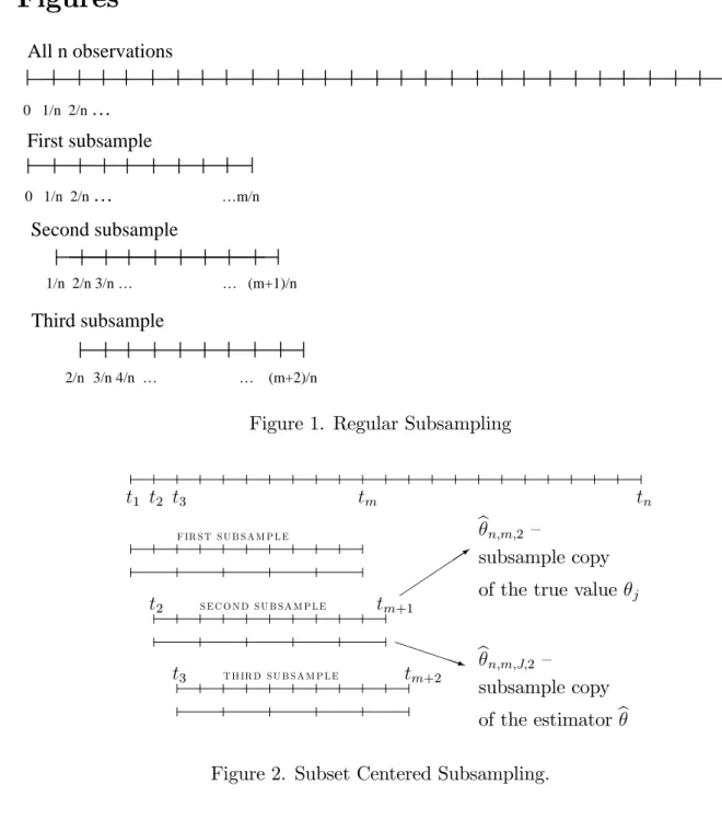
We have 0 < j K; where K is the number of subsamples, K = n m+ 1: See Figure 1 in the appendix for a graphical illustration of the subsamples. In our case where X is only observed at a discrete set of points the data Yj consists of a …nite set of points of lower cardinality than n: The

estimator bn =b(Y) =RVn;when Y consists of all data.

Assumption 5.3.1 of Politis, Romano and Wolf (1999) is satis…ed, i.e., the sampling distribution of n(bn ) converges weakly. Therefore, in the setting of continuous observations and long-span

asymptotics, the intuition laid out in the introduction applies and V should be approximated by (2), i.e., b Vregular =m 1 K K X j=1 b_n;m;j b_n 2:

4_{Subsampling results have also been developed for heteroscedasticity that vanishes in the limit, i.e., is close to}

homoscedasticity. This is an unrealistic setting in in…ll asymptotics.

5_{We will present the version of regular subsampling that uses overlapping subsamples. All the results hold also}

with non-overlapping subsamples. However, for the cases discussed in Politis, Romano, and Wolf (1999), it achieves higher e¢ ciency.

However, in our setting, it is easy to see that Vb is not a consistent estimator for V. This is due tobn;m;j only estimating a part ofbn and the asymptotic distribution of m(bn;m;j ) diverging to

in…nity instead of being the same as that of n(bn ). As a result, we have

Proposition 1. Let m_{! 1} and m=n_!0 as n _{! 1}: We have

E Vbregular =m 2 +o(m):

4

In…ll price subsampling

In this and the next section we consider two subsampling schemes that are motivated by the literature on estimating QV in the presence of measurement error. Both recover the principle that m(bn;m;j )

has the same asymptotic distribution as n(bn ).

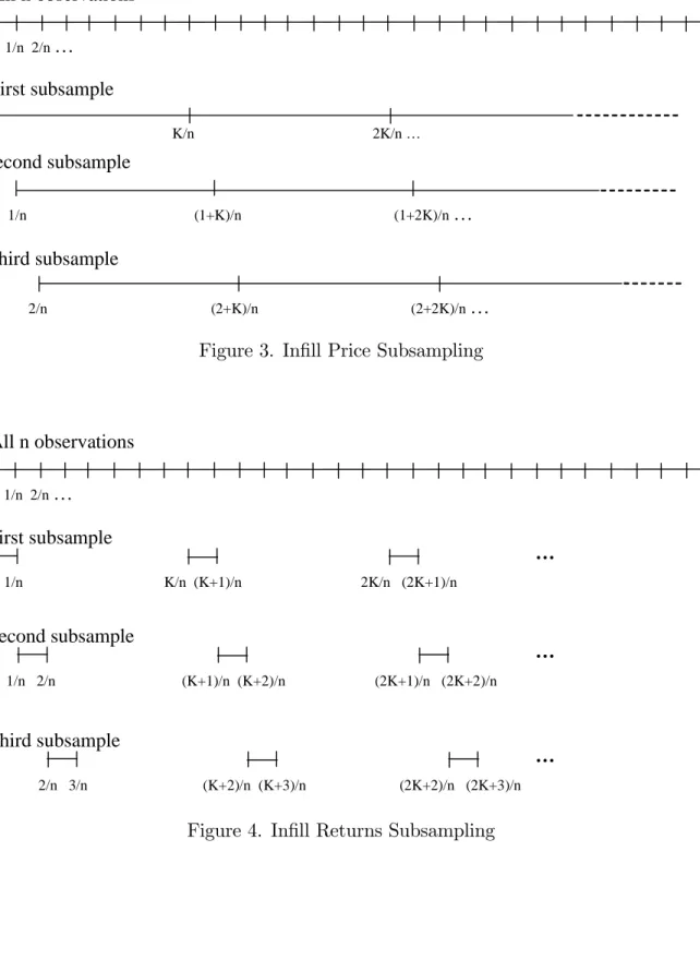
First, we explore a subsampling scheme that exactly mirrors the construction of subsamples in the estimator of QVX of Zhang, Mykland, and Aït-Sahalia (2005). Let the subsamples consist of

data that are K observations apart. In particular, write K (m+ 1) = n and construct the jth

subsample Yj and the estimator of on this subsample as follows (see Figure 3 in the appendix for

a graphical illustration),

Ej;m =fts:s =j+i(K+ 1); i= 1; : : : ; mg; Yj =fX(t) :t2Ej;mg;

b_n;m;j =b(Yj):

In each subsample we have m+ 1 (log-)prices and hence m returns. For j = 1; : : : ; K

b_n;m;j = X t2Ej;m (Xt Xt; ) 2 = m X i=1 Xtj+iK Xtj+(i 1)K 2 ;

where Xt; denotes the preceding element to Xt whereXt2 Ej;m;h.

We can easily see that m(bn;m;j )has the same asymptotic distribution as n(bn ). Therefore,

we consider the estimator of V = 2IQas in (2),

b VIn…ll price =m 1 K K X j=1 bn;m;j bn 2 :

Proposition 2. Let m_{! 1} and m=n_!0 as n _{! 1}: We have

E VIn…ll priceb _!EV; Var VIn…ll priceb =O(1): (6) This estimator is asymptotically unbiased, but it never converges in probability to the true V. Why do we have this problem? Note that any two subsamples fully overlap (in terms of time covered by variances involved; see Figure 3), apart from end e¤ects. As a result, the asymptotic correlation between estimators on any two subsamples is one. We have

Cov b2_n;m;i;b2_n;m;j Var b2_n;m;i =O m 2 ;

and so the failure of consistency follows. We next consider a modi…cation that is motivated by this problem. In the following section we construct subsamples that do not overlap at all while preserving the property that m(bn;m;j )has the same asymptotic (conditional) variance as n(bn ):

5

In…ll Returns Subsampling

To avoid the problem of in…ll price subsampling, consider subsampling one-period returns rti =

Xti Xti 1 instead of log-pricesXt. See Figure 4 in the appendix for a graphical illustration.

Let the subsamples consist of returns that are K observations apart. In particular, write K

(m+ 1) =n and construct thejth _{subsample Y}

j and the estimator of on this subsample as follows,

Ej;m =fts:s =j+i(K+ 1); i= 1; : : : ; mg Yj =fr(t) :t2Ej;mg:

In each subsample we have m returns. For j = 1; : : : ; K

b_n;m;j =K X t2Ej;m r2_t =K m X i=1 r2_t j+(i 1)K =K m X i=1 Xtj+(i 1)K Xtj+(i 1)K 1 2 :

De…nebn as before and b VIn…ll returns =m 1 K K X j=1 b_n;m;j b_n 2: (7)

As opposed to the previous formulation, we now have Cov(bn;m;i;bn;m;j) = 0 for i 6=j;6 which leads

us to

Proposition 3. Let m _{! 1} and m=n _! 0 as n _{! 1}: Assume that volatility paths are a.s.

Hölder continuous of order larger than 1/2. We have

b

VIn…ll returns p

!V: (8)

Without imposing some smoothness on the volatility path VbIn…ll returns is biased due to the large

gaps we have in the subsamples (see Figure 3). For asymptotic unbiasedness of VbIn…ll returns, we need

the expected value of the estimator on each subsample to converge to su¢ ciently fast. If volatility path is càdlàg, we have, conditional on _f tg,

Ebn;m;j =K m X i=1 Z [j+(i 1)K]=n [j+(i 1)K 1]=n 2 (u)du _! Z 1 0 2 (u)du=

due to Riemann integrability of sample paths of_f t; t2[0;1]g. However, what we need for asymptotic

unbiasedness of VbIn…ll returns, is E(bn;m;j) = o(m 1=2). This is because of the scaling factor min

(7), which appears because we are estimating the asymptotic (conditional) variance.

Finally, we consider constructing an estimator ofV that similarly builds on the principle of regular subsampling, but uses a di¤erent centering.

6

Subset Centered In…ll Subsampling

In regular subsampling, the problem was that we were centering our sample variance at "the wrong quantity". In the formula for Vbregular;

b Vregular =m 1 K K X j=1 b_n;m;j b_n 2;

the quantitybnplays the role of , but the problem is thatbn;m;j 9 and soVbregular explodes. In the

two previous sections we rede…ned bn;m;j so as to recover the principlebn;m;j ! and saw this does

not work very well. Instead, consider centering estimators at j such that bn;m;j ! j and then use 6_{This covariance is exactly zero if the drift is zero. It is negligible is the drift is non-zero.}

the property of integrated variance that it can be added up over subsamples to recover the integrated variance over the full sample, P_j j = . Now, j is not observable and the best proxy for j we

have is realised volatility over the subsample, bn;m;j. Therefore, we have to use something else to

play the role of the estimator. So de…ne bn;m;J;j to be realised volatility calculated using every Jth

observation of thejth_{subsample of lengthm (J << m), see Figure 2 in the Appendix for a graphical}

illustration. Since it has a slower rate of convergence thanbn;m;j, the error of usingbn;m;j instead of

is negligible. Our estimator of V becomes

b VSC = n2 mKJ K X k=1 bn;m;J;k bn;m;k 2 :

Here, the number of subsamplesK depends on how much di¤erent subsamples overlap. Increasing the amount of overlap does not change the rate of convergence ofVb, but it decreases the asymptotic (conditional) variance, so maximum overlap estimator is preferred. See the Monte Carlo simulations (Figure 5e) for an illustration.

Proposition 4. Let m_{! 1},J _{! 1}, m=n_!0, and J=m_!0 as n _{! 1}: We have

b

VSC p

!V: (9)

The estimator is similar in structure to Lahiri, Kaiser, Cressie, and Hsu (1999). They similarly use two grids for subsampling to predict stochastic cumulative distribution function. However, they assume that the underlying process is stationary and their asymptotic framework is mixed in…ll and increasing domain.

7

Numerical Work

In this section we examine the numerical properties of our estimators of V plus several benchmarks. In our experience the performance of the corresponding con…dence intervals here is closely matched by the performance of the estimated variance. In Section 7.1 we simulate the Heston (1993) model with continuous price sample paths. In Section 7.2. we allow price paths to exhibit jumps.

7.1

Continuous prince paths

We do a simulation comparison of the above subsampling methods, plus realized quarticity. We simulate the Heston (1993) model:

dXt = ( t vt=2)dt+ tdBt dvt = ( vt)dt+ v

1=2 t dWt;

where vt= 2t, and Bt; Wt are independent standard Brownian motions.

We take parameters from Zhang, Mykland, and Aït-Sahalia (2005): = 0:05; = 5; = 0:04;

= 0:5: We set the length of the sample path to 22500, which is a proxy for 23400 that is the number of seconds in a business day. We set the time between observations corresponding to one second when a year is one unit, and the number of replications to be 100,000. For Vbregular;VbIn…ll price;

b

VIn…ll returns; and VbSC; we use m = pn: For VbSC we use J = 15: We hold the volatility sample path

constant across simulations for easier comparison. Appendix contains Figure 5 showing the results.

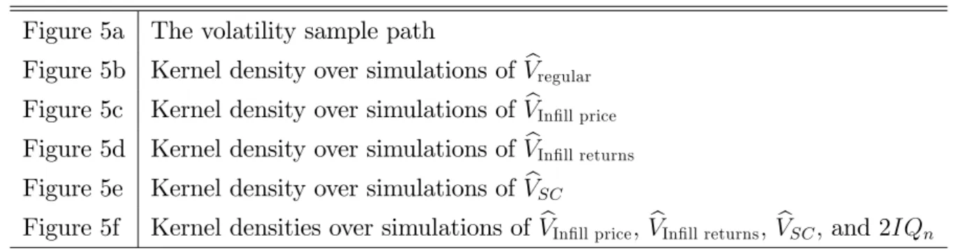
Table 1. Finite sample distributions of di¤erent methods Figure 5a The volatility sample path

Figure 5b Kernel density over simulations of Vbregular

Figure 5c Kernel density over simulations of VbIn…ll price

Figure 5d Kernel density over simulations of VIn…ll returnsb

Figure 5e Kernel density over simulations of VbSC

Figure 5f Kernel densities over simulations of VbIn…ll price;VbIn…ll returns; VbSC; and 2IQn

From the simulated volatility sample path (Figure 5a) we can approximate the trueV ar(RV) =

V = 2IQ and we get 4:05 10 6. Also, this can be approximated by the (scaled) sample variance of RV over simulations. Here is a brief summary comparing the means of feasible methods with infeasible benchmarks:

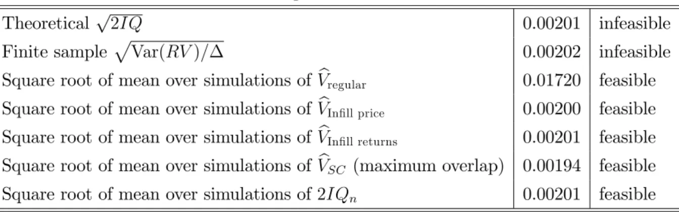
Table 2. Finite sample means of di¤erent methods

Theoreticalp2IQ 0.00201 infeasible Finite sample pVar(RV)= 0.00202 infeasible Square root of mean over simulations ofVbregular 0.01720 feasible

Square root of mean over simulations ofVIn…ll priceb 0.00200 feasible Square root of mean over simulations ofVbIn…ll returns 0.00201 feasible

Square root of mean over simulations ofVbSC (maximum overlap) 0.00194 feasible

Square root of mean over simulations of2IQn 0.00201 feasible

We see that Vbregular overestimates the true V by a large factor, thus supporting the asymptotic

result. The other feasible methods work well. We can also see that VbIn…ll price is asymptotically

unbiased, whereas from Figure 5c in the appendix we see that its distribution over simulations is strongly right-skewed. From Figure 5f we can see that 2IQn has the smallest variance, re‡ecting the

fact that is has much faster rate of convergence. Our proposed estimator VbSC has some …nite sample

negative bias. One could do a …nite sample correction and use _JJ₁VbSC (recallJ = 15, so this factor

is non-negligible), see section A.4.2. for theoretical justi…cation. Adjusted estimator _JJ₁VbSC has a

smaller negative bias in simulations.

One of the parameters to choose in our proposed estimatorVbSC is the amount of overlap between

di¤erent subsamples, which a¤ects the total number of subsamplesK:We do a simulation exercise to see how exactly it a¤ects the …nite sample properties. Figure 5e shows the …nite sample distribution for three di¤erent scenarios, no overlap, maximum overlap and an intermediate case. We know from theory that the amount of overlap does not a¤ect the convergence rate. The simulations, however, indicate that it decreases the asymptotic conditional variance, i.e., VbSC with the maximum amount

of overlap (with K =n m+ 1) gives the lowest variance. This phenomenon is also observed in the long span asymptotic framework.

7.2

Jumps

Now we consider the case of possibly discontinuous sample paths. In this case, the realised volatility again converges to the quadratic variation. However, quadratic variation does not coincide with integrated volatility, but instead, it is equal to integrated volatility plus the sum of squared jumps,

where Xt is the left limit ofXt,

Xt = lim

s"t Xs:

We have that Xt =Xtif there are no jumps at time t. The asymptotic distribution ofRV is mixed

normal with asymptotic (conditional) variance

V = 2IQ+ 4X(Xt Xt )2 2t. (10)

It is well known that realised quarticity is inconsistent for V;Barndor¤-Nielsen and Shephard (2006). There are two available consistent estimators of V under the scenario of jumps. One is Aït-Sahalia and Jacod (2005), which uses truncated power variations. The second is that of Veraart (2007) who obtains an estimator forV as a linear combination of known estimators ofIQand generalized bipower variation. This estimator entails estimation of 2t for eacht in [0,1] using a histogram approach. In

this section we will consider all estimators of section 7.1 plus Veraart’s estimator.

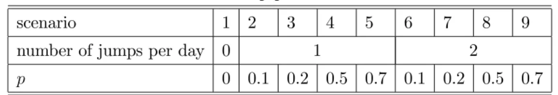
The continuous part of the price paths are simulated as in Heston (1993), where every simulation has its own volatility path. We then add jumps as follows. We consider nine scenarios with none, one, or two jumps per day, with jump times that are uniformly distributed over the day with di¤erent jump size distributions (as in, for example, Barndor¤-Nielsen and Shephard (2006)). We consider four di¤erent sizes of the jumps, governed by a parameter p. In particular, we draw the the size of the jump from a normal p.d.f. with variance p times the integrated volatility, N(0; pIV). This is the setup for jumps considered by Huang and Tauchen (2005) and Veraart (2007).

Table 3. Jump parameterization

scenario 1 2 3 4 5 6 7 8 9 number of jumps per day 0 1 2

p 0 0.1 0.2 0.5 0.7 0.1 0.2 0.5 0.7

We report the results by graphing the kernel densities of the studentised RV by the infeasible

QV and respective estimator of V, as follows

t =pn RV_p QV

b

V

!

:

Ideally, these kernel densities should coincide with the p.d.f of a standard normal distribution, which we superimpose on the estimated density oft. Figures (6) to (11) contain the results. Nine sub-plots

in each graph represent 9 scenarios as in Table 3. Note that scenario 1 is very similar to the setup of section 7.1, but now we use a di¤erent way of representing results (because there is no one true

V anymore, it changes across simulations).

After inspecting Figures (6) to (11) we can make several observations. First, from Figures 6 and

10, VbSC and VbVeraart seem to be good estimators ofV in all scenarios. Most probably, this indicates

that VbSC _{preserves consistency even in this richer context. This seems reasonable, because} b n;m;J;k

and bn;m;k both converge to the same quantity, i.e., quadratic variation over the (little) time interval

they cover.

Second, from Figure 7, we see thatVbin…ll returns estimator, which was consistent for the variance of RV in the case of no jumps, is not consistent anymore. The intuition for this failure is straightforward. Although bn converges to quadratic variation, its subsampled version bn;m;j does not, hence the

estimator Vbin…ll returns overestimatesV by a large factor (hence the peaks at zero of estimated density

of tIn…ll returns). This intuition is the same as for the failure of consistency ofVregularb in the case of no jumps (see Section 3).

Third, from Figure 8 we see that the performance of Vbin…ll price is not worsened by adding jumps.

The intuition is that Vbin…ll price does not su¤er from the problem ofVbin…ll returns. In Vbin…ll price, bothbn

andbn;m;j pick up the same jumps and converge to the same quantity. Therefore, the estimator most

probably remains asymptotically unbiased, though retains the problem of high correlation between subsamples and hence is inconsistent. Although a direct comparison between Figures (5c) and (8) should be avoided since the latter does not hold volatility path constant across simulations, we can see that the large mass below the true quantity V in Figure (5c) is re‡ected in heavy tails of kernel density in all nine scenarios of (8).

Fourth, from Figure 9, we see that2IQn estimatesV well when there are no jumps, but is clearly

not consistent for V when jumps are present.

8

Conclusions and Extensions

In this paper we have investigated the use of subsampling for conducting inference about quadratic variation. We have established two negative results. First, the usual subsampling method as in Poli-tis, Romano, and Wolf (1994) is inconsistent. Second, the subsampling method of Zhang, Mykland, and Aït-Sahalia (2005) is also inconsistent. We have also proposed two alternative subsampling

meth-ods and established their consistency under weak assumptions (given the basic framework we have adopted). The simulation experiments con…rm that our methods can be consistent in the presence of leverage and in the presence of jumps.

There is much further work that can be done. Our method can also be applied to other estimators like bipower variation, Barndor¤-Nielsen and Shephard (2006) and the leverage estimator of Mykland and Zhang (2007). It is important to generalize the process that X can follow. For example, one could allow for leverage and jumps. Our simulations show that this can be done to conduct consistent inference for quadratic variation. Inference for integrated volatility would involve subsampling of tripower quarticity or other consistent estimators of integrated volatility. Also, one could allow for measurement error that contaminates X, in which case one has to consider subsampling T SRV or realized kernels instead of RV as estimators for QVX. Examples of cases where only the asymptotic

theory has been developed, but not the tools for inference, include estimation of quadratic variation with autocorrelated measurement error (Aït-Sahalia, Mykland, and Zhang 2006a) or with endogenous measurement error (Kalnina and Linton 2006).

A

Appendix

Recall that we are assuming no leverage, so that we can condition on the volatility path. Also, all arguments are done for a zero drift. Extension to nonzero drift is straightforward (given that we assume a locally bounded drift, and hence bounded drift w.l.o.g. for the purposes of consistency). In the proofs of proposition 3 and 4 we use the following result, which is a modi…cation of Linton (2000, Lemma 1).

Lemma 0. Let ( n; ) be a sequence of random variables with n scalar and =f t; t 2[0;1]g:

Suppose that E( nj ) = mn( ) and Var( nj ) = vn( ) almost surely, where mn( ); vn( )

p

! 0:

Then, n

p

!0:

A.1

Proof of Proposition 1

The jth _{subsample contains observations}

fXj 1; Xj; : : : ; Xm+j 1g. Then b(Yj) = m X i=1 (Xj+i 1 Xj+i 2)2:

In this case, the number of subsamples is K = n m+ 1: Let zj;i =

R((j+i 1)=n

(j+i 2)=n udWu and yj;i =

(R_(j+i((j+i_2)=n1)=n udWu)2 2j;i; which are independent (across i for given j) and mean zero random

variables conditional on the process 2u; where

2 j;i= E[( Z ((j+i 1)=n (j+i 2)=n udWu)2] = Z ((j+i 1)=n (j+i 2)=n 2 udu=O(1=n):

In above we use use local boundedness of 2

u (which follows from the assumption that paths of are

càdlàg) to conclude orders of magnitude, i.e.,

Z ((j+i 1)=n (j+i 2)=n 2 udu 1 nsupu 2 u =O(1=n):

We use this argument of boundedness to conclude stochastic orders of magnitude throughout the appendix. We have var (zj;i) = E 2 4 Z ((j+i 1)=n (j+i 2)=n udWu !23 5= 2_j;i var (yj;i) = E 2 4 Z ((j+i 1)=n (j+i 2)=n udWu !43 5 E2 2 4 Z ((j+i 1)=n (j+i 2)=n udWu !23 5 = 3 Z ((j+i 1)=n (j+i 2)=n 2 udu !2 Z ((j+i 1)=n (j+i 2)=n 2 udu !2 = O(1=n2):

We show the following lemmas.

Lemma 1.1. As n_{! 1} E " _K X j=1 bn;m;j # =m Z 1 0 2 udu+O m2 n : Lemma 1.2. As n_{! 1} K X j=1 E b2_n;m;j =O m 2 n :

Then, b V = m 1 K K X j=1 b_n;m;j b_n 2 = m K K X j=1 b_n;m;j 2+ bn 2 + 2 bn;m;j bn = m K K X j=1 b_n;m;j 2+Op m1=2n 1=2 = m K K X j=1 b2_n;m;j +m 2 2m 1 K K X j=1 bn;m;j+op(1) and E(Vb) = m K K X j=1 E(b2_n;m;j) +m 2 2m 1 K K X j=1 E(bn;m;j) +o(1) = m KO m2 n +m 2 _2m 1 K m Z 1 0 2 udu+O m2 n +o(1) = m 2+o(m)_{! 1}; using K =n m+ 1 and m2=n=o(1):

Proof of Lemma 1.1. We have

E " _K X j=1 b_n;m;j # = K X j=1 m X i=1 E z_j;i2 = K X j=1 m X i=1 Z ((j+i 1)=n (j+i 2)=n 2 udu = K X j=1 Z (m+j 1)=n (j 1)=n 2 udu = m Z 1 0 2 udu+O m2 n :

Proof of Lemma 1.2. We have K X j=1 E b2_n;m;j = K X j=1 E 2 4 m X i=1 z_j;i2 !23 5 = K X j=1 E 2 4 m X i=1 ( 2_j;i+yj;i) !23 5 = K X j=1 m X i=1 Ey_j;i2 + K X j=1 m X i=1 m X i0₌₁ 2 j;i 2 j;i = 2 K X j=1 m X i=1 Z ((j+i 1)=n (j+i 2)=n 2 udu !2 + K X j=1 m X i=1 m X i0=1 2 j;i 2 j;i = O m 2 n :

A.2

Proof of Proposition 2

A.2.1 Notation and preliminary calculations

Let zj;i = Z (j+iK)=n (j+(i 1)K)=n udWu; and so b_n;K;j = m X i=1 z2_j;i;

where: z_j;i2 = 2_j;i+yj;i; 2j;i =E[(

R(j+iK)=n (j+(i 1)K)=n udWu) 2_{] =}R(j+iK)=n (j+(i 1)K)=n 2 udu;and yj;i = ( R(j+iK)=n (j+(i 1)K)=n udWu) 2 2

j;i; which are independent (across i for given j) and mean zero

random variables conditional on the process 2

u:That is, E[zj;izj;i0] =E[yj;iyj;i0] = 0 whenever i6=i0:

Furthermore, zj;i is conditionally normal and so satis…esE[zj;i4 ] = 3E2[zj;i2 ]: Note that, forj < j0,

E[zj;izj0_;i0] = 8 > > < > > : R(minfj;j0_g+iK)=n (maxfj;j0_g+(i 1)K)=n 2 udu 6= 0 i=i0 R(j0_+i0_K)=n (j+i0K)=n 2 udu6= 0 i=i0+ 1 0 _ji i0_{j>1; i=i}0 _1:

Furthermore, E[yj;izj;i] = 0; and var (zj;i) =E 2 4 Z (j+iK)=n (j+(i 1)K)=n udWu !23 5= 2_j;i = Z (j+iK)=n (j+(i 1)K)=n 2 udu =Op(K=n) var (yj;i) = E 2 4 Z (j+iK)=n (j+(i 1)K)=n udWu !43 5 E2 2 4 Z (j+iK)=n (j+(i 1)K)=n udWu !23 5 = 2 Z (j+iK)=n (j+(i 1)K)=n 2 udu !2 = 2K n Z (j+iK)=n (j+(i 1)K)=n 4 udu+op K2=n2 =Op(K2=n2); since _Z (j+iK)=n (j+(i 1)K)=n 2 udu !2 = K n Z (j+iK)=n (j+(i 1)K)=n 4 udu+o(K 2_=n2_{): (11)}

We prove this result below.

By adding these results over all subsamples, we get that for each j and each j0_,

Cov(bn;m;j;bn;m;j0) =O m 1 : (12)

Proof of (11).This is established as follows. Suppose thatf is a bounded positive continuous

function on [0;1]; say. Then for >0; g( ) = R₀ f(x)dx is of order as _!0; because

Z 0

f(x)dx sup

x2[0;] f(x):

Furthermore, g is di¤erentiable in with g0_{( ) =f( ): Therefore, by the mean value theoremg( ) =}

g(0) + g0_{( ) = f( ) for some : Therefore,}

Z 0

f(x)dx 2

= 2f2( ):

Furthermore, f2 _{is also a bounded continuous function on[0;1] and satis…es} Z

0

f2(x)dx sup

x2[0;] f2(x)

Z 0

f2(x)dx= f2( )

for some : By continuity of f2 _{at 0;}

lim

#0

f2_{( )} f2_{( )} = 1;

and it follows that _Z

0 f(x)dx 2 = Z 0 f2(x)dx+o( 2):

A.2.2 Main proof

Write b V = m K K X j=1 b2_n;m;j +mb2_n 2mbn 1 K K X j=1 b_n;m;j = m K K X j=1 b2_n;m;j +m 2 2m 1 K K X j=1 b_n;m;j+op(1);

where the approximation is valid by Barndor¤-Nielsen and Shephard (2002). We make use of the following lemmas.

Lemma 2.1. E " 1 K K X j=1 b_n;m;j # = 1 K K X j=1 Z 1 K=n+j=n j=n 2 udu: Lemma 2.2. E " 1 K K X j=1 b2 n;m;j # = 2 n K X j=1 Z 1 j=n j=n 4 udu+ 1 K K X j=1 Z 1 K=n+j=n j=n 2 udu !2 +o 1 m : Lemma 2.3. Var m K K X j=1 b2_n;m;j 2m 1 K K X j=1 b_n;m;j ! =O(1):

These lemmas imply that EVb = m K K X j=1 E[b2_n;m;j] +m 2 2m 1 K K X j=1 E[bn;m;j] +o(1) = 2m n K X j=1 Z 1 K=n+j=n j=n 4 udu+ m K K X j=1 Z 1 K=n+j=n j=n 2 udu !2 +m Z 1 0 2 udu 2 2m Z 1 0 2 udu 1 K K X j=1 Z 1 K=n+j=n j=n 2 udu+o(1):

We have to show that

R = Z 1 0 2 udu 2 + 1 K K X j=1 8 < : Z 1 K=n+j=n j=n 2 udu !2 2 Z 1 0 2 udu Z 1 K=n+j=n j=n 2 udu 9 = ;=o(K=n): (13) This is true because, write I = R₀1 2

udu; Ij=n = Rj=n 0 2 udu; and I1 K=n+j=n = R1 1 K=n+j=n 2 udu: Then R = I2+ 1 K K X j=1 I2 2I(Ij=n+I1 K=n+j=n) + (Ij=n+I1 K=n+j=n)2 2I(I (Ij=n+I1 K=n+j=n)) = 1 K K X j=1 (Ij=n+I1 K=n+j=n)2 =O(K2=n2): Therefore, EVb = 2m n K X j=1 Z 1 K=n+j=n j=n 4 udu+o(1) = 2m n K X j=1 Z 1 0 4 udu+o(1) = 2 Z 1 0 4 udu+o(1);

Proof of Lemma 2.1. We have E " 1 K K X j=1 b_n;m;j # = 1 K K X j=1 m X i=1 E z_j;i2 = 1 K K X j=1 m X i=1 Z (j+iK)=n (j+(i 1)K)=n 2 udu = 1 K K X j=1 Z 1 K=n+j=n j=n 2 udu:

Proof of Lemma 2.2. We have

1 K K X j=1 E b2_n;m;j = 1 K K X j=1 E 2 4 m X i=1 z2_j;i !23 5 = 1 K K X j=1 E 2 4 m X i=1 ( 2_j;i+yj;i) !23 5 = 1 K K X j=1 m X i=1 Ey_j;i2 + 1 K K X j=1 m X i=1 m X i0=1 2 j;i 2 j;i0 = 2 n K X j=1 m X i=1 Z (j+iK)=n (j+(i 1)K)=n 2 udu !2 + 1 K K X j=1 Z 1 j=n j=n 2 udu !2 = 2 n K X j=1 Z 1 K=n+j=n j=n 4 udu+ 1 K K X j=1 Z 1 K=n+j=n j=n 2 udu !2 +o 1 m : by (11).

Proof of Lemma 2.3. This can be seen from the covariance betweenbn;K;j and bn;K;i:

A.3

Proof of Proposition 3

Ebn;m;j = KE m X i=1 Xj+(i 1)K Xj+(i 1)K 1 2 = K m X i=1 Z (j+(i 1)K)=n (j+(i 1)K 1)=n 2 udu = Z 1 0 2 udu+o(1)

by Riemann integrability of 2u: Furthermore,

Varbn;m;j = K2Var m X i=1 Xj+(i 1)K Xj+(i 1)K 1 2 = K2 m X i=1

Var Xj+(i 1)K Xj+(i 1)K 1

2 = 2K2 m X i=1 Z (j+(i 1)K)=n (j+(i 1)K 1)=n 2 udu !2 = 2 m Z 1 0 4 udu+o 1 m :

Now we calculate the expected value of the estimator.

EVbIn…ll returns = Em 1 K K X j=1 b_n;m;j b_n 2 = m K K X j=1 E bn;m;j Ebn;m;j 2 +R = 2 Z 1 0 4 udu+o(1) +R; where R = m K K X j=1 En bn;m;j Ebn;m;j Ebn;m;j bn o + m K K X j=1 E Ebn;m;j bn 2 = m K K X j=1 EnOp m 1=2 Ebn;m;j bn o + m K K X j=1 E Ebn;m;j bn 2 :

We know that bn = O n 1=2 : Therefore, have R = o(1) if Ebn;m;j = op m 1=2 : For

this, Riemann integrability is not enough, which is why we have assumed Hölder continuity of order larger than 1=2.

Now we calculate the variance of VbIn…ll returns. To facilitate calculations, introduce the usual

notation: zj;i= Z (j+(i 1)K)=n (j+(i 1)K 1)=n udWu b_n;m;j =K m X i=1 z_j;i2

z_j;i2 = 2_j;i+yj;i

2 j;i = E[( Z (j+(i 1)K)=n (j+(i 1)K 1)=n udWu)2] = Z (j+(i 1)K)=n (j+(i 1)K 1)=n 2 udu yj;i = ( Z (j+(i 1)K)=n (j+(i 1)K 1)=n udWu)2 2j;i:

We …rst do some preliminary calculations.

Eyj;i = 0; so thatVar (yj;i) = Ey2j;i

Ey_j;i2 = E 8 < : Z (j+(i 1)K)=n (j+(i 1)K 1)=n udWu !2 2 j;i 9 = ; 2 = E 8 < : Z (j+(i 1)K)=n (j+(i 1)K 1)=n udWu !4 + 2_j;i 2 2 Z (j+(i 1)K)=n (j+(i 1)K 1)=n udWu !2 2 j;i 9 = ;

Ey_j;i4 = E 8 < : Z (j+(i 1)K)=n (j+(i 1)K 1)=n udWu !2 2 j;i 9 = ; 4 = E 8 < : Z (j+(i 1)K)=n (j+(i 1)K 1)=n udWu !8 + 2_j;i 4 4 Z (j+(i 1)K)=n (j+(i 1)K 1)=n udWu !2 2 j;i 3 4 Z (j+(i 1)K)=n (j+(i 1)K 1)=n udWu !6 2 j;i + 6 Z (j+(i 1)K)=n (j+(i 1)K 1)=n udWu !4 2 j;i 2 9 = ;

= 105 2_j;i 4+ 2_j;i 4 4 2_j;i 2_j;i 3 4 15 2_j;i 3 2_j;i + 6 3 2_j;i 2 2_j;i 2

= 2_j;i 4_f105 + 1 4 60 + 18_g= 60 2_j;i 4:

Using the same approximation of VbIn…ll returns as in Proposition 1, the variance of VbIn…ll returns

becomes

VarVbIn…ll returns = Var

" m K K X j=1 bn;m;j 2 +op(1) # = m 2 K2 K X j=1 Var bn;m;j 2 +o(1):

To show VarVIn…ll returnsb = o(1); we show that Var bn;m;j 2

= Var b2_n;m;j 2bn;m;j =

o(Km 2). In order to do that, we proceed in three steps. That is to say, to calculate Var(x), we …rst …rst calculate E(x), theny=x E(x), and …nally E(y2_):

Step 1. We have E b2_n;m;j 2bn;m;j = E 2 4 ( K m X i=1 2 j;i+yj;i )2 2 K m X i=1 2 j;i+yj;i 3 5 = E 8 < :K 2 m X i=1 2 j;i !2 +K2 m X i=1 yj;i !2 + 2K2 m X i=1 2 j;i m X i=1 yj;i 9 = ; 2 K m X i=1 2 j;i

= K2 m X i=1 2 j;i !2 +K2 m X i=1 Ey2_j;i 2 K m X i=1 2 j;i = K2 m X i=1 2 j;i !2 + 2K2 m X i=1 2 j;i 2 2 K m X i=1 2 j;i: Step 2. We have b2_n;m;j 2bn;m;j E b 2 n;m;j 2bn;m;j = ( K2 m X i=1 2 j;i+yj;i )2 2 K m X i=1 2 j;i+yj;i E b 2 n;m;j 2bn;m;j = K2 m X i=1 2 j;i !2 +K2 m X i=1 yj;i !2 + 2K2 m X i=1 2 j;i m X i=1 yj;i 2 K m X i=1 2 j;i 2 K m X i=1 yj;i K2 m X i=1 2 j;i !2 2K2 m X i=1 2 j;i 2 + 2 K m X i=1 2 j;i = K2 m X i=1 yj;i !2 + 2K2 m X i=1 2 j;i m X i=1 yj;i 2 K m X i=1 yj;i 2K2 m X i=1 2 j;i 2 = K2 m X i=1 yj;i !2 2K2 m X i=1 2 j;i 2 + 2K m X i=1 yj;i K m X i=1 2 j;i ! = K2 m X i=1 yj;i !2 2K2 m X i=1 2 j;i 2 +op n 1 ;

because even without any smoothness assumptions on we have KPm_i=1 2

j;i = o(1) and KPm_i=1yj;i =O(Kmn 2) =O(n 1):

n 1_{), is} E 2 4K2 m X i=1 yj;i !2 2K2 m X i=1 2 j;i 2 3 5 2 = K4 2 4E m X i=1 yj;i !4 + 4E m X i=1 2 j;i 2 !2 4 m X i=1 2 j;i 2 E m X i=1 yj;i !23 5 = K4 2 4E m X i=1 yj;i !4 + 4 m X i=1 2 j;i 2 !2 8 m X i=1 2 j;i 2 !23 5 = K4 2 4E m X i=1 yj;i !4 4 m X i=1 2 j;i 2 !23 5 = K4 2 4 m X i=1 Ey_j;i4 + 3 m X i0=1;i0₆=i m X i=1 Ey_j;i2 Ey2_j;i 4 m X i=1 2 j;i 2 !23 5 = K4 2 460 m X i=1 2 j;i 4 + 12 m X i0=1;i0₆=i m X i=1 2 j;i 2 ₂ j;i0 2 4 m X i=1 2 j;i 2 !23 5 = K4 " 56 m X i=1 2 j;i 4 + 8 m X i0=1;i0₆=i m X i=1 2 j;i 2 ₂ j;i0 2 # = O K4mn 4 +O K4m2n 4 =O m 2 =o(Km 2):

This implies VarVb _!0and so we have mean square convergence and so (8) follows by Chebyshev’s inequality.

A.4

Proof of Proposition 4

In the …rst subsection of this proof we explain the notation, in the second we show that the bias of

b

VSC is negligible, i.e.,E(VbSC) V =o(1), and in the third subsection we show thatVar(VbSC) =o(1),

A.4.1 Notation for VbSC

Much of the notation is the same as for the other estimators. K is the number of subsamples. m

is the number of high frequency returns in of each subsample. J is the number of high frequency returns that ‘…t into’one low frequency return (see Figure 2 for a graphical illustration),1< J < m. There are m=J number of low frequency in each subsample. Takem ... J (i.e., m divisible by J).

The proof is for a general amount of overlap between subsamples, so introduce a variable s, for ‘shift’. If subsamples are constructed as observations in a window, we move the window by s=n

to get every next subsample. For example, s = m corresponds to no overlap between subsamples and s = 1 corresponds to maximum possible overlap. Assume m ... s. As we show below, we have

K =n=s m=s+ 1.

The ‘subsample copies’of the RV estimator (bn;m;j in (2)) will be

b_n;m;J;1 = m=J_P i=1 XJ i XJ(i 1) 2 ; bn;m;J;2 = m=J_P i=1 XJ i+s XJ(i 1)+s 2 ; etc:;

so that the copy corresponding to the kth _{subsample is}

b_n;m;J;k = m=J_P i=1 XJ i+s(k 1) XJ(i 1)+s(k 1) 2 :

The number of subsamples is the k such that

Jm J +s(kmax 1) =n )kmax K =n=s m=s+ 1: We have Ebn;m;J;k = m=J_P i=1 Z [J i+s(k 1)]=n [J(i 1)+s(k 1)]=n 2 udu= Z [m+s(k 1)]=n s(k 1)=n 2 udu:

The ‘subsample copies’of the true parameterQV ( in (2), except that we have a di¤erent ‘copy’ for each subsample for our centering) will be

b_n;m;1 = m P i=1 (Xi Xi 1)2; bn;m;2 = m P i=1 (Xi+s Xi 1+s)2; etc: b_n;m;k = m P i=1 Xi+s(k 1) Xi 1+s(k 1) 2 : We have Ebn;m;k = m P i=1 Z [i+s(k 1)]=n [i 1+s(k 1)]=n 2 udu= Z [m+s(k 1)]=n s(k 1)=n 2 udu:

Recall that the estimator ofV is b VSC = n2 mKJ K X k=1 bn;m;J;k bn;m;k 2 : A.4.2 Derivation of E(VbSC)

Introduce the following notation,

E bn;m;J;k bn;m;k 2 = Eb2_n;m;J;k+ Eb2_n;m;k 2Ebn;m;J;kbn;m;k = Ak+Bk 2Ck; so that we have EVbSC = n 2 mKJ PK k=1(Ak+Bk 2Ck):Then, Ak = Eb 2 n;m;J;k= E " m=J_P i=1 XJ i+s(k 1) XJ(i 1)+s(k 1) 2 #2 = m=J_P i=1 E XJ i+s(k 1) XJ(i 1)+s(k 1) 4 +2P i0>i m=J_P i=1 E XJ i+s(k 1) XJ(i 1)+s(k 1) 2 E XJ i0+s(k 1) XJ(i0 1)+s(k 1) 2 = 2 m=J_P i=1 Z [J i+s(k 1)]=n [J(i 1)+s(k 1)]=n 2 u !2 + Z [m+s(k 1)]=n s(k 1)=n 2 udu !2 : Similarly, Bk = Eb 2 n;m;k = E m P i=1 Xi+s(k 1) Xi 1+s(k 1) 2 = 2 m P i=1 Z [i+s(k 1)]=n [i 1+s(k 1)]=n 2 u !2 + Z [m+s(k 1)]=n s(k 1)=n 2 udu !2 :

denote as corresponding summation over low frequency returns m=J_P i=1 Ck;i as follows, Ck = Ebn;m;J;kbn;m;k = Cov bn;m;J;k;bn;m;k + Ebn;m;J;kEbn;m;k = Cov m=J_P i=1 XJ i+s(k 1) XJ(i 1)+s(k 1) 2 ; m P i=1 Xi+s(k 1) Xi 1+s(k 1) 2 ! + Ebn;m;J;kEbn;m;k = m=J_P i=1 Ck;i+ Ebn;m;J;kEbn;m;k:

We then notice thatCk;1 is the variance of the realised volatility over the1st low frequency return,

and Ck;1 = Cov XJ+s(k 1) Xs(k 1) 2 ; m P i=1 Xi+s(k 1) Xi 1+s(k 1) 2 = Cov XJ+s(k 1) Xs(k 1) 2 ; J P i=1 Xi+s(k 1) Xi 1+s(k 1) 2 = Cov " J P j=1 Xj+s(k 1) Xj 1+s(k 1) 2 +2 P j0_>j J P j=1 Xj+s(k 1) Xj 1+s(k 1) Xj0_{+s(k 1)} X_j0 _{1+s(k 1)} ; J P i=1 Xi+s(k 1) Xi 1+s(k 1) 2 = Var J P i=1 Xi+s(k 1) Xi 1+s(k 1) 2 = 2 J P i=1 Z [i+s(k 1)]=n [i 1+s(k 1)]=n 2 u !2 :

Similarly with otherC_k;i0 s and so we have

Ck = 2 J P i=1 Z [i+s(k 1)]=n [i 1+s(k 1)]=n 2 u !2 + Ebn;m;J;kEbn;m;k = 2 J P i=1 Z [i+s(k 1)]=n [i 1+s(k 1)]=n 2 u !2 + Z [m+s(k 1)]=n s(k 1)=n 2 udu !2 = Bk:

Therefore, EVbSC = n 2 mKJ K P k=1 E bn;m;J;k bn;m;k 2 = n 2 mKJ K P k=1 (Ak Bk) = n 2 mKJ K P k=1 8 < :2 m=J_P i=1 Z [J i+s(k 1)]=n [J(i 1)+s(k 1)]=n 2 u !2 2 J P i=1 Z [i+s(k 1)]=n [i 1+s(k 1)]=n 2 u !29₌ ; = 2 n 2 mKJ K X k=1 m=J_P i=1 Z [J i+s(k 1)]=n [J(i 1)+s(k 1)]=n 2 u !2 2 n 2 mKJ K X k=1 m P i=1 Z [i+s(k 1)]=n [i 1+s(k 1)]=n 2 u !2 :

We show just below that the …rst term converges toV:Notice that second term is likeJ 1_{V, which}

means that one could do an easy …nite sample bias correction by estimatingV by J

J 1VbSC instead of b

VSC:Note that in our simulation setup we have J = 15, so the adjustment factor is non-negligible.

We deal with summations in the …rst term by re-grouping the terms so that each group ‘covers’ the interval [0;1]apart from end-e¤ects,

K X k=1 m=J_P i=1 Z [J i+s(k 1)]=n [J(i 1)+s(k 1)]=n 2 u !2 = m=s X p=1 (n m)=J_P i=1 Z J i=n+s(p 1)=n J(i 1)=n+s(p 1)=n 2 u !2 = m=s X p=1 J n Z 1 0 2 udu+o J n = mJ sn Z 1 0 2 udu+o mJ sn :

Now we can conclude asymptotic unbiasedness,

EVbSC = 2 n2 mKJ mJ sn Z 1 0 2 udu+o mJ sn +O J 1 = V +o(1)

A.4.3 Derivation of Var(VbSC) VarVbSC = Var " n2 mKJ K X k=1 b_n;m;J;k b_n;m;k 2 # = n 2 mKJ 2_XK k0=1 K X k=1 Cov bn;m;J;k bn;m;k 2 ; bn;m;J;k0 b_n;m;k0 2 n2 mKJ 2 min(K;k+m=s)_X k0=max(1;k m=s) K X k=1 Cov bn;m;J;k bn;m;k 2 ; bn;m;J;k0 bn;m;k0 2 n2 mKJ 2 2m s K X k=1 Var bn;m;J;k bn;m;k 2 ;

where we use the fact that: 1) all these covariances must be nonnegative, 2) for a …xed term k in the …rst summation, only the terms from k m=s tok+m=s terms in the summation over k0 _{give rise}

to nonzero covariances.

Now we calculate the magnitude ofbn;m;J;k bn;m;k,

Varhbn;m;J;k bn;m;k i = Var " m=J_P i=1 XJ i+s(k 1) XJ(i 1)+s(k 1) 2 Pm i=1 Xi+s(k 1) Xi 1+s(k 1) 2 # = Var " m=J_P i=1 XJ i+s(k 1) XJ(i 1)+s(k 1) 2 m=JP i=1 J P j=1 Xj+J(i 1)+s(k 1) Xj 1+J(i 1)+s(k 1) 2 # = Var m=J_P i=1 " XJ i+s(k 1) XJ(i 1)+s(k 1) 2 PJ j=1 Xj+J(i 1)+s(k 1) Xj 1+J(i 1)+s(k 1) 2 # = m=J_P i=1 Var " XJ i+s(k 1) XJ(i 1)+s(k 1) 2 PJ j=1 Xj+J(i 1)+s(k 1) Xj 1+J(i 1)+s(k 1) 2 # = m=J_P i=1 n

Var XJ i+s(k 1) XJ(i 1)+s(k 1) 2

J P j=1

Var Xj+J(i 1)+s(k 1) Xj 1+J(i 1)+s(k 1) 2

)

= m=J_P i=1 8 < :2 Z [J i+s(k 1)]=n [J(i 1)+s(k 1)]=n 2 udu !2 2 J P j=1 Z [j+J(i 1)+s(k 1)]=n [j 1+J(i 1)+s(k 1)]=n 2 udu !29₌ ; = O m J J n 2! =O mJ n2 ;

where (14) follows by noticing that, in the expression of variance, the covariance between the …rst and second term equals the variance of the second term.

Using this, we can show that Var VbSC is negligible. We have

Var VbSC n2 mKJ 2 m s K mJ n2 2 = n 4_mKm2_J2 m2_K2_J2_sn4 = m Ks m n;

and recall we have m=n=o(1):

Notice how the magnitude of Var(VbSC) does not depend on the amount of overlap (i.e., it does

References

[1] Aït-Sahalia, Y., and J. Jacod (2006). Testing for jumps in a discretely observed process.

Unpublished paper: Department of Economics, Princeton University.

[2] Aït-Sahalia, Y., P. Mykland, and L. Zhang(2005). How Often to Sample a

Continuous-Time Process in the Presence of Market Microstructure Noise. Review of Financial Studies, 18, 351-416.

[3] Aït-Sahalia, Y., P. Mykland, and L. Zhang (2006a). Ultra high frequency volatility

estimation with dependent microstructure noise. Unpublished paper: Department of economics, Princeton University

[4] Aït-Sahalia, Y., P. Mykland, and L. Zhang (2006b). Comments on ‘Realized Variance

and Market Microstructure Noise,’by P. Hansen and A. Lunde, Journal of Business and Eco-nomic Statistics.

[5] Aït-Sahalia, Y., Zhang, L. , and P. Mykland(2005). Edgeworth Expansions for Realized

Volatility and Related Estimators. Working paper, Princeton University.

[6] Awartani, B., Corradi, V., and W. Distaso (2004). Testing and Modelling Market

Mi-crostructure E¤ects with and Application to the Dow Jones Industrial Average. Working paper.

[7] Barndorff-Nielsen, O. E., Hansen, P. R., Lunde, A., and N. Shephard (2006).

De-signing Realised Kernels to Measure the Ex-post Variation of Equity Prices in the Presence of Noise. Working Paper.

[8] Barndorff-Nielsen, O. E. and Shephard, N. (2002). Econometric analysis of realised

volatility and its use in estimating stochastic volatility models. Journal of the Royal Statistical Society B 64, 253–280.

[9] Barndorff-Nielsen, O. E. and Shephard, N.(2006). Econometrics of testing for jumps

in …nancial economics using bipower variation. Journal of Financial Econometrics 4, 1-30.

[10] Barndorff-Nielsen, O. E. and Shephard, N. (2007). Variation, jumps, market frictions

Theory and Applications, Ninth World Congress, (edited by Richard Blundell, Persson Torsten and Whitney K Newey), Econometric Society Monographs, Cambridge University Press.

[11] Gonçalves, S. and N. Meddahi (2005). Bootstrapping Realized Volatility. Unpublished

paper.

[12] Horowitz, J.L. (2001). The Bootstrap. in The Handbook of Econometrics, vol 5. Eds J.J.

Heckman and E. Leamer. Reed Elsevier, Amsterdam.

[13] Huang, X. and G. Tauchen (2005). The Relative Contribution of Jumps to Total Price

Variance. Journal of Financial Econometrics 3(4), 456-499.

[14] Kalnina, I. and O. B. Linton (2006). Estimating Quadratic Variation Consistently in the

Presence of Correlated Measurement Error. STICERD Working Paper, London School of Eco-nomics

[15] Karatzas, I. and S. E. Shreve (2005). Brownian Motion and Stochastic Calculus, New

York: Springer-Verlag.

[16] Lahiri, S. N., M. S. Kaiser, N. Cressie, and N. Hsu(1999). Prediction of Spatial

Cumula-tive Distribution Functions Using Subsampling. Journal of the American Statistical Association, 94, 86–97

[17] Linton, O.B. (2000) E¢ cient estimation of generalized additive nonparametric regression

models. Econometric Theory 16, 502-523.

[18] Mykland, IP. and L. Zhang (2007). Locally parametric inference in high frequency data.

University of Chicago.

[19] Podolskij, M.(2006). New Theory on Estimation of Integrated Volatility with Applications.

PhD Thesis, Bochum University

[20] Politis, D. N. and J. P. Romano (1994), “Large sample con…dence regions based on

sub-samples under minimal assumptions.”Annals of Statistics 22, 2031-2050.

[21] Politis, D. N., J. P. Romano and M. Wolf (1999). Subsampling, Springer-Verlag, New

[22] Samorodnitsky, G., and M.S. Taqqu (1994). Stable Non-Gaussian Random Processes:

Stochastic Models with In…nite Variance. Chapman and Hall, New York.

[23] Veraart, A.(2007). Feasible inference for realised variance in the presence of jumps.

Unpub-lished paper, Oxford university.

[24] Zhang, L.(2004). E¢ cient estimation of stochastic volatility using noisy observations: a

multi-scale approach. Bernoulli. Forthcoming.

[25] Zhang, L., P. Mykland, and Y. Aït-Sahalia (2005). A tale of two time scales:

deter-mining integrated volatility with noisy high-frequency data. Journal of the American Statistical Association, 100, 1394–1411

[26] Zhou, B.(1996). High-frequency data and volatility in foreign-exchange rates. Journal of

B

Figures

Figure 1. Regular Subsampling

t1 t2 t3 tm tn F IR S T S U B S A M P L E tm+1 t2 S E C O N D S U B S A M P L E tm+2 t3 T H IR D S U B S A M P L E 3 PPP_PPq b_n;m;2 – subsample copy of the true value j

b_n;m;J;2 – subsample copy of the estimatorb Figure 2. Subset Centered Subsampling.

All n observations 0 1/n 2/n… First subsample 0 K/n 2K/n … Third subsample 2/n (2+K)/n (2+2K)/n… Second subsample 1/n (1+K)/n (1+2K)/n…

Figure 3. In…ll Price Subsampling

First subsample 0 1/n K/n (K+1)/n 2K/n (2K+1)/n … … Second subsample 1/n 2/n (K+1)/n (K+2)/n (2K+1)/n (2K+2)/n … Third subsample 2/n 3/n (K+2)/n (K+3)/n (2K+2)/n (2K+3)/n … All n observations 0 1/n 2/n…

0.016 0.018 0.02 0.022 0.024 0.026 0.028 (a) 2.75 2.8 2.85 2.9 2.95 3 3.05 3.1 3.15 3.2 x 10-4 0 1 2 3 4 5 6 7 8x 10 4 (b) 0 0.5 1 1.5 2 2.5 3 3.5 4 4.5 5 x 10-5 0 0.5 1 1.5 2 2.5x 10 5 (c) 2 2.5 3 3.5 4 4.5 5 5.5 6 6.5 7 x 10-6 0 1 2 3 4 5 6 7 8 9x 10 5 (d) 2 2.5 3 3.5 4 4.5 5 5.5 6 6.5 x 10-6 0 2 4 6 8 10 12x 10 5 (e) 2.5 3 3.5 4 4.5 5 5.5 6 6.5 x 10-6 0 0.5 1 1.5 2 2.5 3 3.5 4 4.5x 10 6 (f)

Figure (5) (a) Volatility sample path. From here, the true variance of RV is V = 4.05 * 10-6.

(b) Kernel density over simulations of Regular Subsampling estimator. This estimator very much overestimates the true quantity. (c) Kernel density over simulations of Infill Price Subsampling estimator.

(d) Kernel density over simulations of Infill Returns Subsampling estimator.

(e) Kernel densities over simulations of Subset Centered Infill estimator, for three different amounts of overlap between subsamples. Amount of overlap does not seem to affect the expected value, but it decreases the variance.

-4 -2 0 2 4 0 0.1 0.2 0.3 0.4 -4 -2 0 2 4 0 0.1 0.2 0.3 0.4 0.5 -4 -2 0 2 4 0 0.1 0.2 0.3 0.4 0.5 -5 0 5 0 0.1 0.2 0.3 0.4 0.5 -5 0 5 0 0.1 0.2 0.3 0.4 0.5 -4 -2 0 2 4 0 0.1 0.2 0.3 0.4 0.5 -5 0 5 0 0.1 0.2 0.3 0.4 0.5 -5 0 5 0 0.2 0.4 0.6 0.8 -5 0 5 0 0.2 0.4 0.6 0.8 Figure 6.

Solid line: Estimated kernel density of studentised RV, using the Subset Centered Infill Subsampling estimator of V. Dashed line: standard normal density.

-3 -2 -1 0 1 2 3 0 0.1 0.2 0.3 0.4 0.5 -4 -2 0 2 0 1 2 3 -4 -2 0 2 0 2 4 6 -4 -2 0 2 0 2 4 6 8 10 -4 -2 0 2 0 2 4 6 8 -4 -2 0 2 0 1 2 3 4 5 -4 -2 0 2 0 2 4 6 8 10 -4 -2 0 2 0 5 10 15 -4 -2 0 2 0 5 10 15 20 Figure 7.

Solid line: Estimated kernel density of studentised RV, using the Infill Returns Subsampling estimator of V. Dashed line: standard normal density.

-5 0 5 0 0.1 0.2 0.3 0.4 -5 0 5 0 0.1 0.2 0.3 0.4 -5 0 5 0 0.1 0.2 0.3 0.4 -5 0 5 0 0.1 0.2 0.3 0.4 -5 0 5 0 0.1 0.2 0.3 0.4 -5 0 5 0 0.1 0.2 0.3 0.4 -5 0 5 0 0.1 0.2 0.3 0.4 -5 0 5 0 0.1 0.2 0.3 0.4 -5 0 5 0 0.1 0.2 0.3 0.4 Figure 8.

Solid line: Estimated kernel density of studentised RV, using the Infill Price Subsampling estimator of V. Dashed line: standard normal density.

-3 -2 -1 0 1 2 3 0 0.1 0.2 0.3 0.4 0.5 -4 -2 0 2 0 0.5 1 1.5 2 2.5 -4 -2 0 2 0 1 2 3 4 -4 -2 0 2 0 2 4 6 8 10 -4 -2 0 2 0 2 4 6 -4 -2 0 2 0 1 2 3 4 -4 -2 0 2 0 2 4 6 8 -4 -2 0 2 0 5 10 15 -4 -2 0 2 0 5 10 15 20 Figure 9.

Solid line: Estimated kernel density of studentised RV, using 2IQn.

Dashed line: standard normal density. Nine scenarios as described in Table 3.

-2 -1 0 1 2 0 0.2 0.4 0.6 0.8 -4 -2 0 2 0 0.2 0.4 0.6 0.8 -4 -2 0 2 0 0.2 0.4 0.6 0.8 -4 -2 0 2 0 0.2 0.4 0.6 0.8 -4 -2 0 2 0 0.1 0.2 0.3 0.4 0.5 -4 -2 0 2 0 0.2 0.4 0.6 0.8 -4 -2 0 2 0 0.2 0.4 0.6 0.8 -4 -2 0 2 0 0.1 0.2 0.3 0.4 0.5 -4 -2 0 2 0 0.1 0.2 0.3 0.4 0.5 Figure 10.

Solid line: Estimated kernel density of studentised RV, using the estimated V as in Veraart (2007). Dashed line: standard normal density.

-2 0 2 4 0 0.1 0.2 0.3 0.4 0.5 -4 -2 0 2 4 0 0.1 0.2 0.3 0.4 -4 -2 0 2 4 0 0.1 0.2 0.3 0.4 -5 0 5 0 0.1 0.2 0.3 0.4 -5 0 5 0 0.1 0.2 0.3 0.4 -4 -2 0 2 4 0 0.1 0.2 0.3 0.4 -5 0 5 0 0.1 0.2 0.3 0.4 -5 0 5 0 0.1 0.2 0.3 0.4 -5 0 5 0 0.1 0.2 0.3 0.4 Figure 11.

Solid line: Estimated kernel density of studentised RV, using the true V. Dashed line: standard normal density.