UNESCO - EOLSS SAMPLE CHAPTER

(1)

UNESCO - EOLSS

SAMPLE CHAPTER

DESCRIPTIVE MEASURES OF ECOLOGICAL DIVERSITY

B. V. Frosini

Institute of Statistics, Catholic University of Milan, Italy

Keywords: Diversity, heterogeneity, homogeneity, concentration, inequality, evenness, equitability.

Contents

1. Diversity, richness, evenness

2. General properties of diversity indices 3. Special indices and families of indices Glossary

Bibliography

Biographical Sketch To cite this chapter

Summary

Ecological diversity relates to the different forms of life which are present in a particular site; in a more precise sense, it concerns the different species of a particular genus which are present in an ecological community. The measures, or indices, of ecological diversity, are statistical summaries of the abundance vector, that is, the frequencies or proportions of each species in the community. As a concept,diversity relates both to the number of species (richness) and to their apportionment within the community (evenness or equitability); other things being equal, there is greater diversity when the number of species grows, and when all the species are fairly represented. According to the aims pursued with the employment of diversity indices, some formal properties have been recognized essential for such indices; in the introductory Section 1.1, and in greater detail in Section 2.1, such properties are exposed and commented on. In agreement with these properties, the literature about diversity measures has proposed a great deal of particular instances, which answer different purposes; many of them are worked out for some artificial examples in Section 1.2. The likeness of diversity measures with some indices used by economists in the study of income inequality is stressed. A special insight is devoted to some families of indices, derived from geometric distances between statistical distributions, from proposals of entropy measures, and as applications of Rao’s approach based on dissimilarity coefficients, established in the pairwise comparison between species.

1. Diversity, Richness, Evenness

1.1. Introduction to Essential Properties

Given a number of many-species communities of the same kind (e.g. water algae, or beetles, in particular environments - see Magurran, 1988, p. 12), it is of interest in ecological studies to work out statistical summaries of the observations. As concerns

(2)

UNESCO - EOLSS

SAMPLE CHAPTER

evaluations and comparisons of diversity, the basic reference is a table like Table 1, which associates observed frequencies of individuals to the five species s1, ..., s5 in four

different environments EN1, ..., EN4; to facilitate making comparisons, relative

frequencies, or proportions, are also provided. Sites Species EN1 EN2 EN3 EN4 EN1 EN2 EN3 EN4 s1 7 5 6 9 0.7 0.5 0.6 0.45 s2 3 4 2 6 0.3 0.4 0.2 0.30 s3 0 1 2 2 0 0.1 0.2 0.10 s4 0 0 0 2 0 0 0 0.10 s5 0 0 0 1 0 0 0 0.05 Total 10 10 10 20 1 1 1 1 Table 1. Hypothetical distributions of individuals of five species in four sites In most examples, the absolute dimension of a species in a community is simply given by the number of individuals belonging to the species; in some cases, however, the biomass (or, alternatively, dry weight) or the surface covered is a suitable measure (Pielou, 1975, p. 6). In the latter case, when the cardinality of the dimension is lost, the arbitrariness of the unit measure (weight, volume, surface) to be employed renders all tables practically usable wholly equivalent to a table like the one composed of the last four columns of Table 1.

When the number of species is as low as four or five, and the number of sites to be compared is quite limited, it is not generally advisable to proceed to further data reduction: in fact, any process of data reduction causes us to lose some information, and can be responsible for a fading away of important aspects, of the original data. However, we are faced with large numbers of species in many studies, sometimes as high as a hundred. Thus, for summary and comparison purposes, it is practically inevitable to have recourse to one or a few summary statistics.

Summary statistics of general applicability are of the non-parametric kind; this article is specifically devoted to such kind of diversity indices or measures. This means that it is not required, for the validity content of an index or summary measure - that it is a parameter - or a function of the parameters - of the theoretical distribution or the stochastic process from which the sample observations (presumably) resulted. Of course, when the observations for all the experiences to be compared show a good fit with one and the same model distribution, there are good reasons to stick to some parameters of such distribution in order to judge and compare diversity between communities; but, also in these cases, a non-parametric measure could be profitably associated to the parametric one (for the main models used in ecological studies, see Pielou (1975) and Magurran (1988)).

(3)

UNESCO - EOLSS

SAMPLE CHAPTER

Luckily enough, diversity indices or measures are among the best defined within descriptive statistical indices; postponing to Section 2 more formal definitions, in this introduction, it is sufficient to display the essential features of these indices. As there are indices depending on the absolute frequencies, and indices depending on relative frequencies (or biomass proportions), such essential requisites will be presented using both references. Given an absolute abundance vector n = (n1, ... ,ns), with ni = number of

individuals (in the community) belonging to species i (N = 3 ni), and p = (p1, ...,ps) the

relative abundance vector (3 pi = 1), the essential requisites of a diversity index I(p) or

Iw(n) are as follows:

(1) I(p) = I(p1, ... ,ps) and Iw(n) = I(n1, ... ,ns) are non-negative symmetric functions; i.e.,

they are constant over permutations of the elements of the vector p or n;

(2a) I(p), as a function of the vector p, pi $ 0, 3 pi =1 is a minimum when all except one of the proportions pi are zero, the remaining being one;

(2b) Iw(n), as a function of the vector n, ni integer $ 0, 3 ni = N, is a minimum when all except one of the frequencies ni are zero, the remaining being N;

in these situations the community is said to be perfectly homogeneous: only one species is present;

(3a) I(p) is a maximum when all the proportions coincide, i.e. when pi = 1/s œi;

(3b) Iw(n) is a maximum when all the frequencies coincide, i.e. ni = N/s, if this is possible, that is, if N/s is an integer; otherwise, Iw(n) is a maximum when the vector n is the admissible vector nearest to (N/s, ... ,N/s). Practically, if m < N/s < m+1, i.e. N/s is included between the integers m and m+1, the number h of species with frequency m in the maximizing vector is obtained by the equation mh + (m+1)(s-h) = N, namely h =

s(m+1) - N; the remaining s-h species have the frequency m+1. For example, if n = (5,4,1),

N/s = 10/3 is included between 3 and 4, so h = 3x4 - 10 = 2; the maximizing vector will be (4,3,3), or a permutation of it.

The above maximization and minimization are implied by the following coherence property, which will be given a more precise characterization in Section 2:

(4a) I(p) must increase (or, at least, not decrease) when some larger proportions are redistributed, so as to raise some smaller ones, aiming to approach the equalizing vector (1/s, ... ,1/s);

(4b) Iw(n) must increase (or at least not decrease) when some larger frequencies are redistributed so as to raise some smaller ones, aiming to approach the equalizing vector, which is (N/s, ... ,N/s) whenever possible.

In the statistical literature, the indices satisfying the above property are called

heterogeneity indices (see e.g. Leti, 1965); if the complementary property is used so that a function K(p) decreases when p approaches the equalizing vector, K(p) is called a

homogeneity index (and also, a concentration index). A decreasing function of a homogeneity index is a heterogeneity index, and vice versa.

When the communities to be compared share the same number of species represented, only the different apportionment of the total number of individuals (or biomass) among the species is of interest for a judgment of diversity; in this case, the coherence property provides an evenness - or equitability - index, which orders the communities according to their distance from the evenness vector p = (1/s, ... ,1/s).

(4)

UNESCO - EOLSS

SAMPLE CHAPTER

But a judgment on diversity depends as well - and first of all - on the number of species represented, when this number varies among communities: the larger the number of species, the higher the diversity of the community, other things being equal in some sense. One possibility to take into account of both components of diversity is to dispose of two kinds of indices: an index related to evenness (between species), and an index related to

richness (of all the species represented). This point will be resumed at Sections 1.3 and 1.4)

A diversity index, instead, must be sensitive to both factors, thus must also be sensitive to the different number of species in two or more communities. In order to avoid having the two effects (evenness and richness) overlap, some kind of ceteris paribus condition must be imposed; the simpler one is as follows:

(5) Calling Is(p) a diversity index applied to the case of s species represented,

Is(1/s, ... ,1/s) must be an increasing function of s; in other words, in cases of perfect evenness, the judgment about diversity is highest for the largest number of species. Another, subtler condition about evenness comparability relates to mixtures of distributions. Let us consider h communities which are replicas of one another in the sense that they have the same absolute abundance vector, but no species in common (Hill, 1973, p. 429; Taillie, 1979, p. 55). Then the mixture of the h distributions could be judged of equal evenness as each component, while the richness has obviously increased; as a consequence, a diversity index is bound to increase as well. For example, if two communities have the same abundance vector (5,4,1) for different species, the mixture gives rise to the vector (5,5,4,4,1,1). This proposal is interesting, but rather questionable; a finer examination of this point is postponed to Sections 2.2 and 2.3.

1.2. A Comprehensive List of Diversity Indices

Just as for every other statistical concept of a descriptive kind - such as averages, measures of dispersion, measures of association etc. - there is a huge number of diversity indices proposed and employed in the literature, both ecological and statistical; there are also families of indices, each one containing infinite elements. While deferring a more detailed examination of some special indices and families of indices to Section 3, in this section some of the most important indices will be introduced, and applied to the four communities (or sites, or environments) in Table 1.

First, it is worth recalling some indices which are only “richness indices”; completely lacking any information about the evenness of the distribution, they are not diversity indices in a technical sense, but they are all the same of utmost importance for their simple meaning and intuitive appeal.

The species richness of each community is simply the number of species present (with at least one individual):

( )

#

(

_i

)

s=s p = p >0 . (1)

As the number of species observed has an inherent dependence on the sample size (Peet,

(5)

UNESCO - EOLSS

SAMPLE CHAPTER

1974, pp. 288-290; Magurran, 1988, pp. 9-11), one could, for comparison purposes, also take account of the number N of individuals, or the total biomass, in order to construct some sort of «species density»; of this kind of richness indices we only quote, as examples, Margalef’s index

( ) (

1 ln

)

Mg p = s− N (2)

(ln = natural logarithm), and Menhinick’s index

( )

Mn p =s N . (3)

From the Gini-Simpson homogeneity (or concentration) index

( )

2

i

D p =

∑

p . (4)

which assumes values between 1/s and 1, several decreasing functions, yielding diversity indices, have been proposed; perhaps the best known is the Gini-Simpson diversity index

( )

2

1 1 _i

E p = −D p = −

∑

p , (5)

which assumes values between 0 and (s - 1)/s (almost exactly normalized between 0 and 1 for large s); other proposals are

( )

2 1 _i F p =

∑

p . (6) and

( )

2 ln _i G p = −

∑

p . (7)

When absolute frequencies are available, also w-versions of these formulae can be written, on account of the probabilistic meaning of formula (32):

( )

(

1

)

(

)

w i i D n =

∑

n n − ⎡⎣N N−1 ⎤⎦ w . (8) The w-versions are as follows:

( )

1

( )

w E n = −D n . (9)

( )

1

( )

w w F n = D n . (10)

( )

ln

( )

w G n = − Dw n . (11)

Contrary to explicit warnings in many papers and books of the ecological literature, it

(6)

UNESCO - EOLSS

SAMPLE CHAPTER

must be said - just looking at the probabilistic or the statistical derivation of w-formulae, usually related to sampling without replacement - that no valid motivation exists for preferring w-formulae, if such motivation is only based on the finiteness of the community (perhaps someone has observed infinite communities? Also, the number of atoms in the universe is finite) and the availability of the frequencies for each species. The previous indices, as well as others following in this section, have been proposed without any worry about the behavior of I(p) as a function of the distance - suitably defined - from the point p = (p1, ...,ps) with respect to the equalizing point A =

(1/s, ... ,1/s); for example, most authors complain about the behavior of the Gini-Simpson index, which is near to its maximum also for points p rather distant from A. An example of distance-based indices (treated with greater detail at Section 3.2) is an index which varies linearly with the euclidean distance d(p,A), simply related to the Gini-Simpson homogeneity index:

(

)

(

)

2

( )

2 2

, _i 1

d =d p A =

∑

p − s = D p −1 s;

as max d2(p,A) corresponds to a point like p = (1,0, ... ,0),

(

) ( ) (

2

)

2

maxd p A, = d_M = s−1 s;

dividing d(p,A) by its maximum gives a normalized homogeneity index; therefore, the complement with respect to one is a normalized diversity index (Frosini,1976b, p. 523) :

( )

1 1/ 2 1 1 1 M d s J p D p d s s ⎡ ⎛ ⎤ = − = −_{⎢ − ⎝}_⎜ − ⎠ ⎣ ⎦ ⎞ ⎟⎥ (12)

The following index in this series is almost a curiosity. Everybody knows that in many cases of ordered categories, it is usual to replace the ordinal numbers “first, second, third ...” with corresponding cardinal numbers “one, two, three ...”, and proceed as in the case of a genuine quantitative variable. Leaving aside the weakness of this procedure, one could wonder whether there exists a way of relating the numbers 1, 2, ... , s to the s

qualitative categories, or species, in such a way that a measure of dispersion, like the variance (hence its square root, the standard deviation) is a correct diversity measure. Such a way actually exists (Frosini, 1976a); the association of the first s natural numbers to the species must be effected so as: (a) of two frequencies or proportions symmetrically disposed with respect to the center (s+1)/2, the one to the right be $ than the one to the left

(the inequality sign could be reversed); (b) that the frequencies or proportions do not increase going to the right or to the left, starting from the center. For example, from the absolute abundance vector (10,9,6,3,3,1) one obtains the reference distribution

(1,3,9,10,6,3); starting from the vector (10,6,3,3,1) the reference distribution is (1,3,10,6,3). Thus, if p* = (p1*, ... ,ps*) is the reference distribution (of proportions) for the values (1, ... ,s), the variance

( )

(

)

2

2 * *

i i

V p =

∑

i p −

∑

ip (13)

(7)

UNESCO - EOLSS

SAMPLE CHAPTER

is a valid diversity measure, varying from 0 to (s2 - 1)'12; also, the standard deviation SD(p) is a diversity measure, as the square root is an increasing function.

Widely applied in ecological studies, also for its many interesting properties (Pielou, 1975, pp. 7-8), is the entropy, or Shannon index

( )

_ilog _i

H p = −

∑

p p (14)

(log = logarithm with a generic base) which assumes values between 0 and log s (the logarithm base is usually 2, e or 10; the computations in Tables 2-4 are made with natural logs).

A simple and natural increasing function of H(p) produces a diversity index proposed by Leti (1965) and others; assuming natural logarithms, the exponential of H(p) gives

( )

exp

( )

_i pi

L p = ⎡_⎣H p ⎤_⎦=

∏

p− (15)

(the product J is from 1 to s) which assumes values between 1 and s. On account of max

L = s, an interesting interpretation of L(p) is that it “measures the number of equally common species which would produce the same heterogeneity” of the available sample (Peet, 1974, p.292). Really, such a correspondence is exactly correct only for the integer values 1, 2, ... , s, and is rather questionable for L(p) < 2.

A w-version of H(p) (also derived within the theory of information) is the Brillouin index (Brillouin, 1962)

( )

1 ! 1

(

log log ! log !

! w i i N H n N n N n N = = −

∑

∏

)

s (16)

which assumes values between 0 and Hw(n*), where n* is the maximizing vector, coinciding with the equalizing vector (N/s, ... ,N/s) when N/s is an integer.

As a last diversity index in this introductory list, owing to the strict connection between diversity and inequality measures (Patil & Taillie, 1982), we quote an index which is derived from the Gini concentration ratio applied to the relative frequencies:

( )

1

(

)

1 1 where 0 s i M p =

∑

− s−i p ≤ p ≤…≤ p , (17)

which assumes values between 0 and (s - 1)'2.

In Table 2, the above indices are computed for the data in Table 1. An important point, especially related to the discussion of normalized indices in Section 1.4, concerns the relevance of the zeros (frequencies or proportions) in the abundance vector; in some sense, a vector like (0.7,0.3) is different from the vector (0.7,0.3,0,0). First, a writing like

(8)

UNESCO - EOLSS

SAMPLE CHAPTER

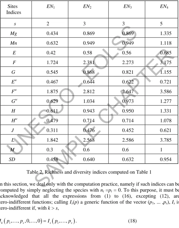
(0.7,0.3,0,0) is sensible only if two species, which could virtually be present in the community, and/or could be found out in a complete census, have not been observed. If this is the case, the vector (0.7,0.3,0,0) is much more informative than the vector (0.7,0.3) for comparison purposes : the first vector displays a community quite concentrated in only two species, while the second shows a community constituted of only two species, at an intermediate level between maximum concentration and evenness.

Sites Indices EN1 EN2 EN3 EN4 s 2 3 3 5 Mg 0.434 0.869 0.869 1.335 Mn 0.632 0.949 0.949 1.118 E 0.42 0.58 0.56 0.685 F 1.724 2.381 2.273 3.175 G 0.545 0.868 0.821 1.155 Ew 0.467 0.644 0.622 0.721 Fw 1.875 2.812 2.647 3.586 Gw 0.629 1.034 0.973 1.277 H 0.611 0.943 0.950 1.331 Hw 0.479 0.714 0.714 1.078 J 0.311 0.476 0.452 0.621 L 1.842 2.568 2.586 3.785 M 0.3 0.6 0.6 1 SD 0.458 0.640 0.632 0.954

Table 2. Richness and diversity indices computed on Table 1

In this section, we deal only with the computation practice, namely if such indices can be computed by simply neglecting the species with ni =pi = 0. To this purpose, it must be acknowledged that all the expressions from (1) to (16), excepting (12), are zero-indifferent functions; calling Is(p) a generic function of the vector (p1, ... ,ps), Is is

zero-indifferent if, with k > s,

(

1, , , 0, , 0

)

(

, ,

k s s 1 s

)

I p … p … =I p … p . (18)

The index M(p), instead, is not zero-indifferent, although being a symmetric function of the pi’s, so also the species with pi = 0 have a direct impact on the index (on the

(9)

UNESCO - EOLSS

SAMPLE CHAPTER

assumption that the four environments hypothesized are “similar”, in the sense that any species could be represented in each of them). The index J(p) is not zero-indifferent in that it is already exactly normalized between 0 and 1, and the normalization procedure takes into account all the species which are necessary to consider for comparative purposes, also the species which - in a particular site - have no representative.

One of the aims in presenting the computations in Table 2 - as well as in the following Tables 3 and 4 - is just to display the remarkable differences between the values assumed by the diversity indices, although very simple and not extreme examples are used. This does not mean that one could choose an index at random - for use in a particular instance; not even, this multiplicity of indices can make us dejected. Just as in the choice of a particular average - e.g. arithmetic, geometric, harmonic, quadratic, median, mode, specific percentiles etc. - the choice of a diversity index should be addressed by the aims of the study, taking into account the formal properties of the indices (at least those properties judged important by the research worker).

According to the coherence properties (4a) and (4b), the sites EN2 and EN3 are not

comparable (a deeper explanation will be provided at Section 2.1), in the sense that neither EN2 is more diverse than EN3, nor EN2 is less diverse than EN3 (given that the two

communities do not coincide); in such a case, two diversity indices are not bound to show the same behavior when passing from one site to the other. Actually, although the values are very near to one another, indices of Gini-Simpson type and indices of Shannon type display an opposite behavior.

This same kind of non-comparability between abundance vectors applies also in a well-known example by Hurlbert (1971, p. 579; Peet, 1974, p. 297): Hurlbert uses a community A with s = 6 and frequencies ni = 18,000 for i = 1,2, ni = 16,000 for i = 3, 4, 5, 6, and a community B with s = 91 and frequencies n1 = 40,000, ni = 667 for i = 2, ... , 91. The calculation of indices F(p) and H(p) gives for community A: F = 5.981 and H = 0.777; for community B Hurlbert erroneously reports F = 5.00 and H = 2.70, showing a quite contrasting behavior, while the exact values are F = 6.101 and H = 1.465.

1.3 Richness

As already stressed, a diversity index combines two aspects of diversity, (1) richness and (2) evenness (or equitability). Both these concepts are not easy to manage; also the simpler concept of richness is not autonomous, as it depends on the number N of individuals (or the total biomass), as well as on the time and effort applied in the specific research. The interpretation of evenness, in its turn, is strictly dependent on the richness s, hence the idea of decomposing a diversity index in two independent contributions is perhaps a delusion. Everybody acknowledges that perfect evenness has a quite different interpretation in the presence of a hundred species, or in the presence of only two or three species, with the unexpected saltus when passing from two species to one species, in which case we speak of perfect homogeneity.

The simpler, most important, although dirty determination of the richness, is the number s

of species actually observed; of course, in comparing s values, care must be taken in considering the total number N of individuals, especially when such values are quite

(10)

UNESCO - EOLSS

SAMPLE CHAPTER

different. When a number k of communities (of the same kind) are analyzed, fixing a common reference value sc for the number of species can be a very useful device in order to ensure a direct comparability of the diversity indices calculated on each experience. Such a common value could be simply sc = max s (among the k communities), as done for the Tables 2 and 3, or it could be derived from some inference about the whole communities (not completely censused), or about the random mechanism contrived for the appearance of new species.

Some problems arise. First, the inferences just mentioned are usually very difficult and very questionable; as Peet (1974, p. 299) observes, knowledge or reliable calculation of the “universe” species number “is close to impossible to determine for most ecological applications”. Besides, the common reference value sc must possess (a) a substantial meaning, and (b) a formal meaning.

About the substantial meaning, it seems obvious that assuming sc = 5 - for instance - when the number of observed species is 3, is sensible only if we are practically certain that two more species are present (although not yet observed), or could easily be present, given the environmental conditions. Lacking this substantial condition, no formal overstress should be admitted. Given a substantial meaning, formal problems could arise all the same. For example, if sc = 15 and N = 10 (for a particular community), the most even abundance vector, consisting of ten one’s and five zero’s, could not reflect all the 15 species, and is consequently bound to formally maintain a certain degree of concentration in some of the species. A stronger limitation of this kind could arise if we are not willing to accept a perfectly even distribution among the set of admissible distributions. A specific proposal to assume as standard the evenness of the so-called “broken stick” distribution has been made by Lloyd and Ghelardi (1964) (cf. Pielou, 1975, p. 17); this and other like proposals, as a preliminary condition, require to be verified for all the communities under study.

1.4 Evenness and Normalization of Diversity Indices

Taking into account the different situations and the different meanings of evenness, two different classes of evenness (concepts and corresponding measures) will be identified: (a) the evenness of first kind, which corresponds to the evenness (without further qualifications) as usually meant in the literature, relates only to the different ways of apportioning the total number of individuals (or the total biomass) among the number of species which are present in each particular community; the indices of this kind need not possess the properties of a diversity index, and actually they are not diversity indices; (b) the evenness of second kind establishes as a common reference the same, real or virtual, number of species sc for all the communities to be compared, thus allowing for a

direct comparison between all the (similar) experiences; the indices of this kind maintain all the properties of a diversity index, though their values are more clearly interpretable as more or less near to the situation of perfect evenness when the maximum number of species is admitted for every community.

Starting from a diversity index, the usual way of deriving an evenness index consists in the process of normalization of the diversity index, using the device

(11)

UNESCO - EOLSS

SAMPLE CHAPTER

( )

min

( )

max min N I p I p I p I p I − = − p (19)

The minimum and maximum of the diversity index I(p) depend on the total number of species which is envisaged; if the number of species is s = number of species present in each site, the normalized index is an evenness index (of the first kind); if such value, instead, is the number sc of the species virtually present in all the sites, we obtain an evenness index of the second kind. In the former case, the values of the indices cannot be compared independently of joint consideration of the richness of each site; in the latter case instead, the indices maintain (with exceptions to be made precise shortly) all the properties of the diversity indices, being simple (linear) increasing functions of the original indices. Actually, such a condition is not exactly satisfied for w-indices, which are functions of the absolute frequencies; the maximizing reference is a vector with five 2’s for the first three sites, and five 4’s for the last one. Considering, for example, the

w-version of the Gini-Simpson index, max Ew is 0.889 for the first three sites and 0.842 for the fourth site, thus a perfect comparability between all sites is impossible if a function of N - beside s - is employed.

The results of the above normalizations, of the first and second kind, are reported in Tables 3 and 4. For completeness, they have been effected also for the three richness indices; however, it must be admitted that such a procedure is rather doubtful (especially for Mg and Mn); a pseudo-normalization has been implemented, consisting only in dividing such indices for the index computed for the maximum s (= 5 in Table 1). As expected, the evenness values in Table 3 - within each row - show a limited spread for many indices, indicating that the evenness of the four communities is more or less of the same degree; quite a different picture comes from Table 4, where the zero frequencies and proportions yield a lowering of the indices, indicating greater homogeneity and less diversity. Sites Indices EN1 EN2 EN3 EN4 Ns1 1 1 1 1 NMg1 1 1 1 1 NMn1 1 1 1 1 NE1 0.84 0.87 0.84 0.856 NF1 0.724 0.690 0.636 0.544 NG1 0.786 0.790 0.747 0.718 NEw1 0.840 0.879 0.849 0.856 NFw1 0.700 0.659 0.599 0.485 NGw1 0.776 0.782 0.736 0.692

(12)

UNESCO - EOLSS

SAMPLE CHAPTER

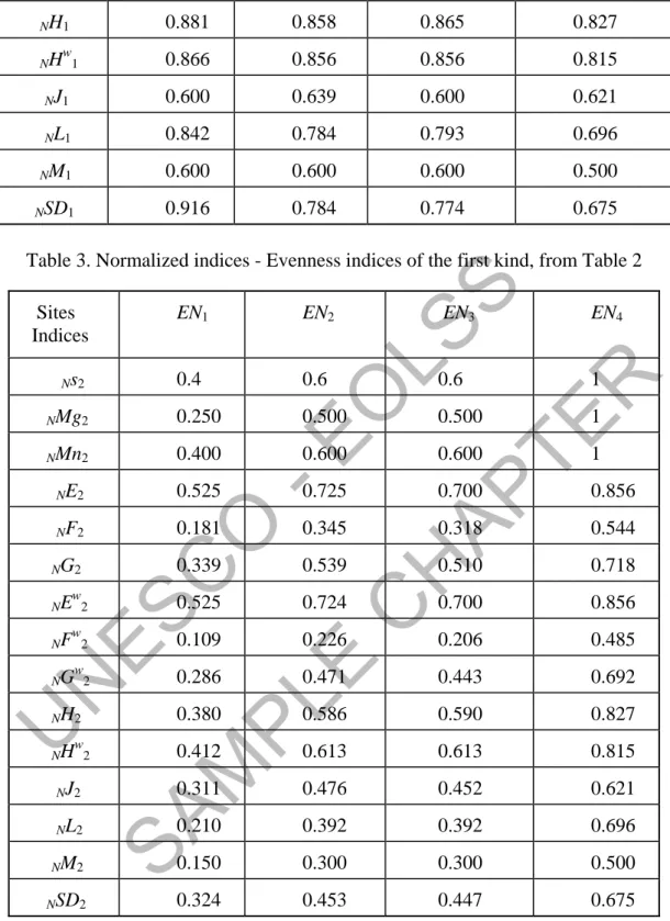
NH1 0.881 0.858 0.865 0.827 NHw1 0.866 0.856 0.856 0.815 NJ1 0.600 0.639 0.600 0.621 NL1 0.842 0.784 0.793 0.696 NM1 0.600 0.600 0.600 0.500 NSD1 0.916 0.784 0.774 0.675

Table 3. Normalized indices - Evenness indices of the first kind, from Table 2 Sites Indices EN1 EN2 EN3 EN4 Ns2 0.4 0.6 0.6 1 NMg2 0.250 0.500 0.500 1 NMn2 0.400 0.600 0.600 1 NE2 0.525 0.725 0.700 0.856 NF2 0.181 0.345 0.318 0.544 NG2 0.339 0.539 0.510 0.718 NEw2 0.525 0.724 0.700 0.856 NFw2 0.109 0.226 0.206 0.485 NGw2 0.286 0.471 0.443 0.692 NH2 0.380 0.586 0.590 0.827 NHw2 0.412 0.613 0.613 0.815 NJ2 0.311 0.476 0.452 0.621 NL2 0.210 0.392 0.392 0.696 NM2 0.150 0.300 0.300 0.500 NSD2 0.324 0.453 0.447 0.675

Table 4. Normalized indices - Evenness indices of the second kind, from Table 2

2. General Properties of Diversity Indices 2.1. Statistical Proposals of General Properties

Around the seventies of the twentieth century, several studies appeared concerning the

(13)

UNESCO - EOLSS

SAMPLE CHAPTER

general properties of some classes of descriptive statistical indices; only for averages (or mean values), and inequality (or concentration) measures, similar proposals had been made by some statisticians and economists much earlier. However, as concerns diversity indices, it was easily recognized that their structure was the same already established for inequality measures. In the Italian statistical literature, this was a natural continuation of the proposal, made by Gini (1918) and Leti (1965), of the Gini’s concentration ratio as a measure of the heterogeneity of a categorical or qualitative variable.

In two connected papers, Herzel (1967, 1968) deals with the general properties of the measures of dispersion, concentration and heterogeneity. By a thorough examination of some indices of common use, he establishes the following conditions for any diversity index g: (1) as a function of the relative frequencies, or the probabilities, pi of the s classes,

g must be $ 0, and equal to zero only when pi = 1 for one class (the others being zero); g

must be symmetric with respect to the independent variables; (3) max g corresponds to the case when pi =1/s for i = 1, ... , s; in the case of perfect heterogeneity, g must be an increasing function of s. In the second paper, Herzel (1968) points out that “the principal indices of heterogeneity are symmetric concave functions”; hence, he also includes concavity among the typical properties of these indices. Moreover, he dwells upon the apparent duality existing between homogeneity indices and measures of concentration or inequality, already noticed by Gini and Leti.

In 1975, while a related paper on general descriptive statistics is being published by Bickel & Lehmann, Peccati & Riva suggest the following coherence property for diversity indices:

given distributions p = (p1, ... ,ps), p’ = (p1’, ... ,ps’), and A = (1/s, ... ,1/s), such that

1 1 1,

i i ,

p′ − s ≤ p − s i = … s (20)

a diversity index I(p) must be order preserving, i.e. I(p) # I(p’); in other words: the nearer the distribution p to the equalizing point A, the higher (or at least not lower) the diversity of p.

In the following year, Frosini (1976a,b) proposes a stronger coherence property for diversity indices; two equivalent expositions are as follows:

Tendency to a more even distribution: given p = (p1, ... ,ps), with pr < ps, another distribution p’ is obtained such that pi’ = pi for i … r,s, pr’ = pr + d, ps’ = ps - d being d > 0 and pr’ # ps’; a diversity index I(p) must satisfy I(p) # I(p’).

Tendency to a more concentrated distribution: given p’ = (p1’, ... ,ps’), with 0 < pr’ # ps’,

another distribution p is obtained such that pi = pi’ for i … r,s, pr = pr’ - d, ps = ps’+ d (d > 0); a diversity index must satisfy I(p) # I(p’).

This criterion determines a partial ordering of distributions comparable to a given one. Perhaps this is more appealing by working with absolute frequencies; for example, if we compare the distributions (7,3,0) and (5,4,1) (same total 10), it is evident how the second distribution can be obtained from the first one by means of two successive transfers, lowering the first frequency and raising the other two, thus attaining a greater heterogeneity (or diversity). Instead, the distributions (6,2,2) and (5.4.1) do not belong to

(14)

UNESCO - EOLSS

SAMPLE CHAPTER

the same partial ordering: in fact, the second is obtained, starting with the first one, by applying both a lowering and a raising of frequencies. Thus, (7,3,0) belongs to the partial ordering generated by (5,4,1), but (6,2,2) does not.

As a general definition, two distributions p and p’ are comparable if and only if we can pass from one to the other by means of a finite number of transfers of the same kind (all tending to equalize the frequencies, or all tending to the opposite purpose). As an implication, we can recognize the two extremal distributions of every partial ordering of relative frequencies or proportions; the distribution A = (1/s, ... ,1/s) of maximum heterogeneity (or minimum homogeneity), and the distribution (1,0,...,0) - or one of its permutations - of minimum heterogeneity (or maximum homogeneity).

The above property can be re-expressed for the complementary concept (and measures) of homogeneity: an index of homogeneity C(p) must increase (or at least not decrease) if we pass to more homogeneous distributions, by raising larger pi’s at the expense of lower

pi’s.

With such definitions, it is easy to control, if I is a diversity index, that the same holds for

f(I), being f a monotonically increasing function (defined on the domain of the values taken by I, and having as co-domain a subset of the non-negative reals). An analogous statement holds true if we refer to a homogeneity index C: f(C) is a homogeneity index all the same. It is easy to control that a decreasing function of a diversity index produces a homogeneity index, and vice versa.

The above partial ordering is able to deal also with the comparability of vectors, when some frequencies or proportions are zero, for example the vectors (7,3,0) and (5,4,1); as the zeros can only be increased by some transfer of frequencies or proportions, the vector with a smaller number of zeros has to display greater heterogeneity in order that the vectors belong to the same partial ordering (“either the community with the larger number of species is more diverse or the communities are not comparable”, Solomon, 1979). An implication is that, considering two perfectly even distributions, one with s

non-zero proportions and the other with k > s non-zero proportions, the latter displays a greater heterogeneity, as is obtained from the former by a series of “egalitarian” transfers, directed to lower s proportions from 1/s to 1/k, and to raise (k-s) proportions from zero to 1/k. Hence, a diversity index should increase when passing from the former vector to the latter.

2.2. Diversity and Inequality

The above definition of homogeneity indices formally coincides with the definition of quite another kind of statistical summary measures, that is, inequality - or concentration - indices (whose basic defining property was established by Dalton in 1920); such indices are usually applied to income or wealth distributions. Absolute income distributions for N

individuals are indicated by x = (x1, ... ,xN), with xi $ 0, 3 xi = T (total income), while

relative income distributions are indicated by q = (q1, ... ,qN), qi = xi / T, 3 qi = 1, where xi

is the income of the i-th individual and qi is the share of the total income pertaining to him. It is customary to arrange the incomes - and corresponding shares - in ascending order of

(15)

UNESCO - EOLSS

SAMPLE CHAPTER

magnitude, that is, qi # qi+1.

A partial ordering of (comparable) income distributions is obtained from a given distribution q by successively performing egalitarian transfers (from a richer individual in favor of a poorer one), or non-egalitarian transfers (the opposite redistribution). A concentration or inequality measure must preserve this ordering, thus it must increase (or at least not decrease) by successively passing towards more concentrated - or unequal - distributions. It is then evident that order preserving functions for the concentration of income distributions are the same order preserving functions for the homogeneity of a categorical distribution. As an immediate consequence, all the measures devised to summarize the inequality of income distributions can be utilized as diversity indices, at least in the sense of evenness indices; some main examples will be examined in the sequel.

The reservation made in the last sentence needs some explanation. In introducing the concept of diversity in Section 1.1, it was esteemed essential, for a diversity measure, to be sensitive to the number of species (or classes) observed in a community; this is obviously taken for granted for the simple index coinciding with s, but in no way is it obvious for other indices. On the contrary, it is generally shared among the economists (cf. Sen, 1973), that income inequality measures be independent from the number N of individuals; beside theoretical considerations, this is certainly affected by the large dimensions of the samples or populations usually analyzed. More precisely, if we put together - i.e. make a mixture - of h populations which are replicas of one and the same population, the judgment about the concentration of incomes must be unchanged with respect to each of the component populations. For some inequality measures, we can be content with an approximate equality, which is practically satisfying - in any case - when the number of individuals exceed a thousand. Inequality indices not depending on N can be translated in homogeneity (hence diversity) indices not depending on s, thus producing a class of indices not suitable for summarizing species diversity, but only suitable for summarizing evenness.

However, among statistical concentration studies there is a field - that of industrial concentration - asking for indices highly dependent on the number of firms in a market (Theil, 1967); these are precisely the indices which parallel the indices of homogeneity, and - by means of simple transformations - the diversity indices. Perhaps the most important index in this group is an application of formula (4); in this kind of applications it is usually called Herfindhal index:

( )

2

i

D q =

∑

q (21)

Let us see what happens if, from a population PN with N individuals, we derive another population PhN, composed of hN individuals, derived from PN by equally sharing each qi among h individuals; the index D can be written

( )

2 2

(

1 1 1 1 1 h N _s N hN s N q D P q D P h h h ⎛ ⎞ = _⎜ _⎟ = = ⎝ ⎠

∑ ∑

∑

)

(22)

(16)

UNESCO - EOLSS

SAMPLE CHAPTER

For example, this result means that the mixture of two populations identically distributed halves the concentration measured by D on each of the two component populations. Translated for homogeneity indices, this means that

( )

1

( )

hs s

D P D P h

= (23)

i.e. the distribution

(

p h1 ,…,p h p h1 , 2 ,…,p h p h2 , s ,…,p hs

)

brings out a homogeneity index D which equals D(p1, ... ,ps) divided by h. Turning to the

diversity index E = 1 - D, it is obtained

( )

1

( )

1 1 hs hs s s E P D P D P E h = − = − > P (24)

namely, the mixture is more diverse than the original distribution.

It is important to correctly interpret the above result. Let us think of two populations, each with three species and the same relative abundance vector p = (0.5,0.3,0.2), with respective absolute abundance vectors a1 = (50,30,20) and a2 = (10,6,4); the mixture of

the two populations, under the hypothesis that such populations do not have any species in common, gives rise to the following absolute abundance vector: a1+2 =

(50,30,20,10,6,4), with corresponding relative abundance vector (0.417,0.25,0.167,0.083,0.05,0.033); the value of D computed on the vector p is 0.38, while D computed on the mixture is 0.274. It should be clear that, when we speak of a mixture of identically distributed vectors in the above context, we mean to refer to

absolute abundance vectors. Following the example, if both populations possess the absolute distribution a2, the mixture has absolute distribution (10,10,6,6,4,4), with

relative distribution (0.25,0.25,0.15,0.15,0.10,0.10) and D = 0.19 = 0.38/2.

Concerning the above mixture, the Shannon index (14) displays the following behavior:

( )

1 1

1

log

log log log

h s _i _i hs s i i s p p H P h h s p p h H P h H ⎛ ⎞ = − _⎜ _⎟ ⎝ ⎠ = − + = + >

∑ ∑

∑

P (25)

with a result analogous to (24): the diversity computed on the mixture is greater than the one computed on the original distribution.

2.3 Majorization and Lorenz Curve

In section 2.1, by quoting Herzel (1968), it was recognized that a property of the most usual diversity indices - such as Gini-Simpson E and Shannon H - is their concavity

(17)

UNESCO - EOLSS

SAMPLE CHAPTER

(while corresponding homogeneity and concentration indices are convex functions). In a subsequent paper, Herzel (1977) relaxes such conditions to quasi-concavity and quasi-convexity, as it can be shown that - as far as we are concerned with comparable vectors - only quasi-concavity (or quasi-convexity) appears of interest (Frosini, 1987,, pp. 86-87). Anyway, the very meaning of the coherence property introduced in Sections 1.1 and 2.1, and the relative easiness to check it in particular instances, have maintained the general reference in the statistical literature to functions which are order preserving with respect to comparable distributions: such functions are called Schur-concave functions, or simply S-concave functions (cf. Marshall & Olkin, 1979). On the other hand, any concave (convex) function is quasi-concave (convex); symmetric quasi concave (convex) functions are S-concave (convex), thus the set of S-concave (convex) functions is the most inclusive and less demanding; actually, the set of S-concave functions includes functions which are - loosely speaking - “quasi convex” (Frosini, 1976b, 1987; Forcina & Giovagnoli, 1982).

The formal characterization of S-concave functions is usually made through majorization. Given two vectors p and q:

(

1, , s

)

, 1 s 0, i 1;

(

1, , s

)

, 1 s 0,

p= p … p p ≥…≥ p ≥

∑

p = q= q … q q ≥…≥q ≥

∑

q_i =1 we say that p majorizes q, and write p š q (or q ˜ p) if the following (s - 1) inequalities are satisfied: 1 1 1, , 1 j j i i p ≥ q j = s

∑

… − (26) or equivalently if 2, , s s i i jp ≤ jq j= s

∑

… (27)

The same majorization criterion is also directly applicable to absolute abundance vectors, provided the totals of individuals coincide. For example, if p = (11,5,3,1) and q = (16,2,1,1) (obtained from p by means of two non-egalitarian transfers), the partial sums of type (26) compare as follows:

p 11 16 19 20

q 16 18 19 20

and the partial sums of type (27) compare as follows:

p 1 4 9 20

q 1 2 4 20

It is easily checked that a succession of non-egalitarian transfers, tending to produce a more concentrated distribution, is equivalent to pass from p to new vectors p’, p”, ... , majorizing it: p ˜ p’ ˜ p” ˜ ... (the opposite happens when egalitarian transfers are applied). Given two generic vectors p and q as above, a function f such that

(18)

UNESCO - EOLSS

SAMPLE CHAPTER

( )

implies

p q f p ≥ f q (28)

is S-convex; and a function f such that

( )

implies

p q f p ≤ f q (29)

is S-concave. Therefore, as far as comparable vectors are concerned, an S-concave function is an order preserving function of the inverse majorization ordering (which is completely equivalent with the coherence property of Section 2.1). As it is a very natural requirement, it is no surprise that practically all diversity indices - intentionally or not - proposed in the literature (and the most important indeed) are S-concave functions (cf. Solomon, 1979).

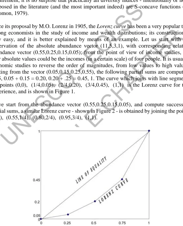
Since its proposal by M.O. Lorenz in 1905, the Lorenz curve has been a very popular tool among economists in the study of income and wealth distributions; its construction is very easy, and it is better explained by means of an example. Let us start with the observation of the absolute abundance vector (11,5,3,1), with corresponding relative abundance vector (0.55,0.25,0.15,0.05); from the point of view of income studies, the four absolute values could be the incomes (in a certain scale) of four people. It is usual in economic studies to reverse the order of magnitudes, from low values to high values; starting from the vector (0.05,0.15,0.25,0.55), the following partial sums are computed: 0.05, 0.05 + 0.15 = 0.20, 0.20 + .25 = 0.45, 1. The curve which joins with line segments the points (0,0), (1/4,0.05), (2/4,0.20), (3/4,0.45), (1,1) is the Lorenz curve for this experience, and is shown in Figure 1.

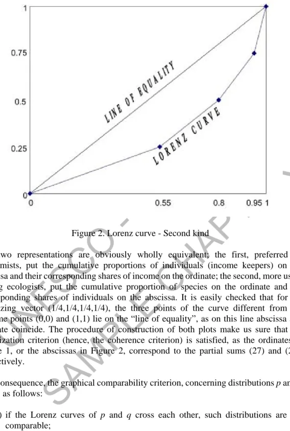
If we start from the abundance vector (0.55,0.25,0.15,0.05), and compute successive partial sums, a similar Lorenz curve - shown in Figure 2 - is obtained by joining the points (0,0), (0.55,1/4), (0.80,2/4), (0.95,3/4), (1,1).

Figure 1. Lorenz curve - First kind

(19)

UNESCO - EOLSS

SAMPLE CHAPTER

Figure 2. Lorenz curve - Second kind

The two representations are obviously wholly equivalent; the first, preferred by economists, put the cumulative proportions of individuals (income keepers) on the abscissa and their corresponding shares of income on the ordinate; the second, more usual among ecologists, put the cumulative proportion of species on the ordinate and the corresponding shares of individuals on the abscissa. It is easily checked that for the equalizing vector (1/4,1/4,1/4,1/4), the three points of the curve different from the extreme points (0,0) and (1,1) lie on the “line of equality”, as on this line abscissa and ordinate coincide. The procedure of construction of both plots make us sure that the majorization criterion (hence, the coherence criterion) is satisfied, as the ordinates in Figure 1, or the abscissas in Figure 2, correspond to the partial sums (27) and (26), respectively.

As a consequence, the graphical comparability criterion, concerning distributions p and q, works as follows:

(a) if the Lorenz curves of p and q cross each other, such distributions are not comparable;

(b) if the Lorenz curve of p lies below (at least in some range of the curve) the Lorenz curve of q, then we can say that p is more concentrated, or equivalently that q is more evenly distributed.

It is easy to check that the distribution q used above, with absolute abundance vector (16,2,1,1), and relative vector (0.80,0.10,0.05,0.05), lies below the curve of the distribution p, and in fact can be obtained from p through two non-egalitarian transfers.

(20)

UNESCO - EOLSS

SAMPLE CHAPTER

On the other hand, if we use anew an example already exploited in Section 2.1, it is easily checked that the absolute distributions p = (6,2,2) and q = (5,4,1) are not comparable; in fact, their partial sums of type (26) are 6, 8, 10 for p, and 5, 9, 10 for q, hence their Lorenz curves cross each other.

It is quite evident that any comparison between two or more distributions is mostly significative if totals of individuals and numbers of species are constant over all the communities under study. Relative figures, such as proportions or percentages, are useful and practically indispensable, but it is only too obvious that the absolute distributions (11,5,3,1) and (110,50,30,10) have a quite different meaning. As the Lorenz plot uses proportions in both coordinates, we begin with the observation that - in the comparison of Lorenz curves - one should not lose sight of the absolute values of the individuals for each species.

However, the most disturbing fact is that the Lorenz curve is wholly independent (except for the number of points inserted on the curve) of the number of species. To this end, it is useful to recall, from Section 2.2, what happens when the proportions of each species are equally divided into h sub-species; it is easy to see that the original Lorenz curve remains unchanged after the subdivision, only (h - 1) new points appear on each of the original line segments. As observed by Taillie (1979, p. 55), referring to the case h = 2, “it seems plausible that combining these communities should give a community with the same evenness but twice the richness as either of the original communities”. Thus, one must be careful to extract from a Lorenz plot only a sight of the evenness of a distribution. In view of not losing important pieces of information, absolute values for one or both the coordinate axes could be used.

3. Special Indices and Families of Indices 3.1. Gini-Simpson Indices and Generalizations 3.1.1. Derivation of the Gini-Simpson Index

In an article of 1912, Gini works out several formulae aiming at establishing suitable indices of variability for qualitative phenomena (or categorical variables), quite analogous - as far as possible - to the ones well-known for quantitative variables, which are measured at least on an interval scale. One such index is directly derived from the variability measure most investigated and applied by Gini, namely the (Gini’s) mean difference (of order one). With respect to observations x1, ... , xN of a quantitative variable

X, organized in a frequency distribution with distinct values x1’, ... , xs’, respective

absolute frequencies n1, ... , ns, and relative frequencies p1, ... , ps (pi = ni/N), the mean

∑ ∑

− =

∑ ∑

− p p

If we put | xi’ - xj’ | = di j, and interpret di j, for the case of qualitative variables, as the

(21)

UNESCO - EOLSS

SAMPLE CHAPTER

distance between the categories xi’ and xj’, MD assumes the following form: ij i j

MD=

∑∑

d p p

)

(30) At this point Gini assumes the uniform distance 1 between any two different categories,

being obviously di i = 0 for i = 1, ... , s; formula (30) is then simplified as

(

)

2

(

1 1 1 1 s s i j i i i i j MD p p p p p E ≠ =

∑

=

∑

− = −

∑

= p

)

(31)

giving rise to the index now known as Gini-Simpson index. Leti (1965) suggests that the value (1 - pi) may be considered as a measure, relative to one unit of the population, of the heterogeneity of the i-th category; therefore we are allowed to take their mean as a measure of the heterogeneity of the whole population.

Another natural way of looking at the index E (formula (5)) is the one proposed by Simpson (1949); actually, D(p) = 3 pi2 is the probability that two successive independent drawings (of individuals) from the population characterized by the abundance vector p = (p1, ... ,ps) yield units belonging to the same species; Simpson correctly describes D(p) as

a measure of concentration (of the classification). In a complementary way, E(p) = 1 - 3 pi2 is the probability that two independent drawings yield units belonging to different species, so E(p) is a measure of diversity of the classification. I.J. Good (1982) quotes from A.M. Turing the natural name of repeat rate for the concentration index D(p). If the procedure of successively drawing units from the population is accomplished

without replacement (i.e. the more informative way of sampling, compared to sampling

with replacement), the above expression for the repeat rate changes accordingly, and the Gini-Simpson index becomes

( )

(

)

1 1 1 1 1 s i i w w i n n E p D p N N = − = − = − −

∑

(32)

In many applications Ew •E; this is perhaps clearer with the equivalent expression

( )

2 1 1 1 1 1 s w i i N E p p N = N = − + −

∑

− (33)

The equation of a sphere with radius c, in a euclidean space of s dimensions, centered at the point A = (1/s, ... ,1/s) is:

2 2 2 1 1 1 1 s s i i i i p p s s = = ⎛ ₋ ⎞ ₌ _{− =} ⎜ ⎟ ⎝ ⎠

∑

c

Therefore, within the domain characterized by the inequalities pi $ 0, i = 1, ... , s, and 3 pi = 1, such spheres - or portions of such spheres - are level surfaces of D(p) and E(p).

(22)

UNESCO - EOLSS

SAMPLE CHAPTER

3.1.2. A family of IndicesDepending on the Euclidean Distance

Several diversity indices have been proposed, which are increasing functions of E or Ew, or decreasing functions of D or Dw; some of them are reported in Section 1.2. On the other side, these indices can be recognized as special instances within families of indices. One such family was proposed by Frosini (1976b, p. 523), generalizing the fair, or neutral index J; the general index in this family is simply derived from (12) by raising to the exponent α the normalized euclidean distance d(p,A):

( )

1 M d J p d α α α ⎛ ⎞ = −_⎜ _⎟ > ⎝ ⎠ 0 Δ (34)

as 0 # d/dM # 1, α = 1 determines the fair index J1 = J, while 0 < α < 1 and α > 1 yield a

finer discrimination between distributions p, respectively, in a neighbourhood of A = (1/s, ... ,1/s), or in proximity of the extremal distributions of type (1,0, ... ,0). Other similar families can be easily constructed by starting with other kinds of distances (see Section 3.2).

3.1.3. Rao’s Family based on Dissimilarity Coefficients

Formula (30) is immediately recognized as a quadratic form, with matrix Δ = [dij]; the generalization is obviously of the type

( )

ij i j

H_Δ p =

∑∑

d p p = p p′ (35) with p a column vector, and dij being the distance, or dissimilarity between two generic

categories or species (Rao, 1982a,b; 1986). In order to exploit such diversity measure not only with respect to one population or community, but also with respect to mixtures of populations, Rao proposes for HΔ(p) the strong condition that it be a concave function

over the domain {p : pi$ 0, 3 pi = 1}, “so that the diversity in a mixture of distributions is not smaller than the average diversity of the individual distributions constituting the mixture” (Rao, 1982a, p. 6).; moreover, the diversity measure should attain its minimum zero in case of perfect homogeneity. The ensuing restrictions on the elements dij are as follows:

(a) d11 = ... = dss

(b) the (s - 1)x(s - 1) matrix with elements (dik + djk - dij - dkk), i,j = 1, ... , k - 1, is non-negative definite.

Although demanding a large supplementary effort to the research worker, who is asked to establish dissimilarities (hopefully objectively based) between species, this approach is potentially suitable to take into account the graduation in likeness between different species.

(23)

UNESCO - EOLSS

SAMPLE CHAPTER

3.2. Diversity Indices based on Distances between Distributions

Although most diversity indices, loosely speaking, can be viewed as functions of the

distance, somewhat defined, between a distribution p = (p1, ... ,ps) and the uniform distribution A = (1/s, ... ,1/s), only some special indices are defined according to the properties usually attached to a geometrical or topological distance. As seen at Section 3.1.2, one index of this kind is J, and its generalization Jα, based on the euclidean

distance; the level surfaces of Jα (p), defined as the sets of points in the s-dimensional

space Rs which determine the same value of the index, are in this case the surfaces of spheres (for s $ 4), which reduce to circles for s = 3 (N.B. only points of the hyperplane 3 pi = 1 must be considered).

This geometrical approach has the advantage of leading to a distinct consideration of: • the level surfaces, or equivalent classes, defined by the sets S(c) = {p : pi $ 0, 3 pi

= 1, I(p) = c}; if two distributions belong to the same equivalent class, it means that they are declared equivalent from the diversity viewpoint;

• the value I(p) attached to the continuum of the equivalent classes.

Thus, if we look at the indices E, F, G and the family Jα , we recognize that all the indices

are constant over spheres, i.e., they assume the same value for two distinct distributions when they have the same euclidean distance from A. If such is the case, we can pass from one index to another by means of increasing functions.

Another general kind of distance, which could be examined, is the Minkowski distance

(

)

1 , 1 r r r i d p A =⎡_⎣

∑

p − s ⎤_⎦ (36)

The two kinds of distances most used, beside the euclidean distance, are the city-block distance

(

)

1 , i

d p A =

∑

p −1 s (37)

and the ultrametric distance

(

,

)

max1 1

u i s

d p A = _{≤ ≤} p_i − s ; (38)

they are homogeneity indices, which take values - respectively - between 0 and 2(s - 1)/s, 0 and (s - 1)/s (Frosini, 1981). Diversity normalized indices are therefore:

( )

(

)

1 1 2 1 i s B p p s s = − − −

∑

(39)

( )

1 1 max 1 i s U p p s s = − − − (40)

(24)

UNESCO - EOLSS

SAMPLE CHAPTER

For s = 3 the level curves for both indices are hexagons centered in A.

The same kinds of distances could be applied by comparing a given distribution with its

opposite (Frosini, 1981). For example, if p = (0.6,0.3,0.1), its opposite is q = (0.1,0.3,0.6). Letting the values pi ordered from largest to smallest, as usual in ecological studies, the values qi are ordered from smallest to largest; the square of the euclidean distance between p = (p1, ... ,ps) and its opposite q = (ps, ... ,p1), is

(

)

(

)

2 2 1 1 , s i s i i d p q p p_{− +} = =

∑

− (41)

while the city-block distance is

(

)

1 1 , s i s i i d p q p p _{− +} = =

∑

− 1 ; (42)

both distances share the properties of a homogeneity index and take values between 0 and 2; the construction of normalized indices is therefore immediate.

3.3 Shannon and Entropy Measures

One of the best known diversity indices, the entropy or Shannon index (formula (14)), shares all the properties required to such indices, but it derives from a mathematical characterization and application problems very far from the characterization of the variability of a categorical variable and the ecological diversity; such a measure was introduced by Shannon (1949), using logarithms with base 2, within the theory of information, or communication. Actually, the methodological contents of this measure are easily seen to have a larger scope; the entropy (14) is aimed at measuring “the amount of uncertainty of the distribution V, that is, the amount of uncertainty concerning the outcome of an experiment, the possible results of which have the probabilities p1, p2, ... ,

pn” (Rényi, 1961, p. 547). This wide characterization is, in effect, the characterization of a heterogeneity or diversity index, while some mathematical conditions imposed on the entropy function are strictly related to its use in the information context. Something like happens with the Brillouin index (16), which is the “finite population” version of the Shannon index (Pielou, 1975, p. 10).

A well-known generalization of the Shannon index is the “entropy of order α” of the distribution p:

( )

1 log 0, 1 1 i H_α p pα α α α = −

∑

> ≠ (43)

usually ascribed to Rényi (1961) (but also ascribable to I.J. Good - see Patil & Taillie, 1982, p. 550). The limit of Hα when α 6 1 turns out the entropy H, which can therefore be

called H1 within this family of entropies.

(25)

UNESCO - EOLSS

SAMPLE CHAPTER

Another generalization, called hypoentropy, was introduced by Ferreri (1980); its expression, depending on a parameter λ, is as follows:

( )

1

(

)

1

(

) (

)

1 log 1 1 log 1 0 i i p p λ _λ λ _λ λ λ ⎛ ⎞ Φ =_⎜ + _⎟ + − + + ⎝ ⎠ >

∑

λp (44)

being H the limit of Φλ as λ 64. Several other entropy expressions exist in the

mathematical and information literature (see e.g. Nayak, 1985; Baczkowski, Joanes & Shamia, 1998).

Another approach was followed by De Simoni (1979), who stressed the interesting properties of the “entropy of degree α ” proposed by Daroczy (1970), observing that some of them (in particular sub-additivity - when α >1 - and the fulfilment of the branching principle) deserve greater attention in the construction and application of diversity measures.

3.4. Diversity Indices Derived from Averages

Most of the diversity or homogeneity indices seen above can be recognized as averages of

rarity measures or abundance measures for each species. For example, as observed by Leti (1965, already quoted in Section 3.1), (1 - pi) may be considered as a measure of the heterogeneity of the i-th species; the arithmetic mean of the quantities (1 - pi) , weighted by pi, gives rise to the Gini-Simpson diversity index E. On the other hand, pi is the natural

measure of the relative abundance of the i-th species: the weighted arithmetic mean of these quantities results in the Gini-Simpson homogeneity index D. The same author, in deriving the index L, observes that, taking the reciprocal 1/pi as a measure of rarity for each category, the weighted geometric mean (with weights pi as above) of these quantities results in the index L.

Following the same approach, Burgio (1969) averages the pi’s by a weighted power mean of order r, thus obtaining the homogeneity index Ar(p) = (3 pir+1)1/r, which takes values between 1/s and 1, just as D(p) = A1(p); putting α = r + 1, a diversity measure is simply

obtained by taking the complement with respect to one: