DATA AND IMPLICATION BASED COMPARISON OF TWO CHRONIC MYELOID LEUKEMIA MODELS

AND ENGINEERING

Volume10, Number5&6, October & December2013 pp.1501–1518

DATA AND IMPLICATION BASED COMPARISON OF TWO CHRONIC MYELOID LEUKEMIA MODELS

R. A. Everett1, Y. Zhao1, K. B. Flores2 and Y. Kuang1

1 _{School of Mathematical and Statistical Sciences} Arizona State University, Tempe, AZ 85287, USA 2 _{Department of Mathematics, North Carolina State University}

Raleigh, NC 27695, USA

Abstract. Chronic myeloid leukemia, a disorder of hematopoietic stem cells,

is currently treated using targeted molecular therapy with imatinib. We com-pare two models that describe the treatment of CML, a multi-scale model (Model 1) and a simple cell competition model (Model 2). Both models de-scribe the competition of leukemic and normal cells, however Model 1 also describes the dynamics of BCR-ABL, the oncogene targeted by imatinib, at the sub-cellular level. Using clinical data, we analyze the differences in es-timated parameters between the models and the capacity for each model to predict drug resistance. We found that while both models fit the data well, Model 1 is more biologically relevant. The estimated parameter ranges for Model 2 are unrealistic, whereas the parameter ranges for Model 1 are close to values found in literature. We also found that Model 1 predicts long-term drug resistance from patient data, which is exhibited by both an increase in the proportion of leukemic cells as well as an increase in BCR-ABL/ABL%. Model 2, however, is not able to predict resistance and accurately model the clinical data. These results suggest that including sub-cellular mechanisms in a math-ematical model of CML can increase the accuracy of parameter estimation and may help to predict long-term drug resistance.

1. Introduction. Chronic myeloid leukemia (CML) is a cancer of the white blood cells. It is a disorder of hematopoietic stem cells characterized by the increased growth of myeloid cells in the bone marrow and the excessive presence of these cells in the blood. CML can be molecularly diagnosed by detecting the presence of the Philadelphia (Ph) chromosome and the fusion oncogene BCR-ABL. This oncogene is the result of translocation of the BCR, or breakpoint cluster, gene located on chromosome 22 and the ABL, or Ableson leukemia virus, gene located on chromosome 9 [3] . The progression of CML consists of three phases. The first phase, called the benign chronic phase, is typically asymptomatic and can last for several years untreated. The accelerated phase then follows and leads to the last phase, called blast crisis, which is characterized by an abnormally high number of stem cells and precursor cells in the blood or bone marrow [1]. CML can advance from the chronic phase to the fatal blast crisis phase in a timespan of 3 to 5 years [3].

2010Mathematics Subject Classification. Primary: 34K20, 92C50; Secondary: 92D25. Key words and phrases. Chronic myeloid leukemia, clinical data, drug resistance, cancer modeling.

This work is supported in part by NSF DMS-0920744.

For CML patients in which the BCR-ABL oncogene is detected, targeted molec-ular therapy can be used to inhibit the growth of stem cells. Imatinib, also known as STI-571 and Gleevec [12], is a tyrosine kinase that binds to the ATP binding site of BCR-ABL kinase, stopping cell-growth signals and decreasing cell proliferation [5]. Previously, treatment options included other drugs, such as hydroxyurea or in-terferon alpha, and allogeneic bone marrow transplants. Imatinib, which is effective in all phases of CML progression, is now a widely used primary treatment option for BCR-ABL positive CML patients [1].

BCR-ABL transcript levels are obtained using quantitative reverse transcription polymerase chain reaction for diagnosis and to determine the effect of treatment [17]. The amount of BCR-ABL transcript is then normalized using some control gene, usually BCR or ABL. Thus the data is presented as BCR-ABL/control gene percentages (BCR-ABL/ABL%) [17,14].

Most CML patients with imatinib treatment exhibit a biphasic profile, which means that the patients exhibit an initial rapid decline followed by a gradual de-cline in BCR-ABL/ABL%. However, some patients exhibit a monophasic or tripha-sic profile. The BCR-ABL/ABL% for a monophatripha-sic profile gradually decline over time. Patients with a triphasic profile can exhibit a rapid BCR-ABL/ABL% decline followed by a relatively gradual ABL/ABL% decline, followed by a rapid BCR-ABL/ABL% increase [18]. The increase in the triphasic profile is most likely caused by mutations in the BCR-ABL gene that encode resistance to Imatinib [18,5,6,7], although gene amplification is also a possible cause for resistance [6]. When treat-ment is stopped, the BCR-ABL/ABL% of some patients rapidly increases to levels at or beyond pre-treatment baseline [13]. There are different hypotheses as to the cause of this increase and mathematical modeling techniques have the potential to be helpful in elucidating the underlying mechanisms of therapy resistance.

Several groups have utilized mathematical modeling to study the effect of tar-geted treatment and imatinib on CML, including Roeder et al. and Michor et al. [17, 13, 11]. Roeder et al. describe a computational model in which cells tran-sition between two environments. In this scenario, stem cells can proliferate and differentiate in one of the environments and are quiescent in the other environment. Roeder et al. demonstrated both a biphasic decline as well as the rapid increase in BCR-ABL/ABL% when treatment is stopped. Roeder et al. hypothesized a degradation of proliferating stem cells during treatment and concluded that ima-tinib treatment can eradicate the disease, assuming no mutations. When treatment is stopped, the relapse can be attributed to the proliferation of dormant stem cells that were not affected by the proliferation-specific degradation effect. Michor et al. proposed a different mathematical model that describes four cellular subpopula-tions in a CML patient: stem cells, progenitors, differentiated cells, and terminally differentiated cells. Michor et al. also demonstrated a biphasic decline as well as the rapid increase when treatment is stopped. Their model incorporated the ex-pansion of imatinib resistant stem cells during imatinib treatment and concluded that leukemic stem cells are not depleted during imatinib therapy and thus imatinib therapy cannot eradicate the disease.

Stein et al. [18] compared different hypotheses of the models described above. Assuming a biphasic decline in BCR-ABL/ABL%, which was demonstrated by both models, there are two slopes: α, which corresponds to the initial rapid decrease and

β, which corresponds to the long-term response. One hypothesis, supported by Roeder et al., was the proliferating-quiescent hypothesis, where α is due to the

proliferating stem cells and β is due to the quiescent stem cells. Another was the late-early progenitors hypothesis, supported by Michor et al., whereαis due to the late progenitor cells and β is due to the early progenitor cells. Stein et al. also considered a third hypothesis, the early stem cell hypothesis, which states thatαis due to a decline of early progenitor cells andβ is due to a decline of late progenitor cells. Stein et al. rejected the late-early progenitors hypothesis and concluded that

β is due to late progenitor depletion. However, the factors contributing to the parameterαare still unknown.

These previous CML models described different cell environments and different cell populations, but not sub-cellular dynamics, which may provide insights into the sub-cellular origins of proliferation and resistance. Recently, Portz et al. [16] de-scribed a cell quota model that describes a treatment for patients with prostate can-cer called intermittent androgen suppression, a hormone therapy. Normal prostate cells as well as most prostate cancer cells depend on androgen signaling for sur-vival and proliferation. Androgen suppression treatment lowers the androgen levels, which prevents the growth of cancer cells. The treatment can be initially success-ful, however most patients experience a relapse. Portz et al. suggest that during the relapse, androgen-independent cells (AI), which can grow in low-androgen lev-els, replace androgen-dependent cells (AD). In their final model, the growth rate of both the AD and AI populations are described by Droops cell quota models, which introduce two new variables to represent the cell quotas for androgen. The switching rates between the two populations are modeled using the hill equations. The marker for prostate cancer, prostate-specific antigen (PSA), is assumed to be dependent on androgen levels in the model. This assumption was an important addition in the final model when comparing the model to clinical data. It is not al-ways possible to determine the dependence of cancer cell phenotypes on sub-cellular factors. Portz et al. exemplified how mathematical modeling can yield insights into how sub-cellular dynamics may contribute to malignant cell growth.

Similar to prostate cancer, the proliferation of malignant cells in CML is de-pendent on the production of sub-cellular factors, namely the BCR-ABL protein. Therefore, it is natural to adapt the cell quota modeling approach of Portz et al. to CML. Additionally, the increases in BCR-ABL% that occur in some CML pa-tients are comparable to the increases in androgen levels seen in prostate cancer patients following cessation of androgen therapy. Portz et al. showed that a cell quota model can accurately capture such increases in sub-cellular molecular factors that contribute to malignant proliferation [16]. Here, we compare two mathemat-ical models, a cell quota model similar to that of Portz et al. [16] and a density dependent model based on a model described in Michor et al. [11,12], for the treat-ment of CML. Our results show that additional insights into imatinib treattreat-ment for CML patients can be gained by accounting for the dynamics of BCR-ABL at the sub-cellular level.

2. Model 1: A cell quota model. Our goal is to gain a more in-depth under-standing of CML and imatinib treatment by developing a model which may produce plausible solutions that reasonably match clinical data. Our model is based on the model framework of Portz, Kuang, and Nagy [16]. The growth rate of the BCR-ABL dependent and independent populations are modeled using the Droop’s cell quota model, whereQ(t) represents the cell quota for BCR-ABL. The BCR-ABL depen-dent, BCR-ABL independepen-dent, and normal populations are modeled respectively by

the following: dx1 dt =r1 1− q1 Q x1−d0x1−m12(Q)x1+m21(Q)x2, (1) dx2 dt =r2 1− q2 Q x2−d0x2+m12(Q)x1−m21(Q)x2, (2) dx3 dt = r₃ 1 +p3(x1+x2+x3) x3−d0x3. (3)

The BCR-ABL dependent population is equivalent to non-resistant cells and the BCR-ABL independent population is equivalent to the resistant cells. We assume that the proliferation rates, ri(1− q_Qi), i= 1,2, of both BCR-ABL dependent and

independent populations are BCR-ABL cell quota dependent while the proliferation rate, r3

1+p3(x1+x2+x3), for the normal population is density dependent. Notice that

ri, i = 1,2,3 are the corresponding maximum proliferation rates, and p3 is the parameter that simulates the crowding effect. qi, i= 1,2 are minimum BCR-ABL cell quota for BCR-ABL dependent and independent cells. We assume q1 > q2 since BCR-ABL independent cells are more likely to proliferate than BCR-ABL dependent cells in low BCR-ABL environment. ri(1− qi

Q), i = 1,2 implies that

at minimum BCR-ABL cell quota (Q=qi), corresponding leukaemia cells do not proliferate, while the proliferation rate increases and approaches the maximum as the BCR-ABL cell quota increases. The death rate, d0 is also assumed to be the same for all stem cells.

The mutation or switching rates between the BCR-ABL dependent and indepen-dent populations are given by the hill equations

m12(Q) =k1 Kn 1 Qn_+Kn 1 , (4) m21(Q) =k2 Qn Qn_+Kn 2 . (5)

The maximum BCR-ABL dependent to independent mutation rate is given by

k1and similarly, the maximum BCR-ABL independent to dependent mutation rate is given byk2. K1 andK2represent the BCR-ABL dependent to independent, and independent to dependent, mutation half-saturation level respectively.

We assume the cell quotas for BCR-ABL for both the BCR-ABL dependent and independent cells are the same and are modeled by

dQ

dt =vm(qm1−Q)−µm(Q−q1)−bQ. (6)

The maximum cell quota isqm1and the minimum cell quota isq1, withq1> q2. We assume that the utilization of BCR-ABL for growth in both the dependent and independent population isµm(Q−q1), and thatµm(q1−q2) represents utilization of BCR-ABL for some cellular process unique to the independent population, which we do not consider here. The parameter vm represents the cell quota production rate. According to Abbott and Michor [1], the Ph chromosome contributes to the cell growth and so we assume BCR-ABL is used within the cells for growth at rate

µm. We assume BCR-ABL degrades at a constant rateb.

Portz et al. [16] assumed two cell quota variables, one for the dependent popu-lation and one for the independent popupopu-lation. However, the two cell quotas were very similar. Thus we assume that the cell quotas for both the dependent and in-dependent cells are the same for simplicity. It should be noted that this was not a

biologic assumption but an assumption based on the results of Portz et al. Future works includes considering two cell quota variables.

3. Basic analysis of model 1. In the following we show that solutions of (1),(2),

(3), and (6) with biologically appropriate initial values stay positive. Specifically, we assume that x1(0) ≥ 0, x2(0) ≥ 0, x3(0) ≥ 0, qm1 ≥ Q(0) ≥ q1, and all the parameters are positive. These assumptions are natural for our application. Proposition 1. Solutions of(1),(2),(3), and(6)stay in the region{(x1, x2, x3, Q) :

x1≥0, x2≥0,0 ≤x3 ≤max{_d01_p3(r3−d0), x3(0)}, q1_µµ_mm_+b ≤Q≤qm1} provided

that x1(0)≥0, x2(0)≥0, x3(0)≥0, qm1≥Q(0)≥q1.

Proof. Observe that

Q0 = vm(qm1−Q)−(µm+b) Q−q1 µm µm+b .

It is easy to see that qm1 ≥Q(t)≥q1µmµm+b fort >0 with initial conditionqm1≥

Q(0) ≥ q1. A straightforward application of standard comparison argument will establish the positivity ofx1,x2and x3.

We consider now the boundedness ofx3.

x0₃ = _r 3 1 +p3(x1+x2+x3) −d0 x3≤ _r 3 1 +p3x3 −d0 x3 = 1 1 +p3x3 (r3−d0−d0p3x3)x3. From this, we see that lim

t→∞x3(t)≤max{ 1 d0p3(r3−d0),0}, andx3(t)≤max{ 1 d0p3(r3− d0), x3(0)} fort≥0.

We are now in a position to consider the uniform boundedness ofx1 andx2.

x0₁+x0₂=r1(1− q1 Q)x1+r2(1− q2 Q)x2−d0(x1+x2). SinceQ(t)≤qm1, we have x0₁+x0₂≤M(x1+x2)−d0(x1+x2) = (M −d0)(x1+x2), whereM = max{r1(1− q1 qm1), r2(1− q2 qm1)}. We see thatx1+x2≤x1(0) +x2(0) if

M −d0≤0. Biologically,M −d0≤0 amounts to say that even at the maximum intracellular BCR-ABL concentrationqm1, the populationsx1andx2grow at a rate less than their death rate d0, which trivializes this modeling task. A much more natural mechanism that shall ensure the boundedness of solutions is the density dependent death rate. In more plausible CML models with more desirable long term dynamics, one can add an additional term such asd1x21to (1) andd1x22to (2).

In the following, we assume that

r1 1− q1 Q1 −d0−m12(Q1) r2 1− q2 Q1 −d0−m21(Q1) 6 =m12(Q1)m21(Q1), where Q1= vmqm1+µmq1 vm+µm+b .

Proposition 2. System (1),(2),(3)and (6) has no positive periodic solutions. It has two possible boundary equilibria: E0 = (0,0,0, Q1), E1= (0,0,r_p3₃−_dd₀0, Q1)and

no interior equilibrium. 1. Assume thatr1(1− q1 Q1) +r2(1− q2 Q1)−2d0−m12(Q1)−m21(Q1)<0 and r1(1−_Qq1₁)−d0−m12(Q1) r2(1−_Qq2₁)−d0−m21(Q1) −m12(Q1)m21(Q1)>0.

(a) Ifr3< d0, thenE0 is the unique equilibrium and it is (locally) stable.

(b) Ifr3 > d0, then we have equilibria E0 and E1, while E0 is unstable and

E1 is (locally) stable. 2. If r1(1− q1 Q1) +r2(1− q2 Q1)−2d0−m12(Q1)−m21(Q1)>0 or r1(1−_Qq1₁)−d0−m12(Q1) r2(1−_Qq2₁)−d0−m21(Q1)

−m12(Q1)m21(Q1)<0, then bothE0 andE1 are unstable.

Proof. Observe that

Q0=−(vm+µm+b)Q+vmqm1+µmq1. It is easy to see that lim

t→∞Q(t) =Q1. Then we can look at the limiting case of (1)

and (2): dx1 dt =r1 1− q1 Q1 x1−d0x1−m12(Q1)x1+m21(Q1)x2, dx2 dt =r2 1− q2 Q1 x2−d0x2+m12(Q1)x1−m21(Q1)x2.

Since there is no positive steady state for the limiting case, then by the positivity of the solutions and the fact that a periodic orbit must enclose at least one equilib-rium, there are no periodic solutions for the limiting case. Thus, (x1, x2) is either unbounded or approaches the steady state (0,0), which makesx3approach a steady state by observing (3). Hence there are no nontrivial periodic solutions for (1), (2), (3), and (6).

We now only need to consider the stability of (x1, x2, x3). Routine local stability analysis leads to that the stability of the equilibria depends on eigenvalues such that λ1+λ2=r1(1− q1 Q1 ) +r2(1− q2 Q1 )−2d0−m12(Q1)−m21(Q1), λ1λ2 = r1(1− q1 Q1 )−d0−m12(Q1) r2(1− q2 Q1 )−d0−m21(Q1) −m12(Q1)m21(Q1), and λ3=− r3p3x3 (1 +p3(x1+x2+x3)) 2+ r3 1 +p3(x1+x2+x3) −d0. It is straightforward to conclude the linear stability for the three different cases.

Proposition2implies that there is no oscillatory behavior on the BCR-ABL/ABL % (see (9)), which suggests that the oscillatory nature of some individual patients’ data may be caused by stochastic factors not considered here. Also notice that

E1 corresponds to 0% in BCR-ABL/ABL(%), while BCR-ABL/ABL(%) does not apply toE0.

4. Model 2: A simple density dependent model. The second model, based on a model by Michor [11,12], describes the change in abundances of normal stem cellsxand leukemia stem cellsyrespectively:

x0 = [rxΦ−d0]xwhere Φ = 1 [1 +cx(x+y)] (7) y0= [ryφ−d0]y whereφ= 1 [1 +cy(x+y)] (8)

rxΦ, ryφrepresent the density dependent cell dividing rates, and cx, cy are

pa-rameters that simulate the crowding effect that is seen in the bone marrow mi-croenvironment. The normal and leukemia stem divide at rates at most rx, ry,

respectively, per day. The death rate of both normal and leukemia stem cells is rep-resented by d0. This model assumes that cells can reproduce both symmetrically and asymmetrically.

5. Basic analysis of model 2. Our first proposition presents the positivity and boundedness results for Model 2.

Proposition 3. Solutions of (7) and(8) stay in{(x, y) : 0≤x≤max{ 1

d0cx(rx−

d0), x(0)},0≤y≤max{ 1

d0cy(ry−d0), y(0)}}provided thatx(0)≥0, y(0)≥0. Proof. We show first thatx(t)>0 andy(t)>0 when exist fort >0. If not, there is a first timet1>0 such thatx(t1) = 0 ory(t1) = 0. Assume first thatx(t1) = 0. Then fort∈[0, t1], we see that x0(t)≥ −d0x(t) and hencex(t1)≥x(0)e−d0t1 >0, a contradiction. Similar contradiction can be obtained by assuming thaty(t1) = 0, proving the positivity of the solutions.

Next to establish the boundedness of solutions. Observe that

x0= [ rx 1 +cx(x+y) −d0]x≤( rx 1 +cxx −d0)x y0 = [ ry 1 +cy(x+y)−d0]y≤( ry 1 +cyy −d0)y.

By a comparison argument, we can conclude thatxis bounded by max{ 1

d0cx(rx−

d0), x(0)}andy is bounded by max{ 1

d0cy(ry−d0), y(0)}.

The next proposition presents stability results for Model 2.

Proposition 4. There are three possible boundary equilibria: E0 = (0,0), E1 = (0,_d1

0cy(ry−d0))(when ry > d0), E2= (

1

d0cx(rx−d0),0) (when rx > d0), and no interior equilibrium. There are no periodic solutions of(7)and(8).

1. Ifrx< d0 andry < d0, thenE0is the unique equilibrium andE0is (globally)

stable.

2. If rx > d0 and ry < d0, we have equilibria E0 andE2, while E0 is unstable

andE2 is (globally) stable.

3. If rx < d0 and ry > d0, we have equilibria E0 andE1, while E0 is unstable

andE1 is (globally) stable.

4. If rx > d0 andry > d0, we have all three equilibria: E0, E1, and E2. E0 is

unstable. (a) If_c1

x(rx−d0)<

1

cy(ry−d0), thenE1is (globally) stable andE2is unstable; (b) If 1

cx(rx−d0) >

1

cy(ry−d0), then E1 is unstable and E2 is (globally) stable.

Proof. All the equilibria can be easily calculated. Since there is no interior equi-librium and the solutions are bounded, then by the fact that a periodic orbit must enclose at least one equilibrium, there are no periodic solutions of (7) and (8).

Routine local stability analysis leads to that the stability of the equilibria depends on eigenvaluesλ1=rx−d0, λ2=ry−d0;λ1= cy(rx−d0)−cx(ry−d0) cy+d10cx(ry−d0) , λ2=−dry0(ry−d0); andλ1=− d0 rx(rx−d0), λ2= cx(ry−d0)−cy(rx−d0) cx+d10cy(rx−d0) forE0,E1, and

E2 respectively. Then it is straightforward to conclude the linear stability for the four different cases. Since we have eliminated the existence of periodic solutions, local stability implies global stability for case (1), (2), and (3).

Proposition4implies that there is no oscillatory behavior on the BCR-ABL/ABL %, again suggests that the oscillatory nature of some individual patients’ data may be caused by stochastic factors not considered here. Also notice thatE1corresponds to 100% in BCR-ABL/ABL(%) andE2 corresponds to 0% in BCR-ABL/ABL(%), while BCR-ABL/ABL(%) does not apply toE0.

6. Data. We used data from a previous study [14, 17] that consists of samples from patients who were recruited in Germany between June 2000 and January 2001 and enrolled in the International Randomized Study of Interferon and STI571 (IRIS study). M¨uller et al. [14] studied 139 patients, who were recently diagnosed BCR-ABL positive chronic phase CML patients. Out of these patients, 69 were treated with imatinib and 70 were treated with interferon (IFN)/Ara-C. Our anal-ysis only considers the 69 patients who were treated with imatinib. These patients received 400mg orally daily. The blood samples were collected, either by mail or locally, after months 1, 2, and 3, and then were collected at three month intervals. The data consists of BCR-ABL/ABL% from months ranging from 0 to 66 from each patient. The BCR-ABL transcripts were obtained using qualitative reverse transcriptase-polymerase chain reaction and ABL was used as the control gene. For more information, see [14].

To compare the clinical data to Model 1, we used the following to approximate the percents:

0.5x1+ 0.5x2 0.5x1+ 0.5x2+x3

×100% (9)

To compare the clinical data to Model 2, we used the following to approximate the percents:

0.5y

0.5y+x×100% (10)

In using these approximations, we assume that a BCR-ABL positive cell also contains a non mutated chromosome 9 and 22 and thus the BCR-ABL/ABL% values cannot be over 100. Therefore we did not analyze any patients with BCR-ABL/ABL values over 100% and only analyzed data from the remaining 51 patients. Since the data ranges from 0 to 66 months and after month 3, the samples were collected every 3 months, ideally each patient should have 25 data points. Out of these 51 patients, 11 patients had fewer than 10 data points. Since we are comparing the two models to the data, we only considered the 40 patients with more than 10 data points. We assume that, for each patient, the initial BCR-ABL/ABL% value consists of 99% BCR-ABL dependent cells and 1% BCR-ABL independent cells.

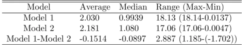
Model Average Median Range (Max-Min) Model 1 2.030 0.9939 18.13 (18.14-0.0137) Model 2 2.181 1.080 17.06 (17.06-0.0047) Model 1-Model 2 -0.1514 -0.0897 2.887 (1.185-(-1.702))

Table 1. Error Statistics.

Parameter Meaning

r1 Maximum proliferation rate of BCR-ABL D population

r2 Maximum proliferation rate of BCR-ABL I population

r3 Maximum proliferation rate of Normal population

p3 Parameter that simulates the crowding effect

n Hill coefficient

q1 Minimum BCR-ABL D cell quota

q2 Minimum BCR-ABL I cell quota

k1 Maximum BCR-ABL D to BCR-ABL I mutation rate

k2 Maximum BCR-ABL I to BCR-ABL D mutation rate

K1 BCR-ABL D to BCR-ABL I mutation half-saturation level

K2 BCR-ABL I to BCR-ABL D mutation half-saturation level

qm1 Maximum BCR-ABL cell quota

vm Cell quota production rate

b Cell quota degradation rate

µm Rate at which BCR-ABL is used within the cell for growth Table 2. Model 1 Parameter Meanings. BCR-ABL D refers to BCR-ABL dependent and BCR-ABL I refers to BCR-ABL inde-pendent.

7. A comparison of the two models.

7.1. Simulations. To compare the two models we ran simulations with MATLAB using the clinical data of the 40 patients from the earlier study [14]. We used the MATLAB built-in function fminsearch to find the optimum parameters for each model for each patient. We calculated the error using the following equation:

error2=

P

i(yi−yiˆ)

2

N (11)

whereN represents the total number of data points,yirepresents the actual value, and ˆyi represents the estimated value from the models.

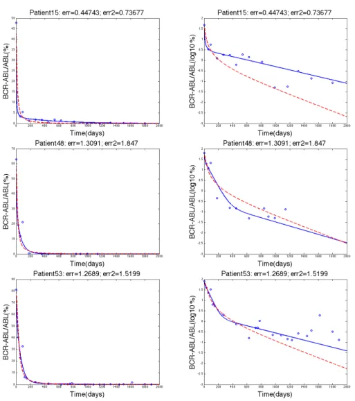
After comparing the errors for each patient from each of the models, 26 out of 40 patients had a smaller error associated with Model 1 compared to Model 2. Table 1 contains statistical information about the errors of the two models. The median error for Model 1 was 0.9939 whereas the median error for Model 2 was 1.080. The average error for Model 1 was 2.030 whereas the average error for Model 2 was 2.181. When comparing the difference between the errors for each model for each patient, only 4 patients out of the 40 patients had a difference in error that was greater than 1. Figure 1 contains the simulations for three patients whose Model 1 error was smaller than the Model 2 error. Figure 2 contains the simulations for

Figure 1. The three rows show the data fitting for patients 15, 48, and 53 respectively where the blue solid line represents Model 1, the dashed red line represents Model 2, and the blue circles represent the clinical data. The left column and the right column both show the same data fitting. The left column has a y-axis of BCR-ABL/ABL(%) whereas the right column have y-axis as log₁₀(BCR-ABL/ABL(%)) values.

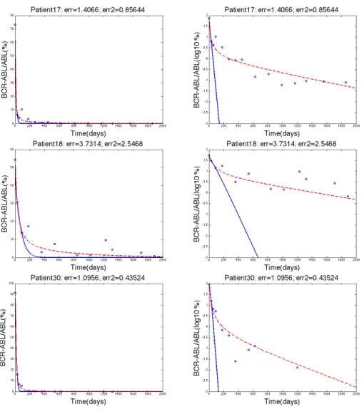
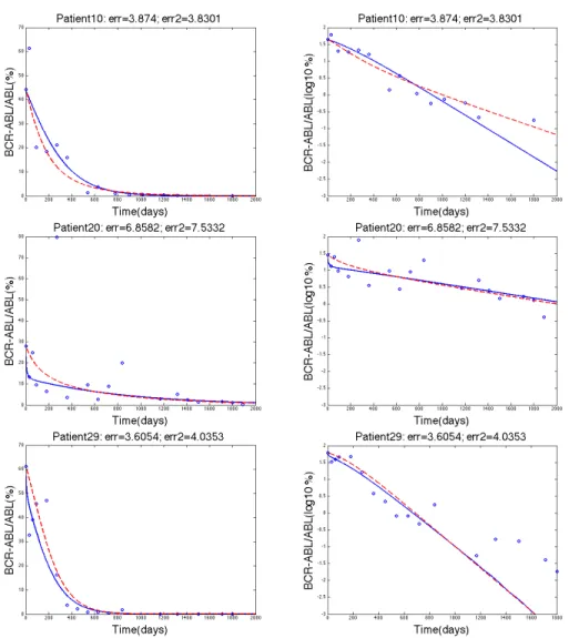
three patients whose Model 2 error was smaller than the Model 1 error. Figure 3 contains the simulations for three patients where the two models were similar in terms of error.

Figure 2. The three rows show the data fitting for patients 17, 18, and 30 respectively where the blue solid line represents Model 1, the dashed red line represents Model 2, and the blue circles represent the clinical data. The left column and the right column both show the same data fitting. The left column has a y-axis of BCR-ABL/ABL(%) whereas the right column have y-axis as log₁₀(BCR-ABL/ABL(%)) values.

7.2. Parameters. Tables 2 and 4 contain the parameter meanings for Model 1 and Model 2 respectively. Tables 3 and 5 contain statistical information about the parameters for the 40 patients for Model 1 and Model 2 respectively. We used the fminsearch function in Matlab to find optimal model parameters with respect to the error defined in (11). The initial guesses for the parameters of the models were initially fit by hand to provide good qualitative agreement with the clinical CML data. Note that both models use the stem cell death rate, d0 = 0.003/day [13]. We can see that, although Model 2 has fewer parameters, the range of the values is

Figure 3. The three rows show the data fitting for patients 10, 20, and 29 respectively where the blue solid line represents Model 1, the dashed red line represents Model 2, and the blue circles represent the clinical data. The left column and the right column both show the same data fitting. The left column has a y-axis of BCR-ABL/ABL(%) whereas the right column have y-axis as log₁₀(BCR-ABL/ABL(%)) values.

extremely large and biologically unrealistic. The maximum value forr3 in Model 1 is about 0.015 per day, whereas the maximum dividing rate for normal stem cells in Model 2 is 6.518×109 per day. The average value for r3 in Model 1 is 0.0061 per day whereas the average value for rx in Model 2 is about 2.341×108 per day. Previous literature [4] have used the value of 0.005 per day to represent the growth rate of normal stem cells, which is much closer to the maximum and average values for Model 1. Although the averages and ranges are very different for the normal stem cell division rate for the two models, the median values are close. The median

Parameter Average Median Range (Max-Min)

r1 0.0054 0.0036 0.021 (0.021-2.713E-11)

r2 0.0225 0.0235 0.042 (0.042-2.587E-4)

r3 0.0061 0.0053 0.015 (0.015-4.919E-8)

p3 1.208E-6 9.454E-7 3.559E-6 (3.563E-6-4.145E-9)

n 2.363 2.050 6.138 (6.238-0.099) q1 0.2854 0.3210 1.011 (1.011-1.722E-8) q2 0.2149 0.2302 0.674 (0.675-2.704E-4) k1 0.0001 0.0001 0.001 (0.001-3.973E-5) k2 0.0001 0.0001 2.091E-04 (2.132E-4-4.132E-6) K1 0.0730 0.0753 0.151 (0.162-0.011) K2 1.6722 1.772 4.025 (4.300-0.275) qm1 5.0489 4.993 14.42 (14.42-0.005)

vm 6.5600E-4 2.879E-4 0.0101 (0.0101-1.3886E-11)

b 0.1469 0.1143 0.470 (0.474-0.004)

µm 0.0125 0.0127 0.061 (0.061-2.058E-8) Table 3. Model 1 Parameter Statistics

Parameter Meaning

ry Maximum dividing rate of leukemic stem cells

rx Maximum dividing rate of normal stem cells

cy Parameter that simulates the crowding effect

cx Parameter that simulates the crowding effect

Table 4. Model 2 Parameter Meanings

value forr3 in Model 1 is about 0.005 while the median value forrx in Model 2 is

about 0.048. Both the median value ofrxin Model 2 and the median value for r3 in Model 1 are essentially the same as the values found in literature.

In Model 1, the growth rate of the nonresistant leukemic stem cells has a maxi-mum value of about 0.021 per day, which is relatively close to the value of 0.008 per day used by Michor [13]. However, the maximum value of ry in Model 2 is about 4.392×107 _{per day, which is biologically unrealistic. For Model 1, the median} and average values forr1 are 0.0036 and 0.0054 respectively, while the median and average values forry in Model 2 are 0.011 and 1.738×106 _{respectively. Although} Model 2 seems to be a much simpler model and fit the data similarly to Model 1, we can see that the parameter ranges are biologically unrealistic, suggesting that Model 1 to be biologically more plausible.

7.3. Resistance. Some patients exhibit a triphasic profile where there is an in-crease in BCR-ABL/ABL% values after the decline. This inin-crease is most likely due to resistance to Imatinib. Although both models were able to show resistance for at least one patient, the resistance described by Model 1 seems more biolog-ically relevant. The BCR-ABL dependent population in Model 1 represents the non-resistant cells while the BCR-ABL independent population represents the re-sistant cells. Model 1 suggests that a relapse occurs when the BCR-ABL dependent

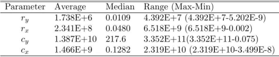
Parameter Average Median Range (Max-Min)

ry 1.738E+6 0.0109 4.392E+7 (4.392E+7-5.202E-9)

rx 2.341E+8 0.0480 6.518E+9 (6.518E+9-0.002) cy 1.387E+10 217.6 3.352E+11(3.352E+11-0.075) cx 1.466E+9 0.1282 2.319E+10 (2.319E+10-3.499E-8)

Table 5. Model 2 Parameter Statistics

population is replaced by the BCR-ABL independent population. Abbott and Mi-chor describe a slightly more complex model [1], which also describes resistance, however the model was not available nor completely described in the paper, so we were not able to compare Model 1 to their model with resistance.

Models that describe resistance are important biologically since resistance is a common problem in cancer treatments. A model by Foo et. al predicted that, for every 100 patients treated with only imatinib, 89 will eventually develop resistance [4]. Models can be used to determine when the patient will stop responding to treat-ment based on their previous data. For chronic phase patients who start imatinib treatment early, only 12% develop resistance within the first two years of treatment [13]. This implies that resistance is probably not an immediate occurrence.

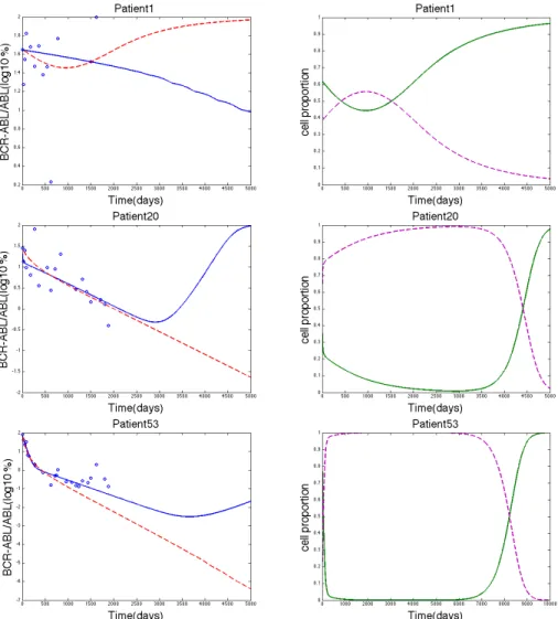
We searched for signatures of resistance using the parameters estimated from patient data. Although clinical data only contains values up to about 5.5 years, we ran the simulations for a longer time span to compare the ability of Model 1 and Model 2 to predict long-term resistance. The simulation for patient 1 in Model 2 showed an increase in BCR-ABL/ABL% around day 1000 (Figure 4), suggesting that the CML cell population started to outgrow the normal cell population. This increase in the leukemia cell population was then verified by the simulation using Model 2 for the proportion of the cell populations (Figure 4). However, patient 1 had the largest error out of all of the other patients for both models. The error for patient 1 from Model 1 was 18.14 and the error from Model 2 was 17.06. The next largest error out of all the patients for Model 1 was 6.858 and for Model 2 was 7.533, which are relatively small errors (errors for patient 20). Thus, neither model accurately describes the patient 1 data, so it seems irrelevant that Model 2 describes resistance for patient 1. Figure 4 also contains graphs where resistance was predicted by Model 1 by an increase in BCR-ABL/ABL%, an increase in the proportion of CML cells, and a decrease in the proportion of normal cells. The errors for these patients were relatively smaller than the errors for patient 1. 8. Discussion. The two models compared in this paper both describe the treat-ment of chronic myeloid leukemia but do so in different ways. Model 2 describes the competition of leukemic and normal stem cells. In Model 1, normal stem cells are in competition with leukemic cells and the growth of leukemic cells depends on the concentration of BCR-ABL. Model 1 also incorporates more biological detail than Model 2 by describing the subcellular dynamics of BCR-ABL and allowing for phenotypic switching between BCR-ABL dependent and independent leukemic cell populations. We compared these two models using clinical data and simulations in order to gain insights into how adding these biological details can more accurately describe and predict resistance to imatinib treatment for CML patients. We found that although Model 2 is a much simpler model, it still describes the data well for

Figure 4. The three rows show simulations for patients 1, 20, and 53 respectively. The left column shows the data fitting for each patient with the y-axis as log₁₀(BCR-ABL/ABL(%)) values, where the blue solid line represents Model 1, the dashed red line represents Model 2, and the blue circles represent the clinical data. The right column shows the proportion of the cell populations, where the green solid line represents the leukemic cells and the dashed purple line represents the normal cells. The model that showed resistance in the left column was used in the simulation for the right column. Model 1 was used for the simulation of the proportion of cells for patients 20 and 53 and Model 2 was used for the simulation of the proportion of cells for patient 1.

some patients. However, the parameter ranges for Model 2 are extremely large and biologically unrealistic. In contrast, Model 1 fit the clinical data better for more patients (26/40) and the estimated parameter ranges were more realistic. This re-sult suggests that the additional biological mechanisms described in Model 1 are relevant, since they can increase the accuracy in data fitting in a majority of patient data.

A mathematical model that predicts treatment resistance in cancer can be a valuable tool to increase the effectiveness of treatment strategies. This is especially relevant for CML where 62% of accelerated phase patients treated with imatinib develop resistance within 2 years of treatment [2]. Using simulations with parameter estimates from patient data, Model 1 was able to predict resistance to imatinib in terms of both an increase in BCR-ABL/ABL% and in the proportion of leukemic cells in the total stem cell population. Model 2 predicted resistance in a single patient, however, the error associated with Model 2 for this patient was relatively large (2.265 times greater than any other patient). Since Model 2 is unable to accurately fit the clinical data for this patient, it is unlikely that the consequent prediction of resistance is accurate. Thus, Model 1 was able to show resistance in some patients in a biologically meaningful way whereas Model 2 was not able to show resistance and accurately model the clinical data.

The results we have discussed for Model 1, although promising, are mainly com-putational and in need of further exploration. A thorough mathematical analysis of Model 1 can provide additional insights into how the subcellular regulation of BCR-ABL levels dictates the long-term transition of CML cells to an imatinib re-sistant phenotype, i.e. BCR-ABL independent. In future computational work we can further evaluate the accuracy of Model 1 to predict resistance by using patient data that exhibits long-term (i.e. >2 years) resistance to imatinib. For example, the simulations for Model 1 where resistance occurs suggest that a more optimal patient data set for evaluating the accuracy of Model 1 is on the time scale of 5-10 years post-treatment initiation.

A novel mechanism encoded in Model 1 is the BCR-ABL dependent switching between BCR-ABL dependent and independent populations. We speculate that these transitions could have an epigenetic basis. This is in contrast to previous CML models that have only considered transitions due to genetic mutations [1] or switching between a proliferative and non-proliferative state [17, 10]. Indeed, re-cent studies have elucidated important epigenetic changes that may cause resistance to the imatinib drug. For example, imatinib therapy could cause drug resistance by affecting epigenetic alterations in cells that down-regulates tumor suppressor genes [15]. Such alterations could lead to a reduced dependence of leukemic cells on BCR-ABL to express a malignant phenotype, i.e. a BCR-ABL independent cell population. Another study showed that aberrant changes in DNA methyla-tion could be an epigenetic marker associated with imatinib resistance [8]. Our computational work here highlights the importance of further experimental work to ascertain the rate at which epigenetic transitions occur in CML, how this rate is related to imatinib dosage, and how it affects imatinib resistance.

Kareva, Berezovskaya, and Castillo-Chavez [9] analyze the balance between im-mature and im-mature myeloid cells and how this balance effects tumors. They claim that if there is a small enough population of cancer cells, then there is a small re-gion of initial conditions where the immune system alone will cure the cancer and the patient will not need treatment. Future work could look into incorporating

the mature and immature myeloid cell populations into the normal cell population in Model 1 as well as combining intermittent imatinib therapy with the immune system’s defense. The work can also be expanded in the future by using more bi-ologically relevant function forms of p(x) and mortality, considering two cell quota variables, and also comparing Model 1 to the model by Roeder et al. [17].

Acknowledgments. We thank Dr. Ingo Roeder for providing the data and the referee for many helpful suggestions. The work of Rebecca A. Everett, Yuqin Zhao and Yang Kuang is supported in part by NSF DMS-0920744.

REFERENCES

[1] L. H. Abbott and F. Michor,Mathematical models of targeted cancer therapy, British Journal of Cancer,95(2006), 1136–1141.

[2] S. Brandford, Z. Rudzki, A. Grigg, J. F. Seymour, K. Taylor, R. Herrmann, C. Arthur, J. Szer and K. Lynch, The incidence of BCR-ABL kinase mutations in chronic myeloid leukemia patients is as high in the second year of imatinib therapy as the first but survival after mutation detection is significantly longer for patients with mutations detected in the second year of therapy,BLOOD,102(2003), 414A.

[3] M. D. Charles and L. Sawyers, Chronic myeloid leukemia, The New England Journal of Medicine,340(1999), 1330–1340.

[4] J. Foo, M. W. Drummond, B. Clarkson, T. Holyoake and F. Michor,Eradication of chronic myeloid leukemia stem cells: A novel mathematical model predicts no therapeutic benefit of adding G-CSF to imatinib, PLoS Computational Biology,5(2009), 1–11.

[5] D. Frame, Chronic myeloid leukemia: Standard treatment options, American Journal of Health-System Pharmacy,63(2006), S10–S14.

[6] M. E. Gorre, M. Mohammed, K. Ellwood, N. Hsu, R. Paquette, P. Nagesh Rao and C. L. Sawyers,Clinical resistance to STI-571 cancer therapy caused by BCR-ABL gene mutation or amplification,Science,293(2001), 876–880.

[7] I. J. Griswold, M. MacPartline, T. Bumm, V. L. Goss, T. O’Hare, K. A. Lee, A. S. Corbin, E. P. Stoffregen, C. Smith, K. Johnson, E. M. Moseson, L. J. Wood, R. D. Polakiewicz, B. J. Druker and M. W. Deininger,Kinase domain mutants of bcr-abl exhibit altered transforma-tion potency, kinase activity, and substrate utilizatransforma-tion, irrespective of sensitivity to imatinib, Molecular and Cellular Biology,26(2006), 6082–6093.

[8] J. Jelinek, V. Gharibyan, M. Estecio, K. Kondo, R. He, W. Chung, Y. Lu, N. Zhang, S. Liang, H. Kantarjian, J. Cortes and J-P. Issa,Aberrant DNA methylation is associated with disease progression, resistance to imatinib and shortened survival in chronic myelogenous leukemia, PLoS ONE,6(2011), e22110.

[9] I. Kareva, F. Berezovskaya and C. Castillo-Chavez,Myeloid cells in tumour-immune inter-actions, Journal of Biological Dynamics,4(2010), 315–327.

[10] N. L. Komarova and D. Wodarz,Effect of cellular quiescence on the success of targeted CML therapy, PLoS ONE,2(2007), e990.

[11] F. Michor,Reply: The long-term response to imatinib treatment of CML, Biritish Journal of Cancer,96(2007), 697–680.

[12] F. Michor,Quantitative approaches to analyzing imatinib-treated chronic myeloid leukemia, TRENDS in Pharmacological Sciences,28(2007), 197–199.

[13] F. Michor, T. P. Hughes, Y. Iwasa, S. Branford, N. P. Shah, C. L. Sawyers and M. A. Nowak, Dynamics of chronic myeloid leukemia, Nature,435(2005), 1267–1270.

[14] M. C. Muller, N. Gattermann, T. Lahaye, M. W. N. Deininger, A. Berndt, S. Fruehauf, A. Neubauer, T. Fischer, D. K. Hossfeld, F. Schneller, S. W. Krause, C. Nerl, H. G. Sayer, O. G. Ottmann, C. Waller, W. Aulitzky, P. le Coutre, M. Freund, K. Merx, P. Paschka, H. Konig, S. Kreil, U. Berger, H. Gschaidmeier, R. Hehlmann and A. Hochhaus,Dynamics of BCR-ABL mRNA expression in first-line therapy of chronic myelogenous leukemia patients with imatinib or interferon a/ara-C, Leukemia,17(2003), 2392–2400.

[15] C. Nishioka, T. Ikezoe, K. Udaka and A. Yokoyama,Imatinib causes epigenetic alterations of PTEN gene via upregulation of DNA methyltransferases and polycomb group proteins, Blood Cancer Journal,1(2011), e48.

[16] T. Portz, Y. Kuang and J. D. Nagy,A clinical data validated mathematical model of prostate cancer growth under intermittent androgen suppression therapy, AIP Advances,2(2012), 011002.

[17] I. Roeder, M. Horn, I. Glauche, A. Hochhaus, M. C Mueller and M. Loeffler,Dynamic mod-eling of imatinib-treated chronic myeloid leukemia: Functional insights and clinical implica-tions, Nature Medicine,12(2006), 1181–1184.

[18] A. M. Stein, D. Bottino, V. Modur, S. Branford, J. Kaeda, J. M. Goldman, T. P. Hughes, J. P. Radich and A. Hochhaus,BCR-ABL transcript dynamics support the hypothesis that leukemic stem cells are reduced during imatinib treatment, Clinical Cancer Research, 17 (2011), 6812–6821.

Received October 10, 2012; Accepted January 28, 2013.

E-mail address:[email protected] E-mail address:[email protected] E-mail address:[email protected] E-mail address:[email protected]