Vulnerability Analysis
Erik Jenelius
Doctoral Thesis in Infrastructure
with specialisation in Transport and Location Analysis October 2010
Division of Transport and Location Analysis Department of Transport Science KTH Royal Institute of Technology
ISSN 1653–4468
ISBN 978–91–85539–63–5
Akademisk avhandling som med tillst˚and av Kungliga Tekniska H¨ogskolan i Stockholm framl¨agges till offentlig granskning f¨or avl¨aggande av teknologie doktorsexamen tisdagen den 19 oktober 2010 kl 13.00 i sal D3, Lindstedtsv¨agen 5, Kungliga Tekniska H¨ogskolan, Stockholm.
www.infra.kth.se/~jenelius/ © Erik Jenelius 2010
of Transport Science, KTH, Stockholm. ISBN 978–91–85539–63–5.
Abstract
Disruptions in the transport system can have severe impacts for affected individu-als, businesses and the society as a whole. In this research, vulnerability is seen as the risk of unplanned system disruptions, with a focus on large, rare events. Vulnerability analysis aims to provide decision support regarding preventive and restorative actions, ideally as an integrated part of the planning process.
The thesis specifically develops the methodology for vulnerability analysis of road networks and considers the effects of suddenly increased travel times and can-celled trips following road link closures. The major part consists of model-based studies of different aspects of vulnerability, in particular the dichotomy of system efficiency and user equity, applied to the Swedish road network. We introduce the concepts of link importance as the overall impact of closing a particular link, and regional exposure as the impact for individuals in a particular region of, e.g., a worst-case or an average-case scenario (Paper I). By construction, a link is im-portant if the normal flow across it is high and/or the alternatives to this link are considerably worse, while a traveller is exposed if a link closure along her normal route is likely and/or the best alternative is considerably worse. Using regression analysis we show that these relationships can be generalized to municipalities and counties, so that geographical variations in vulnerability can be explained by vari-ations in network density and travel patterns (Paper II). The relvari-ationship between overall impacts and user disparities are also analyzed for single link closures and is found to be negative, i.e., the most important links also have the most equal distribution of impacts among individuals (Paper III).
In addition to links’ roles for transport efficiency, the thesis considers their im-portance as rerouting alternatives when other links are disrupted (Paper IV). Such redundancy-important roads, found often to be running in parallel to highways with heavy traffic, may be warranted a higher standard than their typical use would suggest. We also study the vulnerability of the road network under area-covering disruptions, representing for example flooding, heavy snowfall or forest fires (Pa-per V). In contrast to single link failures, the impacts of this kind of events are largely determined by the population concentration, more precisely the travel de-mand within, in and out of the disrupted area itself, while the density of the road network is of small influence. Finally, the thesis approaches the issue of how to value the delays that are incurred by network disruptions and, using an activity-based modelling approach, we illustrate that these delay costs may be considerably higher than the ordinary value of time, in particular during the first few days after the event when travel conditions are uncertain (Paper VI).
This thesis would not have seen the light of day without the collaboration, support and encouragement from a large number of people. First and foremost I wish to thank my supervisor Professor Lars-G¨oran Mattsson and assistant supervisor Dr. Katja Vourenmaa Berdica. Lars-G¨oran’s ability to discern good ideas from bad and to balance theoretical soundness with practical applicability has been invaluable, not to mention his excitement for the subject. Katja, my “predecessor”, did the hard but seminal work of framing the field of road network vulnerability, which has made my own work so much easier. She has also contributed with ideas and encouragement throughout the project. Special thanks go also to my co-author Tom Petersen, whom I much enjoyed working with.
I wish to thank everybody at the Division of Transport and Location Analysis who have been very inspiring and supporting company these years. I take the
op-portunity to thank in particular Professor Torbj¨orn Thed´een and Dr. ˚Ake J.
Holm-gren at the Centre for Safety Research who supervised my Master’s Thesis and have continued to back me during this time. Special thanks also to Jonas Westin, unfortunately there was no room for our joint work in this thesis.
I wish to thank Professor David Levinson at the University of Minnesota and his research group for generously welcoming me to spend the summer of 2009 with them and providing valuable ideas, feedback and access to data.
The reference group for the project “Vulnerability analyses of road networks” has shown great interest in my work and has provided many good ideas and
sug-gestions. Hence, I want to thank all its past members: ¨Orjan Asplund, Jan Bergl¨of,
Fredrik Brandt, Per J. Eriksson, Johan Hansen, Per Lindroth, Peter Rehnman, Leif Ringhagen, Kenneth W˚ahlberg and Mulugeta Yilma. I am also grateful to Profes-sor Lars Westin, Ume˚a University, for giving helpful feedback on the thesis as a whole at the pre-defense seminar in June this year.
The financial support from the Swedish Road Administration (V¨agverket), the Swedish Governmental Agency for Innovation Systems (VINNOVA), and the Swe-dish Research Council for Environment, Agricultural Sciences and Spatial Plan-ning (FORMAS) that made this work possible is gratefully acknowledged.
Finally, I would like to express my gratitude to my friends and family for being a constant support, so easily taken for granted, along every small step leading to this thesis.
Stockholm, September 2010 Erik Jenelius
I Jenelius, E., Petersen, T. and Mattsson, L.-G. (2006) Importance and exposure
in road network vulnerability analysis.Transportation Research Part A: Policy
and Practice40(7), 537–560.
II Jenelius, E. (2009) Network structure and travel patterns: Explaining the
geo-graphical disparities of road network vulnerability. Journal of Transport
Ge-ography17(3), 234–244.
III Jenelius, E. (2010a) User inequity implications of road network vulnerability.
Journal of Transport and Land Use2(3/4), 57–73.
IV Jenelius, E. (2010b) Redundancy importance: Links as rerouting alternatives
during road network disruptions. Procedia Engineering3, International
Con-ference on Evacuation Modelling and Management, 129–137.
V Jenelius, E. and Mattsson, L.-G. (2010) Road network vulnerability analysis of area-covering disruptions: A grid-based approach with case study. Submitted. VI Jenelius, E., Mattsson, L.-G. and Levinson, D. (2010) The traveler costs of
un-planned transport network disruptions: An activity-based modeling approach. Submitted.
1 Introduction . . . 1
2 Vulnerability, risk and reliability . . . 2
3 Experiences from road network disruptions . . . 4
3.1 The I-35W bridge collapse, Minneapolis, 2007 . . . 4
3.2 The flash flood at ˚Ann, Sweden, 2006 . . . 5
3.3 Disruption causes and impacts . . . 6
4 Quantitative vulnerability analysis: A review. . . 8
5 Perspectives of vulnerability analysis . . . 11
5.1 Importance and criticality . . . 11
5.2 Vulnerability and exposure . . . 13
6 A formal framework for vulnerability measures . . . 14
6.1 User exposure . . . 16
6.2 Aggregate group exposure . . . 17
6.3 Element importance . . . 18
7 From formal to practical measures . . . 18
8 Importance and exposure measures in the thesis . . . 21
8.1 Importance measures . . . 21
8.2 Exposure measures . . . 22
9 Vulnerability and its determinants: Some general results . . . 23
9.1 Data and models . . . 24
9.2 Link and cell importance . . . 24
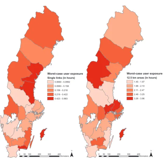
9.3 Worst-case regional user exposure . . . 27
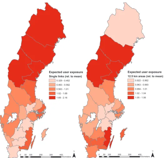
9.4 Expected regional user exposure . . . 28
10 On the delay costs of road network disruptions. . . 30
11 Conclusion and challenges for the future . . . 33
11.1 Vulnerability management . . . 34
11.2 Vulnerability of other transport systems . . . 36
References . . . 37
Our world is dominated by the extreme, the unknown, and the very improbable (improbable according to our current knowledge)—and all the while we spend our time engaged in small talk, focusing on the known, and the repeated.
Nassim Nicholas Taleb,The Black Swan, 2007
1. Introduction
Modern society relies upon the collection of systems and institutions known as the infrastructure to provide comfort and security for the people. Some of these systems are more fundamental than others in the sense that they supply services that other systems require. These most basic systems include housing, water sup-ply, heating, communications and—the focus of the present thesis—various modes of transport. On these more elaborate institutions and services are built, such as health care, law enforcement, waste management, education and finance. There also exist interdependencies between systems, for example electric power and data communications, so that the performance of one system depends on the other and vice versa (e.g., Rinaldi et al., 2001; Little, 2002).
The welfare and living standard of a society is intrinsically linked to the level at which its infrastructure is developed and maintained. A downside of this depen-dency, perhaps almost equally intrinsic, is that sudden failures and disruptions in the systems can cause severe strains on the society. The systems of which degrada-tions would have the largest negative impacts are often collectively referred to as thecritical infrastructure. The constituting systems may vary between countries and the evaluation criteria used, but have invariably included transport systems in general and the road transport system in particular (for USA, see, e.g., Moteff and Parfomak (2004); for Sweden, see KBM (2005)).
We use the term vulnerability analysis to refer to the study of potential degrada-tions of the infrastructure and their impacts on society. Infrastructure vulnerability
is thus the extent to which infrastructure disruptions lead to reductions in the
wel-fare of the society, or simply put, theriskof infrastructure disruptions; see further
Section 2. This thesis focuses on the road transport system, more specifically on
disruptions of components in the road network (roads and intersections). Road
network vulnerability analysisis thus a special case of infrastructure vulnerability analysis, which suggests that many concepts and approaches found in the broader field are relevant here, and vice versa. At the same time, each infrastructure system has its own inherent purposes and characteristics that need to be taken into account in a vulnerability analysis. This thesis contributes concepts and perspectives that are generally applicable and useful in infrastructure vulnerability analysis, as well as metrics, models and analyses that are specific to the road transport system.
2. Vulnerability, risk and reliability
The word vulnerability is used in every-day language to express a sensitivity to at-tack or injury. As is often the case with popular terms, there is no generally adopted notion of what road transport or infrastructure vulnerability is. For example, Willis (2007) focuses on the ability to withstand an attack and defines vulnerability as the probability that an attack results in damage, given that an attack occurs. Tay-lor et al. (2006) defines a node in a road network to be vulnerable “if loss (or substantial degradation) of a small number of links significantly diminishes the accessibility of the node, as measured by a standard index of accessibility”. Thus, whereas some authors stress the probability of negative consequences, others stress the magnitude of the negative consequences. Still other views are proposed by, e.g., Einarsson and Rausand (1998), Haimes (2006), Aven (2007), Ezell (2007) and Jo-hansson (2010). We shall not attempt a full literature review of the vulnerability concept here; a further discussion is found in Paper I.
In this thesis we propose that vulnerability is risk, where our notion of risk
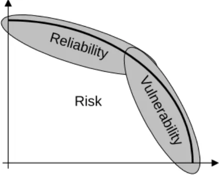
is adopted from Kaplan and Garrick (1981), with a focus on a particular kind of scenarios. According to those authors, a risk analysis consists of answering three questions: (i) What can happen? (ii) How likely is it that that will happen? and (iii) If it does happen, what are the consequences? The results of the analysis can thus be represented as a list of “triplets”, each consisting of a description of a particular scenario, the probability of that scenario occurring, and the impact of the scenario. The risk is then the set of all triplets. If the impact of each scenario is expressed as a single number, sorting the scenarios according to increasing impacts and plotting the probability that the impact is larger than a given value gives a representation of the risk known as the “risk curve”; see Figure 1 for an illustration.
In our view, then, infrastructure vulnerability is society’s risk of infrastructure system disruptions and degradations. Based on the general definition of risk from Kaplan and Garrick (1981), we have thus defined the target for which the impacts
Reliability V u lne rab ility Impact Probability Risk
Figure 1: Illustration of the relationships between road transport system disruption risk, vulnerability and reliability as perceived in this thesis. The thick line represents the “risk curve” of Kaplan and Garrick (1981), i.e., the probability that the impact is greater or equal to a given value.
are to be assessed (although very generally), i.e., the society. We have also put restrictions on the kind of scenarios that we consider, i.e., infrastructure system
disruptions. However, there is another widely used concept, reliability, that can
be said to fit into roughly the same definition, and we want to make a distinction between vulnerability and non-reliability.
In the quantitative risk analysis literature, reliability is defined quite strictly as “the probability of a device performing its purpose adequately for the period of time intended under the operating conditions encountered” (Høyland and Rausand, 1994). Reliability analysis generally models systems as being structures of com-ponents, each with a certain stochastic life length. The purpose of the analysis is typically to calculate the expected life length of the system, or if components are repaired, the probability that the system is operational at a given time. From this perspective, reliability analysis thus represents a different restriction of risk analy-sis than vulnerability analyanaly-sis, in which the impacts of scenarios are only evaluated as whether a system is performing its purpose adequately or not (e.g., a machine or a plant manufacturing goods according to set quality standards).
The term reliability is often also applied less strictly, not least in transport re-search where it may refer to the stability and predictability of travel conditions such as travel times over time (see further Section 4). When used in this sense, relia-bility studies are focused on the upper left corner of Figure 1, that is, the impacts from relatively frequent and moderate fluctuations in travel conditions; typically, it is assumed that users know the probability distribution of travel conditions but not the realised conditions on a given day (e.g., Fosgerau and Karlstr¨om, 2010).
To distinguish vulnerability analysis from reliability analysis, in particular with regard to the road transport system, we will further restrict the focus of vulnera-bility analysis to mainly the lower right corner of Figure 1, that is, relatively rare
events with severe impacts. As Figure 1 also indicates, the two concepts can be considered to be overlapping, and we will not attempt to define, nor do we de-sire, a precise boundary between them. The relationships between the concepts of risk, reliability and vulnerability with respect to the road transport system are also discussed by for example Berdica (2002), Nicholson (2003) and Husdal (2004).
3. Experiences from road network disruptions
Before entering the field of model-based, quantitative vulnerability analysis it is important to consider what can be learnt from empirical observations of real events. To this end, we first consider two recent disruptions of road transport systems, one international with very severe impacts and one Swedish with more moderate impacts for society; it is likely that the reader will know of similar events that have occurred in her own vicinity. We then complement the picture with evidence gathered from other major and minor events.
3.1. The I-35W bridge collapse, Minneapolis, 2007
At approximately 6:05 pm on August 1 2007 the I-35W bridge in Minneapolis, Minnesota collapsed without warning into the Mississippi river. In its accident re-port, the National Transportation Safety Board (NTSB) identified a design flaw, in combination with ongoing repair work that put an unusually heavy load on the structure, as the likely cause of the failure. The collapse had immediate and tragic effects since thirteen people were killed and 145 people were injured (NTSB, 2008).
As the bridge carried a typical flow of 140,000 vehicles per day, the collapse meant a significant disruption of normal travel conditions. Surveys and loop detec-tor data showed that it took several weeks for the traffic to settle into a new stable state and that people responded primarily by changing routes, departure times and destinations and possibly by consolidating trips. Public transport services expe-rienced an increase in ridership during the disruption, but as the modal share of public transport is low in the area the effect on car traffic was limited (Zhu et al., 2010b).
A number of adjustments of the transport infrastructure were made within days after the collapse in order to better accommodate the increased traffic flows in the surrounding network. This included transforming a bus-only shoulder lane to a fourth normal lane on the parallel I-94 bridge and blocking certain on- and off-ramps. On September 18 2008 a replacement bridge was opened, while the fourth lane on the I-94 bridge was removed on October 12. Surveys and detector data show that the traffic adapted more quickly to the reopening, which was well known beforehand, than to the collapse. Somewhat paradoxically, the overall benefits
on travel times from the opening of the new bridge were more than offset by the restoration of the fourth I-94 lane to a shoulder lane (Zhu et al., 2010a).
The total societal costs of the bridge collapse are difficult to survey. On August 6 2007 the state of Minnesota was granted 250 million USD in federal emergency relief funding for clean-up, recovery and restoration (Horwath, 2007). The con-struction of the new bridge cost approximately 234 million USD (Lohn, 2007), while victims of the collapse were compensated by the state of Minnesota with in total 38 million USD (Lohn, 2008). Further cost components for which we have not found estimates include the emergency rescue and recovery efforts, the clean-up of water and land, and the modifications of the road infrastructure other than building the new bridge.
Soon after the collapse an assessment of the costs due to delays was made. Changes in travel time were calculated using a transport planning model system, which were then multiplied with a composite car and truck value of time of 14.19 USD/hour to obtain the delay costs. These were estimated to between 71 thousand USD and 220 thousand USD per day depending on assumptions about traveller response (Xie and Levinson, 2009). In a separate assessment the Minnesota De-partment of Transport estimated the traveller costs to 400 thousand USD per day, including increases in both travel time and distance. The total impacts on Min-nesota’s economy were estimated to 17 million USD in 2007 and 43 million USD in 2008 (State of Minnesota, 2008).
3.2. The flash flood at ˚Ann, Sweden, 2006
At around 6:45 pm on July 30 2006 the E14 European highway between
Trond-heim, Norway and Sundsvall, Sweden, was cut off west of ¨Ostersund on the
Swe-dish side of the border. Heavy cloudbursts during the day had caused the flooding of a small stream, which eroded the ground upstream of the road. The water carried large quantities of soil, trees and debris toward the road, causing the insufficiently dimensioned road drains to choke up. Within a few hours, the pool of water that formed at the mouth of the drains caused the road structure to collapse and about 30 meters of the road was completely washed away. A railway going along the down-stream side of the road was also demolished by the unleashed flood (L¨anstidningen
¨
Ostersund, 2006b).
The road is an important connection between Sweden and Norway with a daily flow of about 1000–2000 vehicles, and long queues were built up before traffic was redirected along alternative routes. People living on one side of the incident area and working on the other were forced to make a daily detour of more than 200 kilo-meters. Tracked vehicles were called in to transport people past the area. Swedish residents living west of the area were unable to reach medical care in Sweden and were referred to Norway. After two days a small temporary parallel road was built next to the incident area. The road only allowed vehicles to pass in one direction
at a time, and could only carry vehicles without trailers and weights below four tonnes. Ambulances were now able to reach people beyond the area (J¨amtlands
l¨ans landsting, 2006; L¨anstidningen ¨Ostersund, 2006a,d; V¨agverket, 2006a).
On August 11, twelve days after the event, the E14 was reopened after repairs. Initially, one lane was kept closed and the speed limit of the road was reduced because of ongoing work. The old drain pipes were replaced with new pipes with a larger dimension to reduce the risk of similar events occurring again. The cost of the repairs was estimated to about eight million SEK (about 1.2 million USD) for the road and a similar amount for the railway. The regional train operator estimated that loss of revenues, substitution of traffic with bus and taxi, repair costs for a damaged train and bad-will effects led to a cost of 1.5 million SEK. No calculation of the societal costs due to increased travel times appears to have been presented
(L¨anstidningen ¨Ostersund, 2006c; L¨anstrafiken i J¨amtlands L¨an, 2007; V¨agverket,
2006b; V¨agverket Produktion, 2006). 3.3. Disruption causes and impacts
Many types of scenarios can potentially cause severe disturbances in the road trans-port system. To begin with, some events are caused by the traffic itself, in the form of car accidents or exceptional congestion due to large public events. Some incidents are caused by external accidents such as industrial leakages or ships ram-ming bridges (e.g., the ramram-ming of Essingeleden in Stockholm, Sweden, October 14 2005); others are caused by technical failures of the road structure, bridges, etc., due to wear and tear or faulty construction (e.g., the I-35W bridge collapse described above). Still others are caused by adverse meteorological, hydrolog-ical or geologhydrolog-ical conditions, such as flash floods, snow storms, landslides and earthquakes, that either disrupt the road network or obstruct the traffic (e.g., the Northridge earthquake 1994). Furthermore, we cannot ignore the reality of inten-tional attacks on the transport system, for example as a means to inflict disorder and panic to the society or to delay the police after a robbery (e.g., the train bombings in Madrid 2004).
Berdica (2000) studies the most common causes of complete road closures in the Swedish road network, which are found to be, in descending order, road works, floods, traffic accidents, snow, storm-related incidents, hazardous goods accidents, physical collapses, thaw weakening damage, and bridge openings.
Just like the causes, the effects of road network disruptions can be multifaceted. First and most severely, some events, for instance car accidents and infrastructural collapses, may cause injuries and fatalities directly. There may also be service disturbances that will threaten life and health indirectly. One such service is the ability for people to receive emergency medical care. In a worst-case scenario an incident may cut off all possibilites to reach a hospital or for an ambulance to reach the person in need; in other cases, the alternative routes may be too long.
Assistance from the police and the fire department also belong to this category. Second, there are the less acute consequences, i.e., disturbances that are not a threat to life and health in the short run, but may cause anything from substantial economic and social strains to mere nuisances. For people, this includes impaired abilities to get to work in time, to drop off and pick up children from daycare and school, to do the shopping, to attend leisure activities, and so on. For companies, the impacts include delayed deliveries and supplies (with possible ripple effects), loss of manpower and customers, increased freight costs, delayed or cancelled busi-ness meetings, etc. All these impacts are associated with societal costs, although it may vary from case to case, through insurance, settlements, court rulings etc., which parties actually end up paying for the effects.
Third, there may be large costs associated with remedies and restoration of the transport system to a fully operational state. These costs may range from rel-atively low, for example when towing away crashed vehicles or providing emer-gency rerouting, to very high, such as when rebuilding or replacing a collapsed bridge or road segment.
Regarding the traffic responses to unplanned transport network disruptions, empirical evidence tells us that such events are generally followed by a time—on the order of days or weeks—of uncertainty, learning and adaptation for the trav-elers. If the degradation is long-lasting, the traffic eventually approaches a new equilibrium-like state, where travelers have received sufficient information about the new travel conditions and adjusted their travel decisions accordingly. Obser-vations are fairly consistent in that the most common responses by individuals are changes in departure time and route choice. To a lesser extent people cancel or con-solidate (mainly non-work) trips, whereas people are relatively reluctant to change travel mode (Wesemann et al., 1996; Giuliano and Golob, 1998; Hunt et al., 2002; Cairns et al., 2002; Clegg, 2007; Zhu et al., 2010b).
In many areas, for example in USA (Transportation Research Board, 2008)
and the UK (Department for Transport, 2004),climate change is predicted to
in-crease the strains on the road infrastructure. Recently, a commission investigating the consequences for Sweden of the anticipated climate changes concluded that the risk for floods, landslides and erosion will increase in many areas, affecting houses, railways and roads (Klimat- och s˚arbarhetsutredningen, 2007). For the road net-work the costs associated with these damages between the years 2010 and 2100 are estimated to 10–20 billion SEK (ca. 1.5–3 billion USD). The commission suggests that adaptations of the transport infrastructure to a changed climate should be made a part of the national transport policy goals, and that resources should be earmarked for this purpose. Furthermore, the risks for the road and railway networks should be surveyed and countermeasures taken.
4. Quantitative vulnerability analysis: A review
Traditionally, transport policy and planning has been focused on the performance of the transport system under typical demand and supply conditions. In recent years, however, it has been increasingly recognized that variations from the normal state can cause considerable reductions in efficiency. The ability of the transport system including its users to handle fluctuations in operating conditions has be-come known as transport or travel reliability. Studies in this field usually consider some aspect of the transport system such as link capacities, travel demand or travel times to vary randomly according to some specified distribution and assess the user costs or the impacts on system performance from this variability.
One of the earliest and simplest measures of transport network reliability is terminal or connectivity reliability, which is the probability that there is still a con-nection between a pair of nodes in the network when one or more links are closed (e.g., Wakabayashi and Iida, 1992; Bell and Iida, 1997). More refined reliability measures that have been introduced include travel time reliability, i.e., the proba-bility that a trip can be completed within a specified time interval (e.g., Yang et al., 2000; Clark and Watling, 2005) and capacity reliability, defined as the probabil-ity that a network can accommodate a specified level of travel demand (e.g., Yang et al., 2000; Chen et al., 2002). The travellers’ costs of travel time uncertainty and variability have been studied both theoretically and empirically by for exam-ple Noland and Small (1995), Bates et al. (2001), Noland and Polak (2002) and Fosgerau and Karlstr¨om (2010). For fuller overviews of the subject see Iida and Bell (2003) and Watling (2008).
The field of transport network vulnerability (and robustness, which may be seen as the converse of vulnerability) focuses mainly on larger, unexpected disruptions rather than the day-to-day variability in travel conditions and has received growing attention as well. Early contributions include Garrison (1960) who used graph-theoretical concepts to analyze the structure of the US Interstate Highway system and found that the failure of a link in the network could lead to long detours. In the field of operations research, algorithms for finding the most important (or “vital”) nodes and links in networks were also developed early (e.g., Ratliff et al., 1975; Ball et al., 1989). The goal of these mathematical programs is typically to find the node or link that when removed increases the length of the shortest path or reduces the maximum flow between a given origin node and destination node the most.
The current research interest in transport vulnerability commenced in the early 2000s, largely as part of a broader focus on critical infrastructure protection. Sev-eral recent natural disasters, including the earthquakes in Los Angeles 1994 and Kobe 1995, and terrorist attacks, most prominently the events on September 11 2001, raised awareness that society is vulnerable to disruptions in these infrastruc-ture systems. It was recognized by some researchers that the methods from the transport reliability field were inadequate for assessing the consequences of
se-vere, albeit seemingly unlikely, disruptions of the road transport system and that new approaches were necessary (Berdica, 2002; D’Este and Taylor, 2003; Nichol-son, 2003).
As requested by these authors, the vulnerability research has embraced a rich exploration of approaches, metrics and models. The applied literature can be broadly classified with respect to the kind and range of disruption scenarios that are studied. The following categories are largely based on the overview of the more general field of infrastructure vulnerability analysis given by Murray et al. (2008), who also discuss the benefits and disadvantages of the different approaches in depth.
A first category of studies have focused on one or a few specific scenarios. Notably, several authors have assessed the economic impacts of earthquakes dis-rupting the road network using integrated transport network and multiregional trade models (Cho et al., 2001; Kim et al., 2002; Ham et al., 2005; Tatano and Tsuchiya, 2008). Suarez et al. (2005) study the impacts of flooding and climate change on the urban transport system of Boston Metro Area, USA, using a four-stage (i.e., trip generation, destination choice, mode choice and route choice) transport modeling system. Similar approaches are used by Berdica and Mattsson (2007) to evaluate the societal impacts of bridge closures in Stockholm, Sweden, and Taylor (2008) for a tunnel blockage in Adelaide, Australia.
A second category of studies, descendant from the work of for example Ratliff et al. (1975), use mathematical modeling and optimization techniques to identify worst-case scenarios, or best responses to such scenarios. Matisziw and Murray (2009) use an integer programming formulation to identify the most severe disrup-tions of a given number of links in the truck transport network of Ohio, USA. Bell et al. (2008) integrate a macroscopic traffic assignment model in a game-theoretic framework to determine routing strategies for the shipment of VIPs in London, UK under the risk of antagonistic attacks.
A third category of studies consider a full range of scenarios, through either exhaustive calculation or Monte Carlo simulation. Dalziell and Nicholson (2001) present what may perhaps be called the only complete road network vulnerabil-ity analysis and management study in the literature. In the study, focused on the Central North Island road network of New Zealand, the authors identify a range of plausible disruption hazards (including snow and ice, ash fall, earthquakes and car crashes) along with a frequency distribution of closure durations for each haz-ard. Specific scenarios with different closure durations are then generated through Monte Carlo simulation, and the impacts including both restoration work and the economic losses of the travellers are evaluated. Following this assessment a cost-benefit analysis is performed to identify the most efficient options for mitigating the identified vulnerabilities.
Several authors have performed full range studies of single link failures in road networks. Taylor et al. (2006) analyze the Australian road network at different
levels, using various measures of diminished accessibility to evaluate the impacts of link failures. Sohn (2006) proposes an accessibility index that integrates road distance and traffic volumes and uses it to assess the importance of highway links in Maryland, USA, under flood damage. Knoop et al. (2008) use macroscopic traffic simulation to evaluate the impacts of link blockings in Rotterdam, the Netherlands. In a study of the Swiss road network, Erath et al. (2009) handle the computational challenges associated with full range analyses by restricting the calculations to a subnetwork surrounding each disrupted link. We may note, finally, that Papers I–V in the present thesis also belong to this category.
As Murray et al. (2008) note, the different approaches to vulnerability analysis all have their merits and shortcomings. With a scenario-specific assessment, it is possible to use sophisticated quantitative models that can capture many features of the particular scenario and system. There is a risk, however, that other relevant and possibly more severe scenarios are overlooked, which could lead to a biased picture of the situation. With optimization approaches, it is possible to identify worst-case scenarios, which are undoubtedly of great value, without exhaustive examination of all possible scenarios. Again, there is a danger that other severe scenarios may be overlooked, and also that the properties of the mathematical program to a large extent determines what vulnerability metrics are feasible to use.
Finally, with a full range approach, one gets a comprehensive picture of the vulnerability of the network, including worst-case scenarios as well as distribu-tions across users and regions. It is also possible to draw general conclusions about the factors underlying vulnerability. This comes at the price of extensive calcula-tions, which may require simplified models and vulnerability metrics to be feasible. Such simplifications, in turn, may mean that important features of the system and individual scenarios are overlooked.
In addition to these studies, a number of authors have proposed indices to eval-uate road network vulnerability and quantify link and node importance, although they have only been applied to test networks. Thus, Murray-Tuite and Mahmassani (2004) propose a vulnerability index that accounts for traffic flow, link capacities, travel times and the availability of alternative routes. Scott et al. (2006) propose a Network Robustness Index to identify important links in highway networks, which is defined as the increase in vehicle travel time that is incurred when the link is closed. The index is generalized by Sullivan et al. (2010) who note that complete link closures are only one of many possible kinds of disruption scenarios and argue that the level of capacity reduction should be considered that gives the most stable importance ranking of different links. Another similar importance measure, based on the inverse of travel cost, is defined by Qiang and Nagurney (2008).
Some papers develop and investigate the models that are used to calculate the impacts of network disruptions; Paper VI here belongs to this category. Chen et al. (2007) propose the use of a combined travel demand model incorporating trip gen-eration, destination choice, mode choice, and route choice to assess the long-term
equilibrium effects of a closure of one or more links. The consequences are cal-culated as the decrease of a utility-based accessibility measure. He et al. (2009) model the day-to-day development of traffic flows after unplanned network disrup-tions based on past experiences and beliefs about the future condidisrup-tions. Notably, Berdica et al. (2003) study the consequences of the same incident scenario with three different models (on the macro, meso and microscopic scales, respectively) and find that the results differ significantly. The authors remark that “although a model may be well calibrated for normal conditions, there is no guarantee that it will predict abnormal conditions correctly”.
5. Perspectives of vulnerability analysis
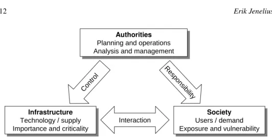
As illustrated in Figure 2 an infrastructure system such as the road transport system can be seen as consisting of three parts: First, there is the technical and physical infrastructure including roads, traffic signals, vehicles etc. Second, there are the direct and indirect users of the technology, i.e., travellers, transporters and society in general. Third, there are the planning and operating authorities responsible for providing and maintaining the technology and the infrastructure in order to serve society under given regulations and budget restrictions. In economic terms the first (technology) and second (users) parts can be regarded as the supply and demand sides of the system, respectively, while the third part (authorities) regulates the two sides and their interactions.
It should be noted that for planning and operating authorities the defined strate-gic goals are typically centered on the users and the society, such as efficiency, ac-cessibility, reliability, safety, equality and regional development. Meanwhile, the available decision variables are mainly concentrated to the technological supply side, including new road projects, maintenance, traffic signal settings, speed limits and road tolls.
5.1. Importance and criticality
This trisecting systems model suggests two main perspectives on vulnerability (or any other issue) from the point of the responsible authorities. The first perspective
focuses on thetechnologicalside of the system. For a given component or group
of components, here collectively called anelement, we may ask: What is the
prob-ability that the element is disrupted (in a certain way, under certain conditions) and what would be the welfare effects for society? Extending the vulnerability analysis to vulnerability management, we may further ask: How would this risk be affected if preventive, mitigative or restorative investments were to be made?
Following Nicholson and Du (1994), in this thesis the impact of a disruption
of a given element is called theimportanceof the element. Many other terms have
Authorities Planning and operations Analysis and management
Authorities Planning and operations Analysis and management
Infrastructure Technology / supply Importance and criticality
Infrastructure Technology / supply Importance and criticality
Society Users / demand Exposure and vulnerability
Society Users / demand Exposure and vulnerability
Con trol R es po nsib ility Interaction
Figure 2: A simple trisecting model of an infrastructure system. The second line in each box represents the typical role of each part; the third line represents their roles in vulnera-bility analysis.
and D’Este, 2004; Taylor et al., 2006), “vitality” (Ratliff et al., 1975; Ball et al., 1989), “vulnerability” (Murray-Tuite and Mahmassani, 2004; Knoop et al., 2008), “significance” (Sohn, 2006), “delta centrality” and “information centrality” (Latora and Marchiori, 2007). In any case, it is the notion rather than the name that is of interest here. The main purpose behind the importance measure is to compare and rank different elements. This allows, for example, the identification of hot spots in the infrastructure system where disruptions would be particularly severe. Disruptions of such elements represent worst-case scenarios and the elements can
also be considered potential targets forantagonistic attackson the system.
Identifying important elements means that targeted measures can be taken to reduce the risk (i.e., the probability and/or consequences) of disruptions in those locations. More generally, the importance of each element combined with the prob-ability of the element being disrupted is useful when allocating resources to reduce the overall vulnerability of the society. Again following Nicholson and Du (1994) the combination of importance and disruption probability, i.e., the overall
disrup-tion risk associated with the element is called thecriticalityof the element.
Impor-tance can thus be expressed as conditional criticality.
In practice, of course, the location (and hence the network element involved) is only one of many dimensions in which the characteristics of an infrastructure disruption scenario can vary. Other factors that will influence the impact and prob-ability of a disruption include the time of occurrence (time of day, weekday, season etc.), the duration, the degree of performance reduction of the affected components, and the intermediate countermeasures taken, to name just a few. The concept of element importance thus necessarily entails making some explicit or implicit as-sumptions about these other scenario dimensions, in a way that makes comparisons among elements meaningful.
on certain values for the other dimensions. Some of the scenario dimensions can be handled explicitly by introducing parameters controlling them. This is done in Papers II–V for the duration of the disruption. Thus, way can study element importance for, say, a 1-hour or a 24-hour disruption, which may lead to different element rankings. Other scenario dimensions may be handled more implicitly in the impact model that is used. In this thesis this includes the time of occurrence (the travel demand data we use represents an annual daily average vehicles per hour) and degree of capacity reduction (we only consider complete link closures). Also, in the impact model used in Paper I the disruption duration has no impact on importance rankings and is left implicit.
5.2. Vulnerability and exposure
The second perspective on vulnerability from the authorities’ point of view is to
focus on thesocialside of the system. For a given individual we may ask: Under
various conceivable disruption scenarios, how would the individual be affected and what is the probability that each scenario will occur? For example, we may also ask: What would be the impacts of the worst-case plausible scenario, and what are the long-run expected impacts of system disruptions? Extending into vulnerability management, how would these risks be affected by various preventive, mitigative or restorative investments?
The impact for a single individual, or user, under a certain disruption scenario
is referred to in this thesis as theexposureof the user to that scenario; to the best
of our knowledge, the term was first used in this setting in Paper I. Combining the
exposure with the likelihood of the scenario occurring gives thevulnerability of
the user to that scenario. Exposure can thus be seen as conditional vulnerability from a social perspective. It should be noted that Taylor and D’Este (2004) and Taylor et al. (2006) use the term “vulnerability” for essentially the same concept as exposure.
The idea behind the exposure concept is to study and compare the situation for different individuals depending on any socioeconomic variables of interest, such as gender, age, income or residential location. This makes it possible to identify groups of individuals that would be particularly severly affected by a certain dis-ruption scenario and, more generally, the distributive and equity effects of the sce-nario beside the overall impact. To promote equity and regional development, for example, it may desirable for authorities to direct investments and actions aimed at reducing vulnerability so as to particularly benefit certain disadvantaged groups.
As noted above, the space of conceivable disruption scenarios for an infras-tructure system can be enormous or infinite, and it may be of interest to consider some aggregate measures of user exposure across a wide range of scenarios. One obvious such aggregation approach is to consider the worst case along one or sev-eral dimensions of the scenarios. For example, we can study the worst possible
impacts of a closure of a single link in the road network given a fixed closure
dura-tion across all links. Theworst-case exposurethus captures the most severe impact
for the user that a disruption of particular kind can have, regardless of the proba-bility that this scenario will occur. Such an analysis can be useful for emergency preparedness and when scenario probabilities are highly uncertain, which is often the case.
If each conceived disruption scenario is associated with a frequency or proba-bility of occurrence within some time interval of interest, another possible aggre-gation approach is to multiply probability and impact and consider the statistically expected vulnerability along one or several dimensions of the scenarios. Determin-ing these probabilities, however, is an inherently difficult problem. A somewhat
more manageable task, perhaps, is to assess therelativeprobabilities of different
scenarios. This means that probabilities can be normalized across all considered
scenarios to sum to 1. We refer to this expected conditional vulnerability as
ex-pected exposure. With this measure it is possible to study how vulnerability will tend to be distributed among individuals in the long run. For example, we may study the expected exposure to single link closures given a fixed closure duration across all links.
6. A formal framework for vulnerability measures
The concepts of element importance and user exposure can be defined more for-mally in a way that highlights the relationship between the two perspectives and facilitates the development of practical importance and exposure measures. At the
heart of the framework are an individual, denotedn, and an infrastructure
disrup-tion scenario, denotedσ. A disruption scenario is here defined as a vector or point
in aN-dimensional space, where each dimension represents a relevant aspect
of the disruption, such as the element involved (i.e., the set of links and nodes), the duration, the time of occurrence, the levels of capacity reductions, etc. For conve-nience we assume that each dimension of the scenarios is represented by a finite
or infinite subset of the real numbersℜ, so thatcan be represented as a subset
of the real-valued set of vectorsℜN. With each disruption scenarioσ we further
associate a “null” scenarioσ0(σ )∈that represents the baseline, normal level of
operations during the time of the disruption had it not occurred, and against which the impact of the disruption is assessed.
In reality, of course, one can observe either some disruptionσ or the baseline
situationσ0(σ ), but never both, which makes the analysis of a counterfactual
na-ture. Ifσ is observed one can make assumptions aboutσ0(σ )based on evidence
from past similar situations (say, the typical travel conditions in the region during wintertime peak hours). In model-based analysis, on the other hand, it is possible to analyze the system both in the disrupted and the non-disrupted state and thereby
assess the disruption impacts. What models and measures that are suitable to use in a given analysis depends on the conditions and the behaviour of the users in both the disruption scenario and the null scenario.
Exposure and importance analysis involves comparing and summing the vari-ous aspects of the disruption impacts for different users under different scenarios. The impacts must therefore be expressed in units such that interpersonal compar-isons and summations are meaningful. For many reasons, not least in cost-benefit analyses of vulnerability-reducing investments, it is desirable to express the dis-ruption impacts in economic terms. This allows prevention, repair and restoration costs to be added and compared to other impacts, such as delayed goods deliveries and reduced accessibility to societal services in the case of the road transport sys-tem. For example, contractors may be given a bonus for every day ahead of normal schedule functionality is restored, as was done after the Northridge earthquake in 1994 (Wesemann et al., 1996) and the collapse of the I-35W bridge in 2007 (Xie and Levinson, 2009). The size of the bonus should be proportional to economic losses avoided by the early restoration.
With these aims it is reasonable to adopt amicro-economicapproach and view
users (i.e., individuals, businesses etc.) as economic agents interacting with each other and the infrastructure. The individual is thus seen as a consumer of goods, activities, services and—particularly for the transport system—travel. The micro-economic framework postulates that individuals make decisions in order to
maxi-mize their obtainedutility, while businesses or firms seek to maximize their profits,
under the prevailing circumstances. Within this framework the theoretical and em-pirical research challenge lies in properly capturing and specifying the factors that determine the utility or profit gained under different outcomes (e.g., Mas-Colell et al., 1995).
In our setting, the highest utility that the user can obtain under the
circum-stances represented by scenarioσ is denotedUn(σ ), and the impact of a network
disruption is captured by comparingUn(σ ) andUn(σ0(σ )). Within the
microe-conomic consumer models the user is typically subject to monetary budget con-straints, such as the available earned and unearned income. This means that a
monetary measure of the utility changeUn(σ )−Un(σ0(σ ))can be defined as the
increase in the available budget that is required to restore the utility, indirectly
through the possibility of increased consumption, to the baseline levelUn(σ0(σ )).
This amount is known as thecompensating variation, or CV for short, and
repre-sents the smallest amount that the user should be willing to accept as compensation for the disruption (or in the case of an improvement, the largest amount that the user should be willing to pay for it) (Mas-Colell et al., 1995). We will use the compen-sating variation as our formal measure of the impact of a disruption for individuals.
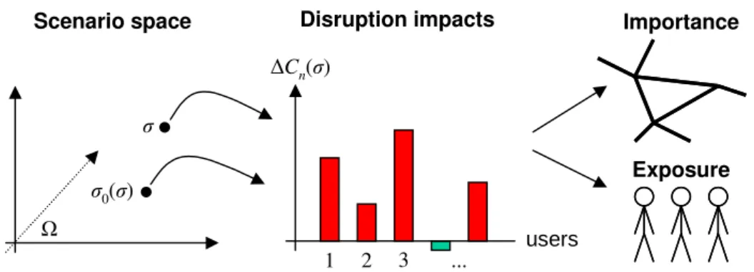
For individualn and disruption scenarioσ we denote this quantity1Cn(σ ). The
framework is illustrated in Figure 3.
Ω σ 0(σ) σ users 1 2 ... ∆C n(σ)
Scenario space Disruption impacts Importance
Exposure
3
Figure 3: An illustration of the framework for vulnerability analysis: With each disruption scenarioσ and corresponding null scenarioσ0(σ )is associated an impact for each user
n, evaluated as the user’s monetary compensating variation for the difference in utility between the two scenarios, 1Cn(σ ). The impacts are aggregated to yield measures of element importance and user exposure.
in an individual’s obtained utility compared to the null scenario for a number of reasons. A component that affects people’s accessibility to critical societal ser-vices and is known to be vital for choices related to travel and activity participation istravel time, and network disruptions often lead to increased travel times for trav-ellers that would normally use the disrupted element or nearby roads indirectly affected by congestion. Beside the possible discomfort of spending an unusually long time travelling, an increase in travel time means that the user will reach (or be reached by) societal services later, or must sacrifice time from other activities
that may be more desirable than travel. With appropriateinformationthe user may
counteract this utility loss to some extent by cancelling the trip, travelling to other destinations or in other ways adjusting her plans. Paper VI proposes an activity-based model to capture some of these utility losses, for work trips in particular, under various levels of available information and schedule flexibility; see further Section 10.
6.1. User exposure
Within this formal framework the exposure of usernto scenarioσ is simply
E(n|σ )=1Cn(σ ). (1)
To formalize theworst-caseexposure of individualn, we partition the
dimen-sions of the scenario space into two subspaces, denoted1 and2, such that
a scenarioσ ∈ can be written asσ = (σ1, σ2), where σ1 ∈ 1andσ2 ∈ 2.
Without loss of generality we assume that we are interested in the worst possible
certain pointσ1. The worst-case exposure ofn with respect to2is then
Ewc(n|σ1, 2)= max
σ2∈2
1Cn(σ1, σ2), (2)
assuming for simplicity that a maximum always exists. As an example, if we
con-sider the worst-case impact of a single link closure in a road network, 2 may
represent the different links in the road network while1may represent different
possible closure durations, times of occurrence etc., of which σ1 is a particular
case.
To formalize theexpectedexposure of individualn, we require that every
con-sidered disruption scenarioσ is associated with a probability of occurrence
nor-malized to 1 across all scenarios. More precisely, we should allow some
dimen-sions of the scenario spaceto be infinite (such as all possible closure durations),
whereas others may be finite (such as all links in the network), which means that probabilities should be represented by a multivariate discrete-continuous
distribu-tion funcdistribu-tionF(x)= P(σ ≤ x)whereσ ≤ x is to be interpreted element-wise.
Given a particular valuex1for the dimensions1one can derive the conditional
distribution functionF2(x2|x1)= P(σ2≤ x2|σ1 =x1). The expected exposure
across all scenarios givenσ1can then be written as
Eexp(n|σ1, 2)= Z
2
1Cn(σ1, σ2)dF2(σ2|σ1). (3)
6.2. Aggregate group exposure
Rather than focusing on single individuals, we may more often be interested in the
exposure of aggregategroupsof individuals. The grouping may be based on some
socioeconomic variables of interest, such as income, gender or residential location. The total exposure of a group g = {n1, . . . ,nNg}, where Ng is the number of
individuals in the group, to scenarioσ is then
TE(g|σ )=X
n∈g
1Cn(σ ). (4)
This represents the total impact of the disruption in economic terms for the group.
Meanwhile, the (mean)user exposureof the group to scenarioσ is simply the total
exposure divided by the number of individuals, i.e.,
UE(g|σ )= 1 Ng
X
n∈g
1Cn(σ ). (5)
Worst-case and expected exposure measures can be defined analogously for a group, in total or per user on average, as for a single user. We include the formal
expressions here for completeness; the worst-case and expected total exposure of the group are
TEwc(g|σ1, 2)= max σ2∈2 TE(g|σ1, σ2), (6) TEexp(g|σ1, 2)= Z 2 TE(g|σ1, σ2)dF2(σ2|σ1), (7)
and the worst-case and expected user exposure are
UEwc(g|σ1, 2)= max σ2∈2 UE(g|σ1, σ2), (8) UEexp(g|σ1, 2)= Z 2 UE(g|σ1, σ2)dF2(σ2|σ1). (9) 6.3. Element importance
As noted above, the road network element involved is only one of many dimensions in which the characteristics of an infrastructure disruption scenario can vary, and our approach to measure the importance of the element is to calculate the total impact of a certain disruption scenario involving the element, conditional on certain
values for the other dimensions. Separating the element, denotede, from the values
for the other dimensions, jointly denoted y, the scenario can be written as σ =
(y,e). The importance of element e can be defined with respect to a particular
group of usersgas
I(e|y,g)=X
n∈g
1Cn(y,e). (10)
By comparing formulas (4) and (10) it may be observed that the importance of
elementeto groupgis identical to the total exposure of groupgto the disruption
scenario involving elemente. In this thesis we will be primarily interested in the
case where the group represents theentire society, i.e., in the overall importance of
elements, in which case the group index will be omitted.
7. From formal to practical measures
In order to conform to the data and models employed in the studies of the road transport system, the practical importance and exposure measures used in Papers I– V are simplified, and superficially quite different, versions of the formal measures above. To begin with the data, the analysis is based on a network representation of the road transport system with nodes representing intersections or dead ends, and
directed links representing road segments between the intersections. Each linkk
has, among other variables, an associated fixed lengthlk and a travel timetk that
To the network special origin/destination (OD) nodes, ordemand nodes, are also connected, representing possible locations where trips enter and leave the road net-work. All OD nodes have associated coordinates that allow them to be partitioned
into geographical regions. Associated with the demand nodes are ODdemand
ma-trices, which contain the number of trips of a certain type (such as work trips) being made during a certain time period (such as the annual average daily travel demand) between each OD node pair under normal conditions.
It should be noted here that the data concerntrips, while our formal measures
concernindividuals. Moving from users to trips could have an influence on the
analysis if a single user makes multiple trips and the impacts of a disruption are not additive across trips (as the model in Paper VI suggests). It could also affect exposure comparisons between groups if the number of trips made per user varies between groups. In this thesis, however, we will not delve further into these issues and will often, somewhat imprecisely, use the term user (as in user exposure) even though the units of analysis will be trips.
Furthermore, the impact models used in Papers I and II–V are adapted to the level of detail in the analysis that the available data allows, which is relatively
coarse. First of all we assume that disruption scenarios consist ofcomplete
clo-suresof one or several links for a certain durationτ, which is typically assumed to be a few days at most. During this time the travel demand is assumed to be inelastic to the disruption, so that all trips between each OD pair that would be made normally will also be made between the same OD pair given the disruption, although possibly postponed until the normal situation is restored. The travel
de-mand per unit time between each OD pair (i, j), denoted xi j, is assumed to be
constant during the disruption and consistent with the OD demand matrix used. Finally, in Papers I–V the compensating variation for each user, or actually trip, related to the disruption is assumed to be proportional to the increase in travel
time or duration of postponement of the trip, collectively called thedelay of the
trip. People thus choose routes and departure times in order to minimize the travel time. Moreover, the proportionality constant, i.e., the value of time, is assumed to be the same for all trips and individuals, so that a delay of a certain length is considered equally bad regardless of who is affected. The value of time, being just a common proportionality constant for all trips, can thus be omitted in relative analyses. Interpreted differently, we ignore the fact that different users on different trips may find the disruption more or less costly and focus on the underlying, more tangible delays. This is problemized in Paper VI and Section 10 below, where we derive functional forms for the relationship between journey delays and costs.
These assumptions mean that a disruption scenario can essentially be described
with only two parameters: The element (the link or group of links) being closed,e,
and (in Papers II–V) the closure duration,τ. Another consequence is that a trip is
also characterized by two factors: the OD pair(i, j)between which the trip takes
disruption.
The total delay compared to the baseline situation (the null scenario with all
links fully operational) for all trips betweeni and j during the disruption given
scenarioσ = (τ,e)is denoted 1Ti je(τ ). The overall importance of elemente is
thus obtained by summing1Ti je(τ )across all OD pairs (compare with (10)),
I(e|τ )=X
i
X
j
1Ti je(τ ). (11)
In Papers I–III and V we study spatial disparities and often partition the trips based on the regions where they start, specifically municipalities or counties. Let
i∈r mean that OD nodeiis located within regionr. The total exposure of region
r to scenario(τ,e)is then (compare with (4))
TE(r|τ,e)=X
i∈r
X
j
1Ti je(τ ). (12)
The total travel demand betweeni and j during the duration of the disruption is
xi jτ, and the user exposure of the region to scenario(τ,e)is (compare with (5))
UE(r|τ,e)= P i∈r P j1T e i j(τ ) P i∈r P j xi jτ . (13)
Theworst-casetotal and user exposure for a given closure durationτ are found
by taking the maximum ofTE(r|τ,e)andUE(r|τ,e)across the set of all
consid-ered elementsE, which corresponds to the general set2in the formal framework.
Similarly, theexpected total and user exposure are found by associating each
el-ement with a normalized closure probability pe(τ ) and calculating the expected
impact across all considered elements as a weighted sum, corresponding to the general integrals in the formal framework. Thus, the worst-case and expected user
exposure of regionr are
UEwc(r|τ,E)=max e∈E UE(r|e, τ ) (14) and UEexp(r|τ,E)=X e∈E pe(τ )UE(r|e, τ ), (15)
with analogous expressions for the worst-case and expected total exposure (com-pare with (6)–(9)).
8. Importance and exposure measures in the thesis
Throughout Papers I–V a large number of variations on the two main themes im-portance and exposure are presented. In actuality the number of different measures introduced is smaller than the numbers of formulas and names would suggest. This is in part an effect of the natural work process, which means that later work has sought to expand and improve upon earlier work. In part it is an effect of the need to appropriately label measures before putting them in relation to each other, which means that the same measure may have different labels in different papers depend-ing on the points of departure. Here we will summarize the various introduced measures and labels and relate them to each other.
8.1. Importance measures
Paper I, the earliest paper, proposes three importance measures: (i) “global”, (ii) “demand-weighted” and (iii) “unsatisfied demand-related” importance. The two
first measures are expressed in terms of changes ingeneralized travel cost rather
than travel time, which essentially corresponds to the compensating variation of the formal framework here; in the practical calculations in the paper, travel time is used for generalized travel cost. The “global” importance measure uses OD pairs rather than trips as the smallest units of analysis. Thus, it focuses more on the potential to travel from anywhere to anywhere and less on the actual travel patterns. This measure is not used in any of the other papers.
The “demand-weighted” importance measure corresponds essentially to the practical importance measure (11) above. A small difference is that the measure in Paper I expresses the average impact per trip rather than the total impact for all trips; this does not affect relative comparisons between links in the same network. A larger difference is that trips that cannot be completed during a link closure (i.e., unsatisfied demand) are not included in the measure, and links of which closures
cause unsatisfied demand, calledcut linksin the thesis, are handled separately with
the “unsatisfied demand-related” measure. In Papers II–V this division into two importance measures is eliminated by introducing an explicit closure duration, as-suming that unsatisfied trips are postponed until after the closure and expressing all impacts in terms of delays.
Paper IIintroduces the concept of (mean) “regional” importance. This is simply the mean importance of the links, more precisely of every road segment of unit length, located within a certain geographical region. With the used model the im-pact of a link disruption is the same regardless of where along the link it occurs. Therefore the unweighted mean importance across every unit length road segment
Paper IIIcontains three named importance measures: (i) “efficiency”, (ii) “equity” and (iii) “equity-weighted” importance. The first measure is identical to the basic importance measure (11) here. The “efficiency” label is added in Paper III because the measure only considers the overall impact of a disruption regardless of how it is distributed among users. The “equity” importance measure, meanwhile, captures only the skewness of the distribution of impacts among users. This measure is not intended as a practical importance measure on its own but is combined with the “efficiency” importance measure to form the third, “equity-weighted” importance measure. With this measure links are considered more important if a given overall impact is more unevenly distributed among users, or put differently, if the disparity in user exposure to the closure of the link is greater.
Paper IVis focused on links’ roles as rerouting alternatives when other links are closed and contains four named link importance measures: (i) “flow-based ef-ficiency”, (ii) “impact-based efef-ficiency”, (iii) “flow-based redundancy” and (iv) “impact-based redundancy” importance. The “flow-based efficiency” importance measure is simply the normal flow across the link. It is considered a measure of importance in this paper because it captures how many users rely on the link for their travel. The “impact-based efficiency” importance measure, just like the “efficiency” importance measure of Paper III, is identical to the basic importance measure (11) here; the prefix “impact-based” is added to distinguish it from the flow-based measure.
A link’s importance as rerouting alternative for other links is called “redun-dancy” importance in Paper IV and represents a quite different form of importance from the other measures in the thesis. “Flow-based redundancy” importance paral-lels “flow-based efficiency” importance by considering the flow that is rerouted to the link when other links are closed, whereas “impact-based redundancy” impor-tance parallels “impact-based efficiency” imporimpor-tance and considers the impact that is avoided by the availability of the link as rerouting alternative.
Paper V, finally, presents a study of “cell” importance, where a cell is an area of a specific shape, size and location that is part of larger grid of cells covering the study area. In the analysis a cell is equivalent to the element consisting of all links intersecting the cell area (fully or partially). Thus, “cell” importance is a special case of the basic element importance measure (11) in Section 7.
8.2. Exposure measures
Paper Istudies in total six different measures of regional exposure to single link closures. That is, users are partitioned into groups based on the geographical re-gions (more specifically, municipalities) in which their trips originate. All six mea-sures, of which three represent worst-case exposure and three represent expected,
here called “average-case”, exposure, actually capture the meanuserexposure of
the region, rather than thetotal exposure. The three variations of each measure
arise in the same way as the three different measures of link importance proposed in the paper: The “global” exposure measure uses OD pairs as the units of analy-sis, the “demand-weighted” exposure measure is based on actual travel demand just like the basic user exposure measure (13) here, whereas the “unsatisfied demand-related” exposure measure handles closures of cut links, i.e., links without alterna-tives. Just as for the importance measures, the need for the “unsatisfied demand-related” exposure measure is avoided in Papers II–V, and the “global” exposure measure is only used in Paper I. It may further be noted that the three measures of expexted or average-case exposure assume an equal probability of closure for all links; this is generalized in subsequent papers.
Paper IIexpands upon the exposure analysis for single link closures in Paper I and introduces the concepts of expected “total” exposure and expected “user” exposure of regions. Just as in (12) and (13) here, “total” exposure refers to the total impact of a certain scenario for all users based in a region, while (mean) “user” exposure refers to the average impact per user based in the region. For the practical calcu-lations of the expected total and user exposure of municipalities and counties it is
assumed in the paper that the closure probability pk of each link is proportional to
the length of the linklk.
Paper Vconsiders regional user exposure to area-covering disruptions. The kind of elements considered is thus not single links but “cells”, i.e., groups of links that all intersect a certain geographical area. The study area is covered with grids of equally sized and shaped cells, and the paper analyses the worst-case user exposure of regions—specifically, counties—across all cells in the grids.
9. Vulnerability and its determinants: Some general results
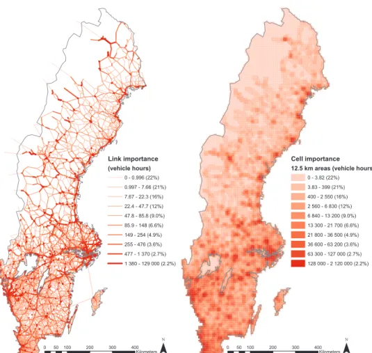
Each of Papers I–V contains a case study in which the considered vulnerability issues and measures are investigated within a model representation of a real road network, in all instances different parts of the Swedish road network. The case studies provide many specific results that are useful for Swedish transport author-ities and other stakeholders, such as the identification of particularly important road segments and particularly exposed regions. However, an important aim of the studies has also been to draw more general conclusions regarding why certain links and areas are more important than others and why certain regions are more exposed than others to various types of scenarios.
Here we summarize some of those findings, which come mainly from the stud-ies presented in Papers II and V. We consider both single link closures and