FlipCut Supertrees: Towards Matrix Representation Accuracy in Polynomial Time

Representation Accuracy in Polynomial Time

Lehrstuhl f¨ur Bioinformatik, Friedrich-Schiller-Universit¨at Jena, Ernst-Abbe-Platz 2, 07743 Jena, Germany,[email protected]

Abstract. In computational phylogenetics, supertree methods provide a way to reconstruct larger clades of the Tree of Life. The supertree problem can be formalized in different ways, to cope with contradictory information in the input. In particular, there exist methods based on encoding the input trees in a matrix, and methods based on finding minimum cuts in some graph. Matrix representation methods compute supertrees of superior quality, but the underlying optimization problems are computationally hard. In contrast, graph-based methods have polynomial running time, but supertrees are inferior in quality. In this paper, we present a novel approach for the computation of supertrees called FlipCut supertree. Our method combines the computation of minimum cuts from graph-based methods with a matrix representation method, namely Minimum Flip Supertrees. Here, the input trees are encoded in a 0/1/?-matrix. We present a heuristic to search for a minimum set of 0/1-flips such that the resulting matrix admits a directed perfect phylogeny. We then extend our approach by using edge weights to weight the columns of the 0/1/?-matrix.

In our evaluation, we show that our method is extremely swift in practice, and orders of magnitude faster than the runner up. Concerning supertree quality, our method is sometimes on par with the “gold standard” Matrix Representation with Parsimony.

This is a preprint of: Malte Brinkmeyer, Thasso Griebel and Sebastian B¨ocker. FlipCut Supertrees: Towards Matrix Representation Accuracy in Polynomial Time. In Proc. of Computing and Combinatorics Conference (COCOON 2011), volume 6842

of Lect Notes Comput Sci, pages 37-48. Springer, Berlin, 2011.

1

Introduction

When studying the relationship and ancestry of current organisms, discovered relations are usually represented as phylogenetic trees: These are rooted trees where each leaf corresponds to a group of organisms, calledtaxon. Inner vertices represent hypothetical last common ancestors of the organisms located at the leaves of its subtree. Supertree methods assemble phylogenetic trees with non-identical but overlapping taxon sets, into a larger supertree that contains all taxa of every input tree and describes the evolutionary relationship of these taxa. Constructing a supertree is easy if no contradictory information is encoded

in the input trees [1]. The major problem of supertree methods is dealing with incompatible data in a reasonable way. It is understood that incompatible input trees are the rule rather than the exception in application.

Current supertree methods can roughly be subdivided into two major families: matrix representation (MR) methods, and graph-based methods with polynomial running time. The former encode inner vertices of all input trees as partial binary characters in a matrix, which is then analyzed using an optimization or agreement criterion to yield the supertree. In 1992, Baum [2] and Ragan [14] independently proposed the matrix representation with parsimony (MRP) method as the first matrix representation method. MRP is by far the most widely used supertree method today, and constructed supertrees are of comparatively high quality. Other variants have been proposed using different optimization criteria, such as matrix representation with flipping (MRF) [5] and matrix representation with compatibility. All MR methods have in common that the underlying optimization problems are NP-hard [5, 7]. So, heuristic search strategies have to be used. Still, running times of MR methods can be prohibitive for large datasets. Recently, Ranwezet al.[16] presented SuperTriplets, a local search heuristic based on triplet dissimilarity and triplet matrix encoding.

A particular matrix representation supertree method is “matrix representa-tion with flipping”: Here, the rooted input trees are encoded in a matrix with entries ‘0’, ‘1’, and ‘?’ [5]. Utilizing the parsimony principle, MRF seeks the minimum number of “flips” 0 → 1 or 1 → 0 in the input matrix that make the resulting matrix consistent with a phylogenetic tree, where ‘?’-entries can be resolved arbitrarily. Evaluations indicate that MRF is on par with the “gold standard” MRP [4].

Graph-based methods make use of a graph to encode the topological information given by the input trees. This graph is used as a guiding structure to build the supertree top-down from the root to the leaves. The first graph-based supertree method was the_Buildalgorithm [1]. This algorithm is only applicable to non-conflicting input trees, and, thus only of limited use in practice. This led to the development of the_MinCut(MC) supertree algorithm [18] and a modified version, _{Modified MinCut}(MMC) supertrees [12]. MC and MMC construct a supertree even if the input trees are conflicting. All three methods share the advantage of polynomial running time, what results in swift computations in applications. On the downside, supertrees constructed by both MC and MMC are consistently of inferior quality compared to those constructed using MR methods [3].

Another graph-based method is PhySIC [15], a so-called veto supertree method. A drawback of veto methods is that they tend to produce unresolved supertrees in case of highly conflicting and/or poorly overlapping input trees. PhySIC IST [17] tries to overcome this drawback by computing non-plenary supertrees: The supertree does not necessarily contain all taxa from the input trees. The Build With Distances algorithm (BWD) [21] is the first graph-based method that uses branch length information from the input trees to build the supertree. It also generalizes the Buildalgorithm but uses branch lengths

to find better vertex partitions in the_Buildgraph. Simulations indicate BWD supertrees are of much better quality than MC and MMC supertrees, but results are not on par with MRP [3].

In this paper, we concentrate on the matrix representation with flipping framework. Recall that the problem is NP-hard [5], and only little algorithmic progress has been made towards its solution. We can test whether an MRF supertree instance admits a perfect phylogeny without flipping in time

O(mnlog2(m+n)) [13]. There exist no parameterized algorithms or non-trivial approximation algorithms in the literature. Chenet al.[4] present a heuristic for MRF supertrees based on branch swapping, and Chimaniet al.[6] introduce an Integer Linear Program to find exact solutions.

Our contributions. Here, we present a novel algorithm, named FlipCut, based on minimizing the number of 0/1-flips in the matrix representation. Our algorithm constructs the phylogenetic tree top-down, minimizing in each step the number of required flips. Running time of our algorithm is comparable to that of the MinCut algorithm: Forn taxa andm internal nodes in the input trees, running time is O(mn3_{). We show that our method usually outperforms}

all other polynomial supertree methods with regards to supertree quality. In contrast to _MinCutsupertrees, our results are interpretable in the sense that we try to minimize a global objective function, namely the number of flips in the input matrix.

2

Preliminaries

Let n be the number of taxa in our study; for brevity, we assume that our set of taxa equals {1, . . . , n}. In this paper, we assume all trees to be rooted phylogenetic trees, that is, there exist no vertices with out-degree one. If there are unrooted trees in the input set, each such tree has to be rooted using an outgroup. In this case, branch lengths (see Sec. 4) of edges incident to the root can be ignored. We are given a set of input treesT1, . . . , Tlwith leaf setL(Ti)⊆

{1, . . . , n}. We assume S

iL(Ti) = {1, . . . , n}. We search for a supertree T of

these input trees, that is, a tree with leave setL(T) ={1, . . . , n}. ForY ⊆ L(T) we define theinduced subtree T|Y ofT where all internal vertices with degree two

are contracted. Some treeT refinesT0ifT0can be reached fromT by contracting internal edges. We say that a supertreeT ofT1, . . . , Tl is aparent treeifT|L(Ti)

refinesT, for alli= 1, . . . , l. In this case,T1, . . . , Tl are calledcompatible.

To cope with incompatibilities in the input, we employ the framework of Flip Supertrees: We encode the input trees in a matrix M with elements in {0,1,?}, where rows correspond to taxa. Each inner vertex (except the root) in each input tree is encoded in one column of the matrix: Entry ‘1’ indicates that the corresponding taxon is a leaf of the subtree rooted in the inner node, whereas all other taxa are encoded ‘0’. The state of taxa that are not part of the input tree is unknown, and represented by a question mark (‘?’). Columns of the matrix are called characters, and we assume that the set of characters equals {1, . . . , m}. Clearly, m ≤ l(n−2). In detail, m is the total number of

non-root inner vertices inT1, . . . , Tl. From the construction ofM, we infer that

each column in M contains a least one ‘0’-entry and at least two ‘1’-entries. The classical (directed)perfect phylogeny model assumes that the matrixM

is binary, and that there exists an ancestral species that possesses none of the characters, corresponding to a row of zeros. This is sometimes referred to as directed perfect phylogeny. Further it is assumed that each transition from ‘0’ to ‘1’ happens at most once in the tree: An invented character never disappears and is never invented twice. According to the perfect phylogeny model, M admits a perfect phylogeny if there is a rooted tree with n leaves corresponding to the

n taxa, where for each character u, there is an inner node w of the tree such that M[t, u] = 1 holds if and only if taxon t is a leaf of the subtree below w, for all t. Given an arbitrary binary matrix M, we may ask whetherM admits a perfect phylogeny. Gusfield [10] shows how to check if a matrix M admits a perfect phylogeny and, if possible, constructs the corresponding phylogenetic tree in timeΘ(mn). There exist several characterizations for matrices that admit a perfect phylogeny, see for example [13].

We now ask whether a matrix with ‘?’-entries allows for a perfect phylogeny, where ‘?’-entries can be arbitrarily resolved to ‘0’ or ‘1’. Interestingly, this can also be decided in ˜O(mn) time [13]. (As usual, the ˜O(·) notation suppresses all poly-log factors.) To resolve incompatibilities among the input trees, the Flip Supertrees model assumes that the matrix M is perturbed. We search for a perfect phylogeny matrixM∗ such that the number of entries where one matrix

M, M∗ contains a ‘0’ and the other matrix a ‘1’, is minimal. This is the number of “flips” required to correct the input matrixM, also referred to as thecost of the instance. Unfortunately, finding the matrix with minimum flip costs is an NP-complete problem, even for an input matrix without ‘?’-entries [5].

To evaluate the quality of our supertrees, we use different measures: Each internal node of a rooted tree T induces a cluster Y ⊆ L(T). The Robinson-Foulds(RF) symmetric distance between two treesT, T0is the number of clusters induced by one tree but not the other, divided by the number of clusters induced by both trees. Another score between trees T, T0 is the maximum agreement subtree (MAST). This is a subset of leaves Y ⊆ L(T) = L(T0) of maximum cardinality such thatT|Y =T0|Y holds. The MAST distance ofT, T0then equals

1− |Y|/|L(T)|.

3

The FlipCut algorithm

The _MinCutalgorithm [18] as well as the _{Modified MinCut} algorithm [12]

construct supertrees by resolving conflicts in the input trees in a recursive top-down procedure. This has been adapted from the _Build algorithm [1] that returns a supertree only if the input trees are compatible. A related algorithm was given by Pe’eret al.[13]. This algorithm tests whether an MFST instance

M allows for a perfect phylogeny without flipping, by resolving all ‘?’-entries. In fact, these two problems are equivalent: The input trees can be encoded in a matrix M as described in Sec. 2. Also, an input matrix M with m columns

can be transformed intominput trees, where each columncis transformed into a tree with those taxa t satisfyingM[t, c]6=?, having a single non-trivial clade with taxa t such that M[t, c] = 1. In the following, we show how to apply the idea of finding minimum cuts to the algorithm of Pe’eret al..

For a subset S ⊆ {1, . . . , n} of taxa and a subset D ⊆ {1, . . . , m} of characters, theFlipCut graphG(S, D) is a bipartite graph with vertex setsSand

D, and an edge (t, c) is present in G(S, D) if and only ifM[t, c] = 1, fort ∈S

andc∈D. A character vertexc∈Dissemiuniversal (inS, D) ifM[t, c]∈ {1,?} holds for all t∈S. We immediately remove all semiuniversal character vertices fromG(S, D), as all ‘?’-entries can be resolved to ‘1’ without flipping [13].

The algorithm of Pe’er et al. proceeds as follows: We start with S ←

{1, . . . , n} andD← {1, . . . , m}. We then construct the FlipCut graphG(S, D).

If this graph is connected, the algorithm terminates, as there is no perfect phylogeny resolving M. Otherwise, we recursively repeat for each connected componentS0_{, D}0_{of the FlipCut graph with|S}0_{|>1. In case the algorithm does} not terminate early, then the setsS0 of taxa computed during the course of the algorithm, define the rooted phylogenetic tree.

Assume thatG(S, D) is connected at some point of the algorithm — how can we disconnect the graph by means of modifying the input matrixM? Obviously, it does not help to insert new edges in G(S, D). Removing an edge (t, c) from

G(S, D) can be achieved by two different operations: either flip M[t, c] from ‘1’ to ‘0’, or make character c semiuniversal by flipping all entries satisfying

M[t0, c] = 0 to ‘1’, for t0 ∈ S. Recall that any semiuniversal character c is deleted immediately, resulting in the deletion of all edges incident to c. This comes at the cost of w(c) := #{t ∈ S : M[t, c] = 0} flips in the matrix. To disconnect G(S, D) we can use an arbitrary combination of these edge deletion operations.

Formally, we assume all edges inG(S, D) to have unit weight, and that each character vertexchas weightw(c). The weight of a bipartition of taxa vertices is the minimal cost of a set of edge and vertex deletions, such that the two subsets of taxa vertices lie in separate components of the resulting graph. We search for a bipartition of minimal weight.

Clearly, this problem is closely related to finding minimal cuts in an undirected graph. Unfortunately, there exist two important differences here: First, we are not searching for an arbitrary cut in the graphG(S, D) but instead, require that the set of taxa vertices is partitioned. Second, these algorithms do not allow us to delete vertices. We conjecture that the first modification is relatively easy to overcome. However, it is not obvious how to include vertex deletions in these algorithms.

To this end, we drop back to an older approach for finding minimum cuts: We fix one taxon vertex s, and for all other taxa vertices t we search for a minimum s-t-cut, allowing vertex deletions. Among these cuts, the cut with minimal weight is the solution to the above problem. To find a minimum s-t -cut with vertex deletions, we transformG(S, D) into a directed networkH(S, D) with capacities: Each taxa vertextis also a vertex in the network, each character

vertex c is transformed to two vertices c− and c+ plus an arc (c−, c+) in the

network, and an edge (t, c) in G(S, D) is transformed to two arcs (t, c−) and (c+, t) in the network. Arcs (c−, c+) have weightw(c), all other arcs have unit

weight. By the generalized min-cut max-flow theorem, finding a minimum cut in

G(S, D) is equivalent to computing a maximum flow in the networkH(S, D) [8]. Note that for all taxas, t, the maximums-t-flow inH(S, D) equals the maximum

t-s-flow. We reach:

Lemma 1. Let S ⊆ {1, . . . , n}, D ⊆ {1, . . . , m}, and M ∈ {0,1,?}m×n_{. We}

construct the network H := H(S, D) for the input matrix M. The minimum number of 0/1 flips required inM to make the induced FlipCutgraphG(S, D) disconnected, equals the minimum cost of a minimum1-t-cut in the networkH, over all t= 2, . . . , n.

We now proceed in a recursive top-down procedure to construct the supertree, similar to [12, 13, 18]. Due to space constraints, we omit the simple pseudocode of the algorithm. The subsetsS ⊆ {1, . . . , n}that are output during the course of the algorithm, form a hierarchy which can be transformed into the desired supertree. As the algorithm reproduces that of Pe’eret al.in case the input trees are compatible or, equivalently, in case the input matrix allows for a perfect phylogeny without flipping, we infer:

Lemma 2. In case the input matrix M allows for a perfect phylogeny without

flipping, then the _FlipCutalgorithm returns the perfect phylogeny tree. What is the running time of the above algorithm? At mostn−1 minimum cuts have to be computed in total, as this is the number of inner nodes in the resulting phylogenetic tree. We reach a running time ofO(n·T(m, n)) whereT(m, n) is the time required for computing all maximum 1-t-flows in the networksH(S, D) with at mostmcharacter vertices andntaxa vertices. The running time is dominated by the algorithm we use for constructing maximum flows. For a network H = (V, E), Hao and Orlin [11] compute maximum flows from one source to all other vertices inO |V| · |E| ·log(|V|2/|E|)

time, using the maximum flow algorithm of Goldberg and Tarjan. For a bipartite graph with vertex set V1 ∪V2 and

|V1| ≤ |V2|, running time can be improved toO |V1| · |E| ·log(|V1| 2

/|E|)

[11]. Our networks H(S, D) are bipartite and have O(n+m) vertices and O(mn) edges, and we may assume n≤m. So, a minimum cut with vertex deletions in

G(S, D) can be computed inO(mn2_{) time. We infer:}

Lemma 3. Given an input matrixM over{0,1,?}forntaxa andmcharacters,

the _FlipCutalgorithm computes a supertree in O(mn3_)time.

As presented here, the_FlipCutalgorithm may compute different solutions for the same input: This is because there can be several co-optimal minimum cuts, and our algorithm arbitrarily chooses one of these cuts. We can solve this by removing all edges and vertices that are part ofat least oneminimum cut, similar to theMinCutalgorithm [18]. In the following, we ignore this modification: We weight all edges with real numbers, so the existence of several minimum cuts of identical weight is practically impossible.

4

Using branch lengths

To compare branch lengths from different trees in a real-world study, we first have to normalize them. Due to space constraints, we defer the details to the full version of this paper. We can use branch lengths in a straightforward fashion: We weight each column of the matrix by the length of the branch that was responsible for generating the column. This can be easily incorporated into the

FlipCutgraph, by weighting edges and character vertices. In this way, flipping

an entry is cheaper for those branches that are possibly wrong, and harder for those branches that are most likely true.

In our evaluations, a different weighting called “Edge & Level” showed a better performance: Each character vertex c corresponds to an internal edge

e = (u, v) in one of the input trees, inducing the corresponding column in the matrixM. We set the weight of charactercand, hence, the corresponding column inM tol(c) :=w(e)·depth(v). Here,l(c) is the length of branche, anddepth(v) is thenumber of edges on the path from the root tov in the input tree.

5

The undisputed sibling problem

Given a set of input trees, assume that some taxon x appears as a sibling of another taxon y in all the input trees in which it is present at all. In other words, for all trees where x is present, we also find y, and both are siblings. We call such x an undisputed sibling. Then, it is reasonable to assume thatx

is also a sibling of y in the supertree, possibly accompanied by other siblings. Unfortunately, Flip Supertrees does not necessarily enforce this: Minimizing the number of flips, it is sometimes cheaper to separatexandy. This is a seemingly rare but still undesirable effect of this objective function.

To counter the above effect, we use a data reduction rule that is applied to all input trees before we computeFlipCutsupertrees: If there is an undisputed siblingxofy, then removexfrom all input trees. We repeat this until we find no more undisputed siblings. Note that by removing an undisputed sibling, we might produce new undisputed siblings. After we have computed the supertree, we re-insert all undisputed siblings in reverse order. Ifyhas more than one undisputed sibling at the same time, we re-insert all siblings in one node, resulting in a polytomy in the supertree.

There exist two possibilities to remove the undisputed sibling x: Either we simply deletex from the input trees, resulting in a deletion of rowxfrom the input matrix, and subsequent deletion of all columns that have only a single ‘1’-entry. Or, we decide to add the weight of xandy in those trees where xis removed. In the matrix, we then treat 0/1-entries to be weighted by a positive integer. In our implementation, we concentrate on the first variant.

6

Experiments

We want to evaluate the performance of the FlipCut supertree method in comparison to Matrix Representation with Parsimony (MRP), Matrix

Repre-sentation with Flipping (MRF), Build With Distances (BWD), PhySIC IST, and SuperTriplets. Recall that MC and MMC supertrees are of comparatively low quality, and consistently worse than BWD [3], so we excluded these two methods from our study. We use simulated data in our evaluation since here, the true tree (or model tree) is known. Thus, results of different methods can be compared at an absolute scale. Our evaluation study proceeds in the usual fashion: A model tree is generated, and gene sequences are evolved along the branches. Sequences at the taxa of the model tree are used as datasets from which source trees for a supertree method are inferred. Finally, the resulting supertree is compared to the model tree using distance or similarity measures.

For our simulations, we used a dataset1 _{that was generated using the}

SMIDgen protocol described in [20]. Compared to previous protocols, this protocol better reflects data collection processes used by systematists when gathering empirical data. This includes creation of densely-sampled clade-based trees as well as sparsely-sampled scaffold trees. Model trees having either 100, 500 or 1000 taxa were generated with 30 replicates for the 100 and 500 taxon case, and ten replicates for the 1000 taxa case. We defer further details to the full version of this paper.

For the simulation study, we know that all branch lengths are computed under the same model of sequence evolution. This can be seen as an optimal condition for the BWD andFlipCutalgorithm. Again, we defer the evaluation on whether branch length normalization changes the quality of reconstructed supertrees, to the full version of this paper.

We implemented the FlipCut algorithm in Java as part of the EPoS

framework [9]. In order to to illustrate the influence of branch-length to our approach, we use two different weighting schemes for edges and character vertices in the graph model: First, unit costs, where branch lengths are ignored. Here, the cost of deleting an edge is one, and the cost of deleting a character vertexc

is just the number of zeros in the corresponding column in matrixM. Second, “Edge & Level”, where we make use of branch lengths. We multiply deletion costs for character vertexcand all edges incident tocbyw(c) =l(e)·depth(v). Here, l(e) is the length of branche= (u, v),depth(v) is the number of edges on the path from the root tov, andc corresponds tov.

MRP supertrees were computed using PAUP* 4.0b10 [19] with TBR branch swapping strategy, random addition of sequences, no limit on the maximal number of trees in memory, and 100 replicates. MRF supertrees were generated using the implementation provided by Duhong Chen2_{, also with the TBR branch}

swapping strategy. For 100 taxa model trees, we used 30 replicates for the search, and in case of 500 and 1000 taxa model trees only ten replicates, because on our cluster the implementation failed with more replicates. BWD supertrees were constructed using the implementation by Stephen J. Willson.3 For the PhySIC IST supertrees [17] we used the implementation provided by

1

http://www.cs.utexas.edu/~phylo/datasets/supertrees.html

2 _{http://genome.cs.iastate.edu/CBL/download/} 3

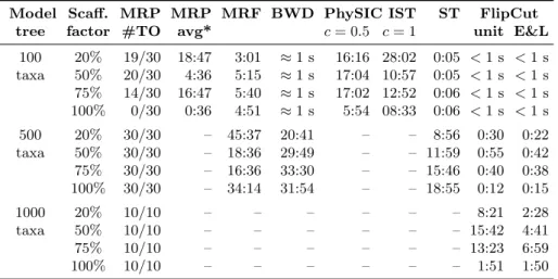
Model Scaff. MRP MRP MRF BWD PhySIC IST ST FlipCut

tree factor #TO avg* c= 0.5 c= 1 unit E&L

100 20% 19/30 18:47 3:01 ≈1 s 16:16 28:02 0:05 <1 s <1 s taxa 50% 20/30 4:36 5:15 ≈1 s 17:04 10:57 0:05 <1 s <1 s 75% 14/30 16:47 5:40 ≈1 s 17:02 12:52 0:06 <1 s <1 s 100% 0/30 0:36 4:51 ≈1 s 5:54 08:33 0:06 <1 s <1 s 500 20% 30/30 – 45:37 20:41 – – 8:56 0:30 0:22 taxa 50% 30/30 – 18:36 29:49 – – 11:59 0:55 0:42 75% 30/30 – 16:36 33:30 – – 15:46 0:40 0:38 100% 30/30 – 34:14 31:54 – – 18:55 0:12 0:15 1000 20% 10/10 – – – – – – 8:21 2:28 taxa 50% 10/10 – – – – – – 15:42 4:41 75% 10/10 – – – – – – 13:23 6:59 100% 10/10 – – – – – – 1:51 1:50

Table 1.Running times (min:sec) of the different algorithms.MRP #TOis the number of timeouts of MRP where computation was stopped after one hour, andMRP avg* is the average running time of those runs that stopped before the time limit.ST is the SuperTriplets method. BWD computed four supertrees for different distance models within the measured time.

the authors.4 PhySIC IST offers a parameter to tune the method from “veto” to “voting-like”. In our simulation, we used 0.5 and 1 as parameter settings. We generated SuperTriplets supertrees [16] using the implementation provided by the authors.5_{. All computations were performed on a Linux cluster of AMD}

Opteron-2378, 2.4 GHz CPUs, with 16 GB of memory.

7

Results

We first consider running times of MRP, MRF, BWD, PhySIC IST, Super-Triplets, and the _FlipCut algorithm presented here, see Table 1. For each instance, we use a running time limit of one hour in case of 100 and 500 taxon model trees, and two hours in case of 1000 taxon model trees. Entries ‘–’ indicate that no instance was finished within the time limit: Regarding MRP, PAUP* returns a consensus of the current trees in memory if the time limit is exceeded. In contrast, the MRF implementation returns no tree. PhySIC IST crashes for model tree sizes of 500 and 1000 taxa, and the SuperTriplets implementation crashes for model tree sizes of 1000 taxa.

PAUP* often runs into timeouts even for the smallest instances containing only 100 taxa. Similarly, PhySIC IST can process only instances of this size. MRF, BWD, and SuperTriplets can process instances with up to 500 taxa in less than one hour. In contrast, our FlipCut method is several orders of

4 _{http://www.atgc-montpellier.fr/physic_ist/with option ‘-c’} 5

magnitude faster than any other method. Even large instances with 1000 taxa can be processed in a matter of minutes.

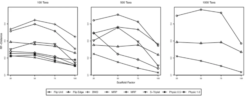
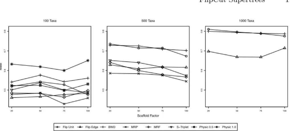
Next, we investigate the accuracy of reconstructed supertrees. Results are shown in Fig. 1 and 2. Recall thatPhySIC IST usually computes non-plenary supertrees: Here, we first restrict the model tree to the taxon set of the supertree. This favors PhySIC IST for all distance measures but the MAST distance, so PhySIC IST results must be interpreted with some caution.

For the RF distance, we see that for all model tree sizes, MRP supertrees are of the best quality. For 100 taxa model trees, MRP, thePhySIC IST variants, and MRF show the best performance, followed by_FlipCut“Edge & Level”. For 500 taxa model trees, performance from best to worst is: MRP, MRF,FlipCut

“Edge & Level”, BWD, and FlipCutunit costs. SuperTriplets performs good for small and large scaffold density. For 100 taxa model trees, performance from best to worst is: MRP,FlipCut“Edge & Level”, andFlipCutunit costs.

The the MAST distance and 100 taxa model trees,PhySIC IST 1 performs significantly worse than all other methods. MRP outperforms the other methods only with input tree sets with a scaffold density of 75% and 100%. Both_FlipCut “Edge & Level” and MRP compute supertrees such that the MAST between supertree and model tree consistently contains more than half of the taxa. MRP, MRF, and_FlipCut“Edge & Level” perform almost on par. For 500 taxa model trees, we see three groups: MRP and MRF perform best, closely followed by

FlipCut “Edge & Level” and SuperTriplets. Performance of FlipCut unit

cost and BWD is much worse. Finally, for 1000 taxa model trees, MRP performs best, butFlipCut“Edge & Level” is on second place with similar performance except for scaffold density 100%.

0.1 0.2 0.3 0.4 100 Taxa RF−Distance 20 50 75 100 0.1 0.2 0.3 0.4 500 Taxa Scaffold Factor 20 50 75 100 0.1 0.2 0.3 0.4 1000 Taxa 20 50 75 100

Flip Unit Flip Edge BWD MRP MRF S−Triplet Physic 0.5 Physic 1.0

Fig. 1.Simulation results, quality of reconstructed supertrees. We plot the Robinson-Foulds distance between the calculated supertree to the true model tree, averaged over all simulation replicates. From left to right, model trees with 100, 500, and 1000 taxa.

0.5 0.6 0.7 0.8 100 Taxa Mast 20 50 75 100 0.5 0.6 0.7 0.8 500 Taxa Scaffold Factor 20 50 75 100 0.5 0.6 0.7 0.8 1000 Taxa 20 50 75 100

Flip Unit Flip Edge BWD MRP MRF S−Triplet Physic 0.5 Physic 1.0

Fig. 2. Simulation results, quality of reconstructed supertrees. We plot the MAST distance between the calculated supertree and the true model tree, averaged over all simulation replicates. From left to right, model trees with 100, 500, and 1000 taxa.

8

Conclusion

We have presented a novel supertree method named _FlipCutsupertrees. Our method combines the intuition behind both Minimum Flip and _MinCut su-pertrees. We have also presented a heuristic that ensures that undisputed siblings will be present in the constructed supertree. The_FlipCutsupertree method has polynomial running time and is extremely swift in practice. Regarding supertree quality, performance of the _FlipCutalgorithm is sometimes even on par with MRP.

Besides the much better performance in simulations, FlipCut supertrees offer a fundamental advantage overMinCutsupertrees: We have defined a global objective function that we want to minimize, whereas no such objective can be defined forMinCutand its derivatives. Besides the theoretical amenity of such a objective function, this also has practical implications: We can compare the quality of different supertrees based on our objective function; and we can also compare the quality of partial solutions. We conjecture that this fact will allow us to further improve the quality of _FlipCut supertrees. Finally, we want to evaluate methods for weighting the edges in the _FlipCutgraph. The “Edge & Level” weighting presented here, is merely meant to demonstrate the impact of weighting edges on the quality of constructed supertrees.

Acknowledgments. Additional implementation by Markus Fleischauer.

References

1. A. V. Aho, Y. Sagiv, T. G. Szymanski, and J. D. Ullman. Inferring a tree from lowest common ancestors with an application to the optimization of relational expressions. SIAM J. Comput., 10(3):405–421, 1981.

2. B. R. Baum. Combining trees as a way of combining data sets for phylogenetic inference, and the desirability of combining gene trees. Taxon, 41(1):3–10, 1992.

3. M. Brinkmeyer, T. Griebel, and S. B¨ocker. Polynomial supertree methods revisited. InProc. of Pattern Recognition in Bioinformatics (PRIB 2010), volume 6282 of Lect. Notes Comput. Sc., pages 183–194. Springer, 2010.

4. D. Chen, O. Eulenstein, D. Fern´andez-Baca, and J. G. Burleigh. Improved heuristics for minimum-flip supertree construction.Evol. Bioinform. Online, 2:391– 400, 2006.

5. D. Chen, O. Eulenstein, D. Fern´andez-Baca, and M. Sanderson. Minimum-flip supertrees: complexity and algorithms. IEEE/ACM Trans. Comput. Biol. Bioinform., 3(2):165–173, 2006.

6. M. Chimani, S. Rahmann, and S. B¨ocker. Exact ILP solutions for phylogenetic minimum flip problems. In Proc. of ACM Conf. on Bioinformatics and Computational Biology (ACM-BCB 2010), pages 147–153, 2010.

7. W. Day, D. Johnson, and D. Sankoff. The computational complexity of inferring rooted phylogenies by parsimony. Math. Biosci., 81:33–42, 1986.

8. L. R. Ford and D. R. Fulkerson. Flows in Networks. Princeton University Press, Princeton, New Jersey, 1962.

9. T. Griebel, M. Brinkmeyer, and S. B¨ocker. EPoS: a modular software framework for phylogenetic analysis. Bioinformatics, 24(20):2399–2400, 2008.

10. D. Gusfield. Efficient algorithms for inferring evolutionary trees.Networks, 21:19– 28, 1991.

11. J. X. Hao and J. B. Orlin. A faster algorithm for finding the minimum cut in a directed graph. J. Algorithms, 17(3):424 – 446, 1994.

12. R. D. M. Page. Modified mincut supertrees. InProc. of Workshop on Algorithms in Bioinformatics (WABI 2002), volume 2452 ofLect. Notes Comput. Sc., pages 537–552. Springer, 2002.

13. I. Pe’er, T. Pupko, R. Shamir, and R. Sharan. Incomplete directed perfect phylogeny. SIAM J. Comput., 33(3):590–607, 2004.

14. M. A. Ragan. Phylogenetic inference based on matrix representation of trees.Mol. Phylogenet. Evol., 1(1):53–58, 1992.

15. V. Ranwez, V. Berry, A. Criscuolo, P.-H. Fabre, S. Guillemot, C. Scornavacca, and E. J. P. Douzery. PhySIC: a veto supertree method with desirable properties.Syst. Biol., 56(5):798–817, 2007.

16. V. Ranwez, A. Criscuolo, and E. J. P. Douzery. Supertriplets: a triplet-based supertree approach to phylogenomics. Bioinformatics, 26(12):i115–i123, 2010. 17. C. Scornavacca, V. Berry, V. Lefort, E. J. P. Douzery, and V. Ranwez. PhySIC IST:

cleaning source trees to infer more informative supertrees. BMC Bioinformatics, 9:413, 2008.

18. C. Semple and M. Steel. A supertree method for rooted trees. Discrete Appl. Math., 105(1-3):147–158, 2000.

19. D. Swafford. Paup*: Phylogenetic analysis using parsimony (*and other methods), 2002. Version 4.

20. M. S. Swenson, F. Barbancon, T. Warnow, and C. R. Linder. A simulation study comparing supertree and combined analysis methods using SMIDGen.Algorithms Mol. Biol., 5(1):8, 2010.

21. S. J. Willson. Constructing rooted supertrees using distances. Bull. Math. Biol., 66(6):1755–1783, 2004.