Boosting for Learning Multiple Classes with Imbalanced Class Distribution
Yanmin Sun
Department of Electrical
and Computer Engineering
University of Waterloo
Waterloo, Ontario, Canada
Mohamed S. Kamel
Department of Electrical
and Computer Engineering
University of Waterloo
Waterloo, Ontario, Canada
Yang Wang
Pattern Discovery
Software Systems Ltd.
554 Parkside Drive
Waterloo, Ontario, Canada
Abstract
Classification of data with imbalanced class distribution has posed a significant drawback of the performance attain-able by most standard classifier learning algorithms, which assume a relatively balanced class distribution and equal misclassification costs. This learning difficulty attracts a lot of research interests. Most efforts concentrate on bi-class problems. However, bi-class is not the only scenario where the class imbalance problem prevails. Reported solutions for bi-class applications are not applicable to multi-class problems. In this paper, we develop a cost-sensitive boost-ing algorithm to improve the classification performance of imbalanced data involving multiple classes. One barrier of applying the cost-sensitive boosting algorithm to the imbal-anced data is that the cost matrix is often unavailable for a problem domain. To solve this problem, we apply Genetic Algorithm to search the optimum cost setup of each class. Empirical tests show that the proposed cost-sensitive boost-ing algorithm improves the classification performances of imbalanced data sets significantly.
1
Introduction
Classification is an important task of knowledge discov-ery in databases (KDD) and data mining. Recently, reports from both academy and industry indicate that the imbal-anced class distribution of a data set has posed a serious dif-ficulty to most classifier learning algorithms which assume a relatively balanced distribution [9, 12]. Imbalanced class distribution is characterized as that there are many more instances of some classes than others. With imbalanced data, classification rules that predict the small classes tend to be fewer and weaker than those that predict the prevalent classes; consequently, test samples belonging to the small classes are misclassified more often than those belonging
to the prevalent classes. Standard classifiers usually per-form poorly on imbalanced data sets because they are de-signed to generalize from training data and output the plest hypothesis that best fits the data. Therefore, the sim-plest hypothesis pays less attention to rare cases. However, in many cases, identifying rare objects is of crucial impor-tance; classification performances on the small classes are the main concerns in determining the property of a classifi-cation model.
The difficulty raised by the class imbalance problem with both academic research and practical applications in the community of machine learning and data mining attracts a lot of research interests. Reported works focus on three aspects of the class imbalance problem: 1) what are the proper evaluation measures of classification performance in the presence of the class imbalance problem? 2) what is the nature of the class imbalance problem, i.e. in what do-mains do class imbalances most hinder the performance of a standard classifier? [9]; and 3) what are the possible so-lutions in dealing with the class imbalance problem? With regard to the first aspect, it is stated that accuracy is tradi-tionally the most commonly used measure in both assessing the classification models and guiding the search algorithms. However, for a classification model induced from a data set with imbalanced class distribution, accuracy is no longer a proper measure since rare classes have very few impact on accuracy than prevalent classes [11]. Some other evaluation measures, such as recall, precision, F-measure, G-mean and Receiver Operation Characteristic (ROC) Curve Analysis, are then explored and proposed as more proper evaluation measures [1, 10, 16]. With respect to the second aspect, a thorough study can be found in [9]. Other relevant works are reported in [10, 23, 24]. These studies show that the imbalanced class distribution is not the only factor that hin-ders the classification performance. Other factors that de-teriorate the performance include the training sample size, the separability and the presences of sub-concepts within a group. The third aspect is the focus of most publications
ad-dressing the class imbalance problem. Almost all reported solutions are designed for the bi-class scenario.
In a bi-class application, the imbalanced problem is ob-served as one class is represented by a large amount of sam-ples while the other is represented by only a few. The class with very few training samples and usually associated with high identification importance, is referred as the positive class; the other one as the negative class. The learning ob-jective of this kind of data is to obtain a satisfactory identi-fication performance on the positive (small) class. Reported solutions for the bi-class applications can be categorized as data level and algorithm level approaches [2]. At the data level, the objective is to re-balance the class distribution by re-sampling the data space including oversampling in-stances of the positive class and undersampling inin-stances of the negative class, sometimes, uses the combination of the two techniques [2]. At the algorithm level, solutions try to adapt the existing classifier learning algorithms to bias to-wards the positive class, such as cost sensitive learning [15] and recognition based learning [8]. In addition to these so-lutions, another approach is boosting. Boosting algorithms change the underlying data distribution and apply the stan-dard classifier learning algorithms to the revised data space iteratively. From this point of view, boosting approaches should be categorized as solutions at data level.
The AdaBoost (Adaptive Boosting) algorithm [5, 19] is reported as an effective boosting algorithm to improve clas-sification accuracies of any “weak” learning algorithms. It weighs each sample reflecting its importance and places the most weights on those examples which are most of-ten misclassified by the preceding classifiers. This forces the following learning to concentrate on those samples hard to be correctly classified. When the AdaBoost algorithm is adapted to tackle the class imbalance problem, advan-tages are: 1) it is applicable to most classifier learning al-gorithms; 2) the sample weighting strategy of the AdaBoost algorithm is equivalent to re-sampling the data space com-bining both up-sampling and down-sampling; 3) as a re-sampling method, AdaBoost updates the data space auto-matically eliminating the extra learning cost for exploring the optimal class distribution; and 4) resampling through weighting samples has little information loss and the Ad-aBoost algorithm is stated to be immune to overfitting [6]. Boosting is therefore an attractive technique in tackling the class imbalance problem. Within the bi-class applications, some variants of the AdaBoost algorithm in tackling the im-balance problem are reported, such as AdaCost [4], CSB1 and CSB2 [21], RareBoost [11] and AdaC1, AdaC2 and AdaC3 [20]. These boosting algorithms inherit the general learning framework of the AdaBoost algorithm and feed misclassification costs into the weight update formula of AdaBoost to distinguish the uneven learning importance be-tween classes. As these algorithms use cost items, they are
also regarded as cost-sensitive boosting algorithms. Yet bi-class is not the only scenario where the class im-balance problem prevails. In practice, most applications have more than two classes where the unbalanced class dis-tributions hinder the classification performance. Solutions for bi-class problems are not applicable directly to multi-class cases. One possible solution is to convert a multi-multi-class problem into a number of bi-class problems, i.e., classify-ing each individual class versus all the other classes. The obvious drawbacks of this treatment are: 1) to learn an identification model for each class is expensive in training; 2) results of each class label assignment are not compara-ble due to the decision can be made differently for differ-ent classes; and 3) one class versus the other classes will worse the imbalanced distribution even more for the small classes. Even though cost-sensitive boosting algorithms can be adopted for multiple class applications, research efforts are still limited to bi-class cases. One reason is that the cost matrix is often unavailable for a given problem do-main. For sensitive learning and/or measures, the cost-matrix is assumed known for different types of errors or samples. Without the cost matrix, experiments for bi-class problems were conducted by set up a range of cost factors manually. Such a strategy is not applicable to multiple class cases since to figure out satisfactory cost values manually for multiple classes is a non-trivial job. Hence, searching a efficient cost setup becomes a critical issue for applying the cost-sensitive boosting approach to multiple class applica-tions. To our knowledge, there is no reported work on the class imbalance problem addressing multiple class cases.
In this paper, we develop a cost-sensitive boosting al-gorithm for the class imbalance problem in the scenario of multiple classes. We extended the original AdaBoost al-gorithm to multi-class cases. The straightforward gener-alization is called AdaBoost.M1 [5]. By using the same inference methods provided in [5, 18], we prove that the upper bound error of the final hypothesis output by Ad-aBoost.M1 holds the same format as that by AdaBoost. Thus, the crucial weight update parameter of AdaBoost.M1 is selected as the same as that of AdaBoost. Among those reported cost-sensitive boosting algorithms, we select and extend AdaC2 [20] to multi-class cases. The extension in-heriting the framework of AdaBoost.M1 is therefore de-noted as AdaC2.M1. We then compare the weighting strat-egy of AdaC2.M1 with that of AdaBoost.M1 to explore the boosting efficiency of AdaC2.M1. To decide the cost se-tups that can be applied to the AdaC2.M1 algorithm, we apply Genetic Algorithm (GA) which achieves outstanding performance in finding optimal parameters. To evaluate the performance , three “real world” data sets are tested since their classification performances are hindered by their im-balanced class distributions.
Given:(x1, y1),· · ·,(xm, ym)wherexi ∈ X,yi ∈ Y =
{−1,+1}
InitializeD1(i) = 1/m. Fort= 1,· · ·, T:
1. Train base learnerht→Y using distributionDt
2. Choose weight updating parameter:αt
3. Update and normalize sample weights: Dt+1(i) = Dt(i)exp(−αtht(xi)yi)
Zt (1)
Where,Ztis a normalization factor.
Output the final classifier: H(x) =sign(
T
X
t=1
αtht(x)) (2)
Figure 1. AdaBoost Algorithm
2
AdaBoost Algorithm
The original AdaBoost algorithm reported in [5, 19] takes as input a training set{(x1, y1),· · ·,(xm, ym)}where
eachxiis an n-tuple of attribute values belonging to a
cer-tain domain or instance spaceX, andyiis a label in a label
setY = {−1,+1}in the context of bi-class applications. The Pseudocode for AdaBoost is given in Figure 1.
It has been shown in [19] that the training error of the final classifier is bounded as
1 m|{i:H(xi)6=yi}| ≤ Y t Zt (3) Let f(x) = T X t=1 αtht(x)
By unraveling the update rule of Equation 1, we have that
Dt+1(i) = exp(− P tαtht(xi)yi) mQtZt = exp(−yif(xi)) mQtZt (4)
By the definition of the final hypothesis of Equation 2, if H(xi) 6= yi, the yif(xi) ≤ 0 implying that
exp(−yif(xi))≥1. Thus,
[H(xi)6=yi]≤exp(−yif(xi)). (5)
where for any predicateπ, [π] =
n
1 ifπholds
0 otherwise (6)
Combining Equation 4 and 5 gives the error upper bound of Equation 3 since 1 m X i [H(xi)6=yi]≤ 1 m X i exp(−yif(xi)) (7) = X i (Y t Zt)Dt+1(i) = Y t Zt (8)
To minimize the error upper-bound, on each boosting round, the learning objective is to minimize
Zt = X i Dt(i)exp(−α tyiht(xi)) (9) = X i Dt(i)(1 +yiht(xi) 2 e −α+1−yiht(xi) 2 e α)(10)
Then, by minimizingZton each round,αtis induced as
αt= 1 2log( X i,yi=ht(xi) Dt(i) X i,yi6=ht(xi) Dt(i)) (11)
The sample weight updating goal of AdaBoost is to de-crease the weight of training samples which are correctly classified and increase the weights of the opposite part. Therefore,αtshould be a positive value demanding that the
training error should be less than randomly guessing (0.5) based on the current data distribution. That is
X i,yi=ht(xi) Dt(i)> X i,yi6=ht(xi) Dt(i) (12)
3
AdaBoost.M1 Algorithm
The original AdaBoost algorithm is designed for bi-class applications. There are several methods of extending Ad-aBoost to the multi-class cases. The straightforward gener-alization one, called AdaBoost.M1 in [5], is adequate when the base learner is effective enough to achieve reasonably high accuracy (training error should be less than 0.5).
AdaBoost.M1 differs slightly from AdaBoost. The main differences are the replacements of the weight update for-mula of Equation 1 by:
Dt+1(i) = Dt(i)exp(−αtI[ht(xi) =yi])
Zt (13)
where,Ztis a normalization factor, and
I[ht(xi) =yi] =
n
+1 ifht(xi) =yi
−1 ifht(xi)6=yi (14)
H(x) =argmax Ci ( T X t=1 αt[ht(x) =Ci]) (15)
By using the same inference methods provided in [5, 18], we can prove the following bound still holds on the training error of the final hypothesis outputH(x)(Equation 15) by AdaBoost.M1: 1 m|{i:H(xi)6=yi}| ≤ Y t Zt (16) where Zt= X i Dt(i)exp(−αtI[ht(xi) =yi]) (17)
To prove this theorem, we reduce the setup for Ad-aBoost.M1 to an instantiation of AdaBoost. For clarity, variables in the reduced AdaBoost space are marked with tildes. For each of the given samples(xi, yi), an AdaBoost
sample(˜xi,y˜i)is generated, wherex˜i =xiandy˜i= 1, i.e.,
each AdaBoost sample has label 1. The AdaBoost distribu-tionD˜ over samples is set to be equal to the AdaBoost.M1 distributionD. On each round, an AdaBoost hypothesis˜ht
is defined as ˜ ht(xi) =I[ht(xi) =yi] = n +1 ifht(xi) =yi −1 ifht(xi)6=yi and ˜ f(xi) = T X t=1 αt˜ht(x) (18)
Suppose the AdaBoost.M1’s final hypothesis H(x) makes a mistake on instance(xi, yi)so thatH(xi) 6= yi.
Then, by the definition the final hypothesis of Equation 15,
T X t=1 αt[h(xi) =yi]≤ T X t=1 αt[ht(xi) =H(xi)] This implies T X t=1 αt[h(xi) =yi]≤ 1 2 T X t=1 αt (19) and T X t=1 αt[h(xi)6=yi]≥ 1 2 T X t=1 αt (20) Then, ˜ f(xi) = T X t=1 αtI[h(xi) =yi] (21) = T X t=1 αt[h(xi) =yi]− T X t=1 αt[h(xi)6=yi] (22) ≤ 0 (23)
implying thatexp(−f˜(xi))≥1. Thus
[H(xi)6=yi]≤exp(−f˜(xi)). (24) Thus, by using the same inference method of AdaBoost, we can get the stated bound on training error (Equation 16). To minimize the the error upper-bound,Ztis minimized on
each round.αtis induced the same as Equation 11. To make
αta positive value, each weak hypothesis has training error
less than1/2as stated by the Equation 12.
4
AdaC2.M1 Algorithm
Suppose we havekclasses andmsamples. Letc(i, j) denote the cost of misclassifying an example of class ito the classj. In all cases,c(i, j) = 0.0fori =j. Letc(i) denote the cost of misclassifying samples of classi.c(i)is usually derived fromc(i, j). There are many possible rules for the derivation, among which one form suggested in [22] is: c(i) = k X j c(i, j). (25)
Moreover, we can easily expand this class-based cost to sample-based cost. We take the misclassification cost stand for the recognition importance respecting to each class. Hence for samples in the same class, their misclassification costs can be set with the same value. Suppose that theith
sample belongs to classj. We associate this sample with a misclassification cost ci which equals to the
misclassifica-tion cost of classj, i.e.,ci=c(j).
AdaC2.M1 inherits the general learning framework of the AdaBoost.M1 algorithm except that it feeds costs into the weight update formula (Equation 13) of AdaBoost.M1 as:
Dt+1(i) = ciD
t(i)exp(−αtI[ht(x i) =yi])
Zt (26)
Unravelling the weight update rule of Equation 26, we obtain Dt+1(i) = c t iexp(− P tαtI[ht(xi) =yi]) mQtZt (27) = c t iexp(−I[ht(xi) =yi]) mQtZt (28)
Zt=
X
i
ciDt(i)exp(−αtI[ht(xi) =yi]) (29)
By using the same inference methods of AdaBoost.M1, we can prove the training error of the final classifier is bounded as: 1 m|{i:H(xi)6=yi}| ≤ Y t Zt X i ciDt(i) cti+1 ≤1 γ Y t Zt (30)
Whereγis a constant that∀i, γ < cti+1. Thus the learning objective on each round is to findαtto minimizeZt
(Equa-tion 29). αtis then selected taking costs into consideration
as: αt=1 2log X i,yi=ht(xi) ciDt(i) X i,yi6=ht(xi) ciDt(i) (31)
To ensure that the selected value ofαtis positive, the
fol-lowing condition should hold:
X i,yi=ht(xi) ciDt(i)> X i,yi6=ht(xi) ciDt(i) (32)
5
Resampling Effects
In a multi-class application of kclasses, the confusion matrix through a classification process can be presented in Table 1. WhereCidenotes the class label of theithclass.
Table 1. Confusion Matrix Predicted class C1 C2 · · · · ·· Ck True C1 n11 n12 · · · · ·· n1k class C2 n21 n22 · · · · ·· n2k · · · · · · · · · · · · · · · Ck nk1 nk2 · · · · ·· nkk
The general weighting strategy of AdaBoost.M1 is to increase weights of false predictions and decrease those of true predictions. Let T P denote the true predictions and F P the false predictions of a classification output. Referring to the confusion matrix of Table 1, for class i, the true prediction number, denoted by T P(i), equals to nii and the false prediction number, F P(i), equals to
k X j=1,j6=i nij. Thus,T P = k X i=1 T P(i) = k X i=1 niiandF P = k X i=1 F P(i) = k X i=1 k X j=1,j6=i
nij. It has been shown that after
weights being updated by AdaBoost.M1, sample distribu-tions on these two parts get to even. AdaC2.M2 adapts Ad-aBoost.M1’s weighting strategy by inducing the cost items. In this section, we will explore the weight updating mech-anisms of both AdaBoost.M1 and AdaC2.M1. Our interest focuses on the resampling effect of AdaC2.M1.
5.1
AdaBoost.M1
Based on the inference in [19],αis selected to minimize Z as a function ofα(Equation 17). The first derivative of Zis Zt0(α) = dZ dα = −X i Dt(i)I[h t(xi) =yi]exp(−αtI[ht(xi) =yi]) = −Zt X i Dt+1(i)I[ht(xi) =yi]
by definition ofD(t+1)(Equation 13). To minimizeZt,αt
is selected such thatZ0(α) = 0, i.e.,
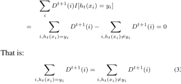
X i Dt+1(i)I[h t(xi) =yi] = X i,ht(xi)=yi Dt+1(i)− X i,ht(xi)6=yi Dt+1(i) = 0 That is: X i,ht(xi)=yi Dt+1(i) = X i,ht(xi)6=yi Dt+1(i) (33)
Hence, after weights being updated, weight distributions on misclassified samples and correctly classified samples get to even, i.e., T P = F P. This will make the learning of next iteration the most difficult [6].
By the weight update formula of AdaBoost.M1 (Equa-tion 13), weights of samples in two groups specified to class i, TP(i) and FP(i), updated from the tth iteration to the(t+ 1)thiteration can be summarized asT Pt+1(i) =
T Pt(i)/eαtandF Pt+1(i) =F Pt(i)·eαt. Withαtbeing a
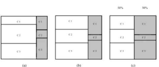
number of positive, identical for all classes, weights of false predictions (FP) are improved equally; weights of true pre-dictions (TP) are decreased equally, i.e., weighting scheme of AdaBoost.M1 treats samples of different classes equally. To illustrate this weighting effect, we take an example. Suppose we have a data set of three classes. The sam-ple distribution after a classification process is presented in Figure 2(a). The left side represents correctly classi-fied samples which occupy a larger proportion of the space
Figure 2. Resampling Effects of AdaBoost.M1
and the right side shaded represents samples mis-classified. On each side, samples are grouped by class labels, i.e., C1, C2 and C3. By weighting and normalizing of Ad-aBoost.M1, correctly classified space shrinks and misclas-sified space expands until these two parts get to equal. Fig-ure 2 (b) demonstrates this result. The notable point is on each part, correctly classified and misclassified, each group (class) shrinks or expands at the same ratio. Observa-tionally, the classes with relatively more misclassified sam-ples will get expanded, which are not necessary the classes we care about. To strengthen the learning on the “weak” classes, we expect more weighted sample sizes on them.
5.2
AdaC2.M1
The learning objective of AdaC2.M1 algorithm is to se-lectαtfor minimizingZton each round (Equation 30). The
first derivative ofZtas a function ofαtis
Z0t(α) = dZ dα = −X i ciDt(i)I[ht(xi) =yi]exp(−αtI[ht(xi) =yi]) = −Zt X i Dt+1(i)I[h t(xi) =yi]
by definition ofD(t+1)(Equation 26). To minimizeZt,αt
is selected such thatZ0(α) = 0. The unique solution for αtis presented by Equation 31. By the definition ofDt+1
(Equation 26), for the next iteration we will have
X
i,ht(xi)=yi
Dt+1(i) = X i,ht(xi)6=yi
Dt+1(i) (34)
It indicates that weight of the correctly classified group and that of the misclassified group get to even after sam-ple weights being updated by AdaC2.M1, i.e.,T P =F P. Same as AdaBoost.M1, this weighting result will make the learning of next iteration the most difficult.
By the weight update formula of AdaC2.M1( Equation 26), sample weights of two groups respecting to class i, T P(i) and F P(i), updated from the tth iteration to the (t+ 1)thiteration can be summarized asT P
t+1(i) =c(i)·
Figure 3. Resampling Effects of AdaC2.M1
T Pt(i)/eαtandF Pt+1(i) =c(i)·F Pt(i)·eαt. Wherec(i)
denotes the misclassification cost of classi. This weighting process can be interpreted in two steps. At the first step, each sample, no matter in which groups (TP or FP), is first weighted by its cost item (which equals to the misclassifica-tion cost of the class that the sample belongs to). Samples of the classes with larger cost values will obtain more sam-ple weights, on the other side, samsam-ples of the classes with smaller cost values will lose their sizes. Consequently, the class with the largest cost value will always enlarge its class size at this phase. The second step is actually the weighting procedure of AdaBoost.M1, i.e., weights of false predic-tions are expanded and those of true predicpredic-tions are shrunk. The expanding or shrinking ratio for samples of all classes is the same.
To demonstrate this weighting process, we use the same example as illustrated for AdaBoost.M1. In this case, we associate each class with a misclassification cost. Suppose the costs are 3, 1 and 2 respecting to classC1,C2andC3. Each sample obtains a cost value according to its class la-bel. Let the sample distribution after a classification process presented in Figure 3(a) be the same with that presented in Figure 2(a). By the weighting strategy of AdaC2.M1, the first step is to reweight each sample by its cost item. After normalizing, classes with relative larger cost values are ex-panded, oppositely, the other class is shrunk. In our exam-ple, class sizes of classC1andC3are increased and class size of classC2is decreased as presented in Figure 3 (b). At the next step, correctly classified space shrinks and mis-classified space expands until these two parts get to even. If we compare Figure 3(c) with Figure 2 (b), obviously, we can find out that classC1expands its class size updated by AdaC2.M1 more than that updated by AdaBoost.M1.
This observation shows that we can use the cost values to adjust the data distributions among classes. For those classes with poor performances, we can associate them with relative higher cost values such that relatively more weights are accumulated on those parts. As a result, learn-ing will bias and more relevant samples might be identi-fied. However, if weights are over boosted, more irrelevant samples can be included simultaneously. Precision values of these classes and recall values of the other classes will be decreased. Hence, how to figure out an efficient cost
setup which is able to yield satisfactory classification per-formance is the next problem to be solved.
6
Searching for an Optimum Cost Setup by
Genetic Algorithm
Genetic Algorithm (GA) is a directed random search technique invented by Holland [7]. It is based on the the-ory of natural selection and evolution. GA is a robust search method requiring little information to search in a large search space. Generally, GA requires two elements for a given application: 1) Encoding of candidate solutions; and 2) Fitness function for evaluating the relative perfor-mance of candidate solutions to identify the better one.
Genetic Algorithm codes candidate solutions of the search space as binary strings of fixed length. It employs a population of strings initialized at random, which evolve to the next generation by genetic operators such as selec-tion, crossover and mutation. The fitness function evalu-ates the quality of solutions. GA tends to take advantage of the fittest solutions by giving them greater weight, and concentrating the search in the regions which lead to better solutions of the problem. Therefore, GA searches through a population of points in contrast to the single point of focus of most other search algorithms, such as Simulated Anneal-ing and Hill ClimbAnneal-ing algorithms. Though it might not find the best solution, it would come up with a partially optimal solution.
In our case, we employ GA for searching an optimal misclassification cost setup, which will be applied to the AdaC2.M1 algorithm trying to improve the classification performance of the unbalanced data sets. Letc(i)denote the misclassification cost of classi. Then cost items ofkclasses making up a cost vector ofkelements[c(1)c(2) · · · c(k)] can be encoded as a binary string. The fitness value of each vector is the measurement of the classification performance when the vector is integrated in the AdaC2.M1 algorithm applied to a base classification system. Evaluation of the classification performance depends on the learning objec-tive. According to the learning objectives, the fitness func-tion is varied. The final output of GA is a vector that yields the most satisfactory classification performance among all tests.
7
Experiments
In this section, we set up experiments to investigate the cost-sensitive boosting algorithm AdaC2.M1 respecting to its capability in dealing with the class imbalance problem with multiple classes. For this purpose, we apply both Ad-aBoost.M1 and AdaC2.M1 to decision tree classification system C4.5 [17]. Then their performances on data sets
with multiple classes where the unbalanced class distribu-tions hinder the classification performances are compared and analyzed. Three data sets, Car data, New-thyroid data, and Nursery data, are taken from UCI Machine Learning Database [14] for our experiments.
7.1
Leaning Objectives and Evaluation
Measures
Refer to the confusion matrix of Table 1, the true pre-diction of theithclass is the number ofn
ii. Classification
accuracy is then calculated as: Accuracy= Pk i=1nii Pk i,j=1nij (35)
The evaluation measure of accuracy is inadequate in re-flecting the classifier’s performance on classifying each sin-gle class, especially on those small classes. The learning objective with unbalanced data with multiple classes can be either to improve the recognition success on a specific class or to balance identify ability over every classes. Respecting to the different learning objectives, the classification per-formance is evaluated by different measures. Regarding to classifying a single class, one should consider both its ability of recognizing available samples and the accuracy of recognizing relevant samples. These two aspects are re-ferred to asrecallandprecisionin information retrieval. Let Ri andPi denote recall and precision of class Ci
respec-tively, thenRiandPiare defined as:
Ri= Pknii j=1nij (36) and Pi=Pknii j=1nji (37)
Clearly neither of these measures are adequate by them-selves.F-measure(F) is suggested in [13] to integrate these two measures as an average:
Fi−measure= 2RiPi
Ri+Pi
(38)
It is obvious that if the F-measure is high when both the recall and precision should be high.
When the performances of all classes are interested, clas-sification performance of each class should be equally rep-resented in the evaluation measure. For the bi-class sce-nario, Kubat et al [12] suggested the G-mean as the geo-metric means of recall values of two classes. Expanding this measure to the multiple class scenario, we define G-mean as the geometric means of recall values of every classes:
G−mean= Ã k Y i=1 Ri !1/k (39)
As each recall value representing the classification perfor-mance of a specific class is equally accounted, G-mean is capable to measure the balanced performance among classes of a classification output.
Another often used method for evaluating classification of unbalanced data is ROC analysis [1]. A ROC graph depicts relative trade-offs between true positives and false positives within the bi-class concepts. The ROC analysis method needs a classifier to yield a score representing the degree to which an example pertaining to a class. In this study, we will evaluate our experimental performances by F-measure and G-mean.
7.2
Experiment Method
For each data set, available samples are used for both cost setup searching and performance evaluation. For this purpose, we carry on two sections of partitions. The first section of partitions is for searching cost setups by GA. The data set is randomly divided into two sets:80%as the train-ing set and the remaintrain-ing20%as the validation set for mea-suring the goodness of a bunch of cost setups generated by GA. The out put is a cost vector which obtains the best fit-ness value among all tests. This process is repeated 20 times such that one prototype is obtained from a pool of 20 cost vectors. The second section of partitions, totally indepen-dent from the first section, is for evaluating the classifica-tion performance. The whole data set is reparticlassifica-tioned into two sets:80%as the training set and the remaining20%as the test set. This process is repeated 10 times to obtain an average performance. For a consistent comparison, classifi-cation models of C4.5, C4.5 applied by AdaBoost.M1 and C4.5 applied by AdaC2.M2 are trained and evaluated with same data partitions.
The cost setup used by AdaC2.M2 is the prototype from the validation tests with the first section of partitions. In our experiments, we take the mean of a pool of 20 cost vectors as the cost setup prototype. As stated in [3], given a set of cost setups, the decisions are unchanged if each one in the set is multiplied by a positive constant or added with a con-stant. The ratios among cost values denote the deviations of the leaning importance among classes. Therefore, normal-izing each cost vector in the pool is a necessary step before calculating the mean value. The normalization method is, first, to set the value of the element with the maximum value in a vector as 1, then, to scale other elements’ values in the vector with the ratio of 1 over the maximum value. After normalizing of each cost vector, a mean is calculated as the prototype. The prototype vector is also normalized before
putting it in use for further experiments.
7.3
Car Evaluation Database
This database was derived for car evaluating. There are 1728 instances with each is described by 6 nominal ordered attributes. The whole data are grouped into 4 classes. Table 2 describes the class distribution.
Table 2. Class Distribution
index class name class size class distribution
C1 unacc 1210 70.023%
C2 acc 384 22.222%
C3 good 69 3.993%
C4 v-good 65 3.762%
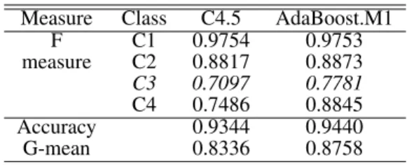
Class C3 and C4 are two small classes which posses only 3.993%and 3.762% samples respectively. We first use the second section of data partitions to test the per-formance of C4.5 and C4.5 applied by AdaBoost.M1. For this part of experiments, the classification performance are recorded respecting to both each individual class and the overall performance. Respecting to each class F-measure value (Equation 38) is calculated. Respecting to the over-all performance, both classification accuracy (Equation 35) and G-mean (Equation 39) are reported. Experiment results are tabulated in Table 3.
Table 3. Performance of C4.5 & AdaBoost.M1
Measure Class C4.5 AdaBoost.M1
F C1 0.9754 0.9753 measure C2 0.8817 0.8873 C3 0.7097 0.7781 C4 0.7486 0.8845 Accuracy 0.9344 0.9440 G-mean 0.8336 0.8758
Respecting to the classification of C4.5, performances of classes C1 and C2 are significantly better than those of class C3 and C4, which are two small classes. By apply-ing AdaBoost.M1, performances of class C1 and C2 remain similar values; that of class C4 is significantly improved; performance of class C3 is also improved but far behind other classes’. As for the overall performance, classifica-tion accuracy of C4.5 is improved slightly; G-mean value is improved by 4.22% by applying AdaBoost.M1. Based on these observations, for testing AdaC2.M1 we set up two learning objectives: 1) to further balance the identify ability on each class; and 2) to improve the recognition ability of class C3. We then run GA for searching an efficient cost setup with data partitions of the first section.
Respecting to the first learning objective, the fitness function is G-mean evaluation. The resulting prototype of a cost vector is[0.3281 0.6682 0.7849 1.0000]. Integrating this cost vector into AdaC2.M1, classification performances are evaluated by G-mean on the data partitions of the second section such that C4.5, C4.5 applied by AdaBoost.M1, and C4.5 applied by AdaC2.M1 are evaluated on the same train-ing and test partitions. Table 4 tabulates results for compar-isons.
Table 4. G-mean Evaluation
Class C4.5 AdaBoost.M1 AdaC2.M1
C1(R) 0.9637 0.9707 0.9586
C2(R) 0.9083 0.9056 0.9459
C3(R) 0.7175 0.7395 0.8540
C4(R) 0.7902 0.9151 0.9139
G-mean 0.8336 0.8758 0.9146
As G-mean is calculated as the geometric means of re-call values of every classes, each row indicated by class la-bel in Table 4 are the recall values achieved by C4.5, C4.5 applied by AdaBoost.M1, and C4.5 applied by AdaC2.M1 respectively and the row indicated by “G-mean” are those G-mean values. Respecting to the two small classes C3 and C4, recall value of C4 is improved and that of C3 fails to be improved by AdaBoost.M1. By applying AdaC2.M1, recall value of C3 is greatly improved. In general, G-mean value of C4.5 is increased by4.22% by applying AdaBoost.M1 and by8.10% by applying AdaC2.M1, which obtains the highest G-mean values through increasing recall values of both classes C3 and C4.
Respecting to the second learning objective, the fitness function is the F-measure evaluation of class C3. The result-ing prototype cost vector is[0.5412 0.8217 0.7536 1.0000]. Integrating this cost vector to AdaC2.M1, classification per-formance of class C3 is evaluated by the data partitions of the second section. Table 5 presents the performances of C4.5, AdaBoost and AdaC2.M1 including recall (R), preci-sion (P) and F-measure (F) values of class C3. F-measure value of C4.5 is improved by AdaBoost.M1 through in-creasing the precision value. By applying AdaC2.M1, both recall and precision values are improved and keep relatively even. AdaC2.M1 hence achieves the best F-measure value.
Table 5. F-measure Evaluation on Class C3
C4.5 AdaBoost.M1 AdaC2.M1
R 0.7175 0.7395 0.8364
P 0.7068 0.8389 0.8289
F 0.7097 0.7781 0.8304
7.4
New-Thyroid Database
The goal of this data set is to predict a patient’s thyroid to the class euthyroidism (normal), hypothyroidism or hyper-thyroidism. This data is a simple database containing 215 instances of patients, each described by 5 attributes. Table 6 describes the class distribution.
Table 6. Class Distribution
index class name class size class distribution
C1 normal 150 69.77%
C2 hyper 35 16.28%
C3 hypo 30 13.95%
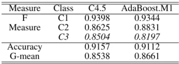
Two classes of this data set, C2 and C3, are small classes. By the same experiment method as described previously for the Car data, we first test C4.5 and C4.5 applied by Ad-aBoost.M1. Experiment results are tabulated in Table 7.
Table 7. Performance of C4.5 & AdaBoost.M1
Measure Class C4.5 AdaBoost.M1
F C1 0.9398 0.9344
Measure C2 0.8625 0.8831
C3 0.8504 0.8197
Accuracy 0.9157 0.9112
G-mean 0.8538 0.8661
Respecting to classification performance of C4.5, per-formance on class C1 is significantly better than the other two small classes C2 and C3. By applying AdaBoost.M1, performance of class C1 remains the similar value; that of class C2 is improved by 2.06%; and that of class C3 is decreased by3.13%; Classification accuracy of C4.5 does not change a lot and G-mean value is slightly improved by 1.23%. Based on these observations, we set up two learning objectives: 1) to further balance the identify ability on each class; and 2) to improve the recognition ability of class C3. Respecting to the first learning objective, the fitness function is G-mean evaluation. The resulting prototype of a cost vector is [0.4206 0.6256 1.0000]. Integrating this cost vector into AdaC2.M1, classification performance of each individual class reported by recall value and the over-all performance evaluated by G-mean, together with those yielded by C4.5 and C4.5 applied by AdaBoost.M1 are tab-ulated in Table 8. Recall value of class C1 is decreased by both AdaBoost.M1 and AdaC2.M1, but still keeps a good performance. Recall value of C2 is increased by 5.84% through applying Adaboost.M1 and by9.49%through ap-plying AdaC2.M1. For the class C3, recall value of C4.5 fails to be improved by AdaBoost.M1 and is increased
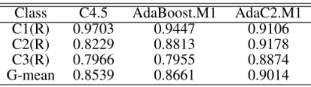
by9.08%through applying AdaC2.M1. G-mean value of C4.5 is slightly improved by applying AdaBoost.M1 and significantly improved by 5.75% by applying AdaC2.M1. AdaC2.M1 achieves the best G-mean value by increasing recall values of both classes C2 and C3.
Table 8. G-mean Evaluation
Class C4.5 AdaBoost.M1 AdaC2.M1
C1(R) 0.9703 0.9447 0.9106
C2(R) 0.8229 0.8813 0.9178
C3(R) 0.7966 0.7955 0.8874
G-mean 0.8539 0.8661 0.9014
Respecting to the second learning objective, the fitness function is the F-measure evaluation of class C3. The re-sulting prototype cost vector is[0.7697 0.9804 1.0000]. In-tegrating this cost vector into AdaC2.M1, classification per-formance of class C3 together with those of C4.5 and C4.5 applied by AdaBoost.M1 are stated in Table 9. The F-measure performance of C4.5 is decreased by applying Ad-aBoost.M1 since the recall value is not changed a lot and precision value is lowered. By applying AdaC2.M1, recall value is increased and precision value is lowered such that these two values get closer. The resulting F-measure value obtained by AdaC2.M1 is a little bit better than that of C4.5.
Table 9. F-measure Evaluation on Class C3
C4.5 AdaBoost.M1 AdaC2.M1
R 0.7966 0.7955 0.8763
P 0.9467 0.8574 0.8547
F 0.8504 0.8197 0.8613
7.5
Nursery Database
Nursery Database was derived to rank applications for nursery schools. There are 12960 instances, each described by 8 nominal attributes. The original data has 5 classes. Since one class, “recommend”, has only 2 instances, we therefore combine this class with class “very-recommend”. Table 10 describes the class distribution.
Table 10. Class Distribution
index class name class size class distribution
C1 not-recom 4320 33.33%
C2 very-recom 330 2.55%
C3 priority 4266 32.92%
C4 spec-prior 4044 31.20%
With this data set, class C2 is the only small class. Ex-periment results of C4.5 and C4.5 applied by AdaBoost.M1. are tabulated in Table 11.
Table 11. Performance of C4.5 & Ad-aBoost.M1
Measure Class C4.5 AdaBoost.M1
F C1 1 1 Measure C2 0.7784 0.8992 C3 0.9617 0.9829 C4 0.9765 0.9895 Accuracy 0.9747 0.9887 G-mean 0.9250 0.9625
Obviously, performance of class C2 is the worst among these 4 classes by both C4.5 and AdaBoost.M1, even thought it is improved by applying AdaBoost.M1. Classifi-cation accuracy and G-mean value of C4.5 are improved by applying AdaBoost.M1. We set up two learning objectives: 1) to further balance the identify ability on each class; and 2) to improve the recognition ability of class C2.
Respecting to the first learning objective, the fitness function is G-mean evaluation. The resulting prototype of a cost vector is[0.7072 1 0.4888 0.6516]. Integrating this cost vector into AdaC2.M1, classification recall value of each individual class and the G-mean value, together with those generated by C4.5 and C4.5 applied by Ad-aBoost.M1 are tabulated in Table 12. Respecting to class C2, recall value is increased by10.40% through applying AdaBoost.M1 and by15.68%through applying AdaC2.M1. The G-mean value achieved by C4.5 is increased by3.75% through applying AdaBoost.M1 and by4.95%through ap-plying AdaC2.M1. Both improvements are achieved mainly through increasing the recall value of class C2.
Table 12. G-mean Evaluation
Class C4.5 AdaBoost.M1 AdaC2.M1
C1(R) 1 1 1
C2(R) 0.7776 0.8816 0.9344
C3(R) 0.9630 0.9851 0.9755
C4(R) 0.9750 0.9889 0.9906
G-mean 0.9250 0.9625 0.9745
Respecting to the second learning objective, the fitness function is the F-measure evaluation of class C2. The re-sulting prototype cost vector is[0.7131 1 0.5310 0.2895]. Integrating this cost vector into AdaC2.M1, classification performance of class C2 together with those of C4.5 and C4.5 applied by AdaBoost.M1 are stated in Table 13. By applying AdaBoost.M1, F-measure value of C4.5 is signif-icantly improved, from77.84%to89.92%. Both recall and
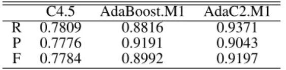
precision values are increased simultaneously. By apply-ing AdaC2.M1, recall value is further improved and pre-cision value is slightly decreased comparing with that of AdaBoost.M1. The combination evaluation F-measure of AdaC2.M1 is better than that of AdaBoost.M1.
Table 13. F-measure Evaluation on Class C3
C4.5 AdaBoost.M1 AdaC2.M1
R 0.7809 0.8816 0.9371
P 0.7776 0.9191 0.9043
F 0.7784 0.8992 0.9197
8
Conclusion
In this paper, we developed a cost-sensitive boosting al-gorithm AdaC2.M1 to tackle the class imbalance problem with multiple classes (more than two classes). The main contributions of this research are: 1) to the best of our knowledge, this is the first work to address the class im-balance problem involving multiple classes. The signifi-cant hardness and importance in solving the class imbal-ance problem attracts a lot of research interests. However, most the existing approaches assume a bi-class setting. Due to the complicated situations when multiple classes present, methods for bi-class problems are not directly applicable; 2) the AdaC2.M1 algorithm has been developed by reducing its weight update parameter to minimize the overall train-ing error of the combined classifier taktrain-ing the misclassifi-cation costs into consideration. This process is crucial for the boosting efficiency; 3) our study shows that AdaC2.M1 is capable to adjust the data distributions and bias the lean-ing focuses among classes by settlean-ing up different cost val-ues; and 4) we set up efficient cost vectors for apply-ing AdaC2.M1 by the searchapply-ing of the Genetic Algorithm. Conducted experimental tests on three “real world” data sets indicate that, with the searching results of GA, AdaC2.M1 is capable to improve the base classification’s performances and accomplish better results than AdaBoost.M1 when both boosting algorithms are applied to the C4.5 classification systems. Due to the nature of GA, searching of cost setups might be time-consuming with some applications. This ap-proach is still respectable considering that this searching is usually an off-line procedure such that the learning speed is not a crucial issue.
References
[1] A. P. Bradley. The use of the area under the ROC curve in the evaluation of machine learning algorithms. Pattern Recognition, 30(7):1145–1159, 1997.
[2] N. Chawla, N. Japkowicz, and A. Kolcz. Editorial: Special issue on learning from imbalanced data sets. SIGKDD Explorations Special Issue on Learning from Imbalanced Datasets, 6(1):1–6, 2004.
[3] C. Elkan. The foundations of cost-sensitive learning. In Proceed-ings of the Seventeenth International Joint Conference on Artificial Intelligence, pages 973–978, Seattle, Washington, August 2001. [4] W. Fan, S. J. Stolfo, J. Zhang, and P. K. Chan.
Ada-cost:misclasification cost-sensitive boosting. InProceedings of Sixth International Conference on Machine Learning(ICML-99), pages 97–105, Bled, Slovenia, 1999.
[5] Y. Freund and R. E. Schapire. A decision-theoretic generalization of on-line learning and an aplication to boosting.Journal of Computer and System Sciences, 55(1):119–139, August 1997.
[6] J. Friedman, T. Hastie, and R. Tibshirani. Additive logistic regres-sion: a statistical view of boosting.Annals of Statistics, 28(2):337– 374, April 2000.
[7] J. H. Holland.Adaptation in Natural and Artificial Systems. Univer-sity of Michigan Press, Ann Arbor, MI, 1975.
[8] N. Japkowicz. Supervised versus unsupervised binary-learning by feedforward neural networks.Machine Learning, 41(1), 2001. [9] N. Japkowicz and S. Stephen. The class imbalance problem: A
sys-tematic study.Intelligent Data Analysis Journal, 6(5):429–450, No-vember 2002.
[10] M. V. Joshi.Learning Classifier Models for Predicting Rare Phone-mena. PhD thesis, University of Minnesota, Twin Cites, Minnesota, USA, 2002.
[11] M. V. Joshi, V. Kumar, and R. C. Agarwal. Evaluating boosting al-gorithms to classify rare classes: Comparison and improvements. In
Proceeding of the First IEEE International Conference on Data Min-ing(ICDM’01), 2001.
[12] M. Kubat, R. Holte, and S. Matwin. Machine learning for the detec-tion of oil spills in satellite radar images.Machine Learning, 30:195– 215, 1998.
[13] D. Lewis and W. Gale. Training text classifiers by uncertainty sam-pling. InProceedings of the Seventeenth Annual International ACM SIGIR Conference on Research and Development in Information, pages 73–79, New York, NY, August 1998.
[14] P. M. Murph and D. W. Aha. UCI Repository Of Machine Learning Databases. Dept. Of Information and Computer Science, Univ. Of California: Irvine, 1991.
[15] M. Pazzani, C. Merz, P. Murphy, K. Ali, T. Hume, and C. Brunk. Reducing misclassification costs. InProceedings of the Eleventh In-ternational Conference on Machine Learning, pages 217–225, New Brunswick, NJ, July 1994.
[16] F. Provost and T. Fawcett. Analysis and visualization of classifier per-formance: Comparison under imprecise class and cost distributions. InProceedings of the Third International Conference on Knowledge Discovery and Data Mining (KDD-97), pages 43–48, Newportbeach, CA, August 1997.
[17] J. R. Quinlan.C4.5: programs for machine learning. Morgan Kauf-mann Publishers, 1993.
[18] R. E. Schapire and Y. Singer. Boosting the margin: A new expla-nation for the effectiveness of voting methods. Machine Learning, 37(3):297–336, 1999.
[19] R. E. Schapire and Y. Singer. Improved boosting algorithms us-ing confidence-rated predictions.Machine Learning, 37(3):297–336, 1999.
[20] Y. Sun, A. K. C. Wong, and Y. Wang. Parameter inference of cost-sensitive boosting algorithms. InProceedings of 4th International Conference on Machine Learning and Data Mining in Pattern Recog-nition, pages 21–30, Leipzig, Germany, July 2005.
[21] K. M. Ting. A comparative study of cost-sensitive boosting algo-rithms. InProceedings of the 17th International Conference on Ma-chine Learning, pages 983–990, Stanford University, CA, 2000. [22] K. M. Ting. An instance-weighting method to induce cost-sensitive
trees. IEEE Transaction on Knowledge and Data Engineering, 14(3):659–665, 2002.
[23] G. Weiss. Mining with rarity: A unifying framework. SIGKDD Explorations Special Issue on Learning from Imbalanced Datasets, 6(1):7–19, 2004.
[24] G. Weiss and F. Provost. Learning when training data are costly: The effect of class distribution on tree induction. Journal of Artificial Intelligence Research, 19:315–354, 2003.