Prediction of Polycomb/Trithorax Response Elements using Support Vector Machines

(1)

Prediction of Polycomb/Trithorax Response Elements using

Support Vector Machines

Bjørn Andr´e Bredesen

Master’s thesis

Department of Informatics

University of Bergen

(2)

i

Abstract

Polycomb/Trithorax Response Elements (PREs) are epigenetic elements that can maintain established tran-scriptional states over multiple cell divisions. Sequence motifs in known PREs have enabled genome-wide PRE prediction by the PREdictor and jPREdictor, using combined motif occurrences for scoring sequence windows. The EpiPredictor predicts PREs by using the method of Support Vector Machines (SVM), which enables the construction of non-linear classifiers by use of kernel functions. Aspects of using SVMs for PRE prediction can be investigated, such as setting of SVM parameters, using SVM decision values for scoring and using alternative feature sets.

The PRE prediction implementation presented in this thesis, called PRESVM, uses SVM decision values to score sequence windows. PRESVM implements the feature sets used by (j)PREdictor and EpiPredictor, as well as feature sets using relative motif occurrence distances and periodic motif occurrence. Grid search and Particle Swarm Optimization are supported for setting SVM parameters. For evaluating PRE predictions of multiple classifiers against experimental data sets, an application called PREsent has been implemented.

For a similar configuration for PRESVM and jPREdictor, PRESVM predicted a larger number of can-didate PREs, which were more sensitive to but had lower Positive Predictive Values against experimental data considered than those of jPREdictor. A formal relationship was established between the PRESVM and jPREdictor decision functions for this configuration. The trade-offs make it difficult to conclude that either classifier is superior. Many configurations remain to be tested, and the results encourage further testing.

(3)

ii

Acknowledgements

First, I would like to thank Marc Rehmsmeier (University of Bergen, Department of Informatics) for his su-pervision of the work with this thesis, with regular meetings with helpful and inspiring discussions. I would also like to thank Marc Rehmsmeier for proposing this project to me and thus introducing me to the exciting field of Polycomb epigenetics and the application of machine learning to genome-wide search.

I would like to thank Takaya Saito and Ksenia Lavrichenko in the Rehmsmeier group (University of Bergen, Department of Informatics) for sharing office with me and for friendly conversations.

I would also like to thank my younger brother, Marius Bredesen, with whom I have lived during my master’s degree studies, and with whom I have had many inspiring conversations.

(4)

Contents iii

5.2 PRESVM . . . 21

5.3 Support Vector Machines and sequences . . . 22

5.4 Training data . . . 23

5.5 Genome-wide prediction . . . 24

5.6 Classifier threshold calibration . . . 24

5.7 Comparison of PRESVM and other PRE prediction methods . . . 28

6 Sequence features 31 6.1 Motif occurrence frequency features . . . 31

6.2 Motif occurrence distance features . . . 34

6.3 Periodic motif occurrence frequency features . . . 36

6.4 Other motif occurrence features . . . 38

6.5 Other sequence features . . . 39

7 Configuration optimization 40 7.1 Configuration vectors . . . 40

7.2 Grid search . . . 40

7.3 Approximated gradient search . . . 41

7.4 Particle Swarm Optimization . . . 44

(5)

Contents iv

8 Validation of Polycomb/Trithorax Response Element predictions 47

8.1 Validating predicted PRE regions . . . 47

8.2 Predicting and validating PcG target genes . . . 48

8.3 PREsent . . . 49

8.4 Genome-wide validation plots . . . 49

8.5 Comparing against multiple data sets . . . 50

9 Results 51 9.1 Tests of PRESVM configurations . . . 51

9.2 Genome-wide prediction with PRESVM . . . 53

9.3 Comparison with the jPREdictor . . . 58

9.4 Interpretations of results . . . 58

10 Implementation 66 10.1 PRESVM implementation . . . 66

10.2 Sequence reading . . . 66

10.3 Motif occurrence parsing . . . 67

10.4 Motif occurrence handling . . . 69

10.5 PREsent implementation . . . 69 10.6 Other implementations . . . 72 11 Discussion 73 11.1 Conclusion . . . 73 11.2 Future work . . . 74 List of Figures 75 List of Tables 77 List of Algorithms 79 List of Definitions 80 Notation overview 82 Bibliography 84

(6)

Chapter 1. Preface 1

Chapter 1

Preface

The project for this thesis was proposed by Marc Rehmsmeier, my supervisor during my master’s degree stud-ies. Marc Rehmsmeier has worked with Leonie Ringrose onin silicoprediction of instances of a type of DNA sequence element called Polycomb/Trithorax Response Elements (PREs for short). In this thesis, work con-tinues on this task by applying a different method, the machine learning method of Support Vector Machines. There are DNA sequences of known PREs, but what defines them is not well understood. The method Ringroseet al. [1] developed made use of pairing certain sequence motifs (short re-occurring substrings) in the known PREs, and they found that this better distinguished PREs from non-PREs than considering the motifs by themselves [1]. The machine learning method of Support Vector Machines enables modelling non-linear relationships, and the work by Ringrose et al. would suggests that non-linear relationships between motif occurrences could play a role. It is thus interesting to ask whether using Support Vector Machines might improve PRE prediction.

Soon after having started with this master’s project, an article was published by Zenget al. [2] in which Support Vector Machines were used for predicting PREs. However, multiple aspects of using Support Vector Machines for PRE prediction were not discussed. In this thesis, the use of Support Vector Machines for predicting PREs is explored further.

In Chapters 2-4, the background will be given. First, the biology of Polycomb/Trithorax Response El-ements will be discussed. Afterwards, machine learning and Support Vector Machines will be explained. Then, the considered statistics for evaluating results will be given.

In Chapter 5, the method used in this thesis is outlined, and Chapter 6 and Chapter 7 elaborate on details of the method. Multiple parts of the method are based on the method developed by Ringroseet al. [1]. However, the use of Support Vector Machines has its own considerations to make, and these will be discussed. Also, Support Vector Machines are flexible, and making use of this flexibility will be explored.

It is important to evaluate how well the prediction results obtained using the method agree with exper-imental results. Chapter 8 outlines how such evaluations can be made. Results are presented in Chapter 9, including tests of some of the possibilities that the method of Support Vector Machines offers, as well as comparison with the method developed by Ringroseet al. [1].

Two main software applications have been developed during the work with this thesis, and their imple-mentations are the subject of Chapter 10.

(7)

Chapter 2. Biological background 2

Chapter 2

Biological background

Inside the nucleus of eukaryotic cells, hereditary information is stored in chromosomes as sequences of de-oxyribonucleotides (DNA). In prokaryotic cells, hereditary information is stored as DNA in the nucleoid. The DNA sequence of all chromosomes of a cell constitute its genome. Reading DNA sequences from DNA molecules is called sequencing. Today, multiple genomes have been sequenced. In this thesis, the focus is on the genome of the fruit fly,Drosophila melanogaster.

2.1

The Polycomb system

The Drosophila melanogaster genome contains over 120 million base pairs, divided on chromosomes X/Y, 2L/2R, 3L/3R and 4. The genome contains regions that encode functional products such as proteins, called genes [3], as well as regions with other functions. The FlyBase [4]Drosophila melanogasterannotation release 5.47 contains over fifteen thousand annotated genes. According to the central dogma of molecular biology, the genes are transcribed from DNA to messenger RNA, which in turn is translated to protein [5]. The transcription of genes to RNA is referred to as gene expression [3]. The genome is largely the same in all cells of an organism, but cells need the ability to specialize to perform particular functions in a multi-cellular organism. Thus, there is a need for regulating the expression of genes. It may also be necessary for cells to be able to remember gene expression states over cell division. The persistence of the expression states of genes over cell division, not caused by a change in the genomic sequence, nor by the event that established the expression states, is called epigenetics [6].

InDrosophila melanogaster, two types of genomic elements that are involved in regulating the expression of genes are called initiator elements, which are involved in establishing states of gene transcription, and maintenance elements, which maintain established gene transcription states [6].

Polycomb/Trithorax Response Elements (or PREs for short), the sequence elements that are investigated in this thesis, are maintenance elements. Polycomb group (PcG) and Trithorax group (TrxG) proteins asso-ciate with this class of cis-regulatory DNA elements (regulating on the same DNA molecule), and through the PREs they can maintain established transcriptional states over many cell generations, making the PREs epigenetic [6]. The roles of the PcG and TrxG proteins in PRE target gene expression state maintenance are antagonistic, where PcG proteins maintain transcriptional repression, whereas TrxG proteins maintain active transcriptional states [6].

On the PREs, PcG and TrxG proteins form complexes [7]. Currently, three PcG protein complexes have been identified inDrosophila melanogaster, called Polycomb Repressive Complexes 1 (PRC1) and 2 (PRC2), and Pleiohomeotic Repressive Complex (PhoRC) [7]. The PcG proteins at the core of these complexes are listed in Table 2.1. Of the PcG proteins, Pho binds to specific DNA sequences, and additional proteins that bind to PREs may be involved in the recruitment of the PcG complexes [7]. In addition toDrosophila melanogaster, there is also work on PcG proteins in vertebrates, where their involvement includes cancer and

(8)

maintaining stem cell and differentiated cell identity [8].

2.2

Determination of Polycomb/Trithorax Response Elements

Multiple methods have been employed in the search for Polycomb/Trithorax Response Elements. Early methods include transgene analysis and chromatin immunoprecipitation (ChIP) [1]. In recent years, multiple new methods have aided in the discovery of PREs. In 2003, Ringrose et al. [1] devised a computational procedure called the PREdictor, which enabled in silico prediction of PREs across the whole Drosophila melanogaster genome (genome-wide). Since then, the ChIP-chip (ChIP combined with microarray [9]) and ChIP-seq (ChIP combined with high-throughput sequencing [10]) methods have been developed and applied for discovering PREs and their associated target genes [11, 12, 13, 14, 15].

With the PREdictor, Ringroseet al. [1] used sequences of known 12 PREs and 16 non-PREs to predict PREs genome-wide. The 12 PRE sequences have lengths ranging from 1219bpto 5383bp, and the 16 non-PRE sequences have lengths ranging from 369bpto 7008bp. Alignment of the known PRE sequences has shown little sequence similarity, but these sequences are enriched in certain sequence motifs [1]. Sequence motifs are short, re-occurring strings of DNA. They may be degenerate, meaning that for some motif positions, multiple nucleotides might be accepted, and mismatches may also be accepted. Ringroseet al. [1] considered 7 sequence motifs, and these are listed in Table 2.2. Most of these correspond to PcG/TrxG protein binding sites [1].

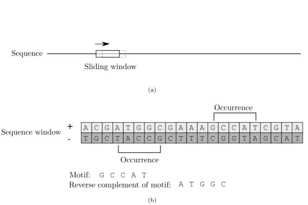
The PREdictor scans the PRE and non-PRE sequences for occurrences of 7 sequence motifs and their re-verse complements (corresponding to occurring on the opposite strand) (Figure 2.1(b)). Weights are assigned to the motifs or pairs of motifs according to how often they occur in the PRE versus non-PRE sequences, and this is used to assign scores to sequence windows. For evaluation, a 500bp sliding window is moved in 100bpincrements across the PRE and non-PRE sequences (Figure 2.1(a)), the corresponding regions are scored, and the maximum window score obtained for each sequence is considered. Ringrose et al. [1] found that scores based on occurrence frequencies of individual motifs only weakly separate PREs from non-PREs. Ringroseet al. [1] then considered the frequencies with which pairs of the 7 motifs occur within 220bpfrom each other in PRE versus non-PRE sequences, and they found that these give better separation of PREs from non-PREs. The next step in their method establishes a score cutoff such that only one region is expected to have a higher score than the cutoff in a randomly generated sequence of the same length as and with the nucleotide distribution of theDrosophila melanogaster genome. The PREdictor was then applied across the Drosophilagenome, which resulted in the prediction of 167 non-overlapping PREs. Multiple of the predicted PREs have been verified [16].

ChIP allows investigating the association between certain proteins and DNA [17]. This is done by cross-linking the proteins of interest and DNA. The sequence is then be split at random points (ideally uniformly), and the sequence fragments that are cross-linked to the protein of interest are isolated. The remaining se-quence fragments are then treated with a micro-array (ChIP-chip [9]) or sese-quenced (ChIP-seq [10]). These methods have been applied in a number of studies, for genome-wide mapping of the binding of PcG and TrxG proteins to identify PREs and associated target genes [11, 12, 13, 14, 15].

Work on computational determination of PREs has since continued. In 2006, a new, versatile implemen-tation of PREdictor, called the jPREdictor, was implemented in Java, containing a Graphical User Interface (GUI) and support for Position-Specific Scoring Matrix (PSSM) motifs [18]. Fiedler and Rehmsmeier [18] tested PRE prediction with the jPREdictor with the addition of a PSSM Pho motif and the DSP1 motif, which resulted in 378 PRE predictions. Additional motifs have since been discovered, and these are listed together with the DSP1 motif in Table 2.3. However, training the jPREdictor with the addition of the rest of these motifs did not result in improved PRE prediction [19]. In 2012, Zenget al. devised the EpiPredictor [2], a Support Vector Machine PRE prediction method, in which the occurrence frequencies of the 7 se-quence motifs considered by Ringroseet al. were used. In 2013, a Support Vector Machine PcG target gene

(9)

Complex Core proteins PRC1

Polyhomeotic (Ph) Posterior sex combs (Psc) Sex combs extra (Sce) Polycomb (Pc) PRC2

Enhancer of zeste (E(z)) Supressor of zeste 12 (Su(z)12) Nurf55

PhoRC

Pleiohomeotic (Pho) dSfmbt

Table 2.1: Core proteins of the PcG complexes of Drosophila melanogaster that have been characterized [7].

(a)

+

-A C G -A T G G C G -A -A -A G C C -A T C G T -A T G C T A C C G C T T T C G G T A G C A T G C C A T A T G G C (b)

Figure 2.1: 2.1(a): A sliding window moves across the sequence in fixed increments. 2.1(b) Motif occurrences or their reverse complements are found.

(10)

Name Function Sequence motif Allowed number

of mismatches

G GAGA factor (GAF) binding site GAGAG 0

G10 Extended GAGA factor (GAF) binding site GAGAGAGAGA 1 PS Pleiohomeotic (Pho/Phol) core site GCCAT 0 PM Pleiohomeotic (Pho/Phol) consensus CNGCCATNDNND 0 PF Pleiohomeotic (Pho/Phol) consensus GCCATHWY 0 EN 1 Motif important forengrailed PRE silencing GSNMACGCCCC 1

Z Zeste binding site YGAGYG 0

Table 2.2: These sequence motifs were used by Ringroseet al. [1] for predicting Polycomb/Trithorax Response Elements with the PREdictor. The motif sequences are given in IUPAC nucleotide codes.

Binding protein Sequence motif

Dsp1 GAAAA

Grainy head (Grh) TGTTTTT

Sp1/KLF RRGGYGY

Table 2.3: Since the original work of Ringroseet al. with the PREdictor, these motifs have been discovered [6]. The motif sequences are given in IUPAC nucleotide codes.

prediction method was devised that does not require a negative training set, using Mapping-Convergence [20]. In this thesis, the work continues onin silico PRE identification. Machine learning is central to this work, and is discussed in the next chapter.

(11)

Chapter 3. Machine learning 6

Chapter 3

Machine learning

For many tasks, it can be difficult to formulate a particular algorithm that may perform the task well. The task might be poorly understood, and the system might need the ability to adapt to new information. One may, however, be able to formulate the problem in terms of experiences, such that if the system could learn from those experiences, the system would be able to perform the task.

Machine learning enables the construction of systems that can learn. Machine learning is applied to many different problem areas. Examples include problems of constructing systems producing advanced behaviours, such as robot control and playing games, and recognition and prediction problems. For the former type of problems, the system may learn from experimentation. For the latter, one typically selects examples for the system to learn from, and it may then be implemented as a classification problem. In this thesis, machine learning is used for classification.

3.1

Classification problems and learning

In classification problems, one has a set of objects, X, and a set of classes, C ={C1, ..., Cn}. The task is

to decide which class Ci an object x ∈ X is an instance of. If there are two classes, this is called binary

classification.

Definition 1 (Classifier) For a set of objects X and a set of classes C = {C1, ..., Cn}, a classifier is a

function c : X → C, which assigns classes Ci to objects x ∈ X. A decision function will here refer to a

functional formulation of a classifier.

Learning comes in when the correct definition of the classifierc(x) is unknown, but classes are known for a subset of objects. It is then desirable to construct an approximation ofc(x) based on a set of objects with known classes.

Definition 2 (Function approximation) A hat over a function name will be used to denote an approxi-mately equal function, i.e. ˆc(x)≈c(x).

Definition 3 (Cartesian product) For two sets X andY,X ×Y ={(x, y)|x∈X∧y∈Y} denotes the Cartesian product.

Definition 4 (Training set) A training set is a set that will be presented to a learning machine. For using objects from a set X with known classes, it will be a set T ⊂X ×C of pairs of objects and known classes. The elements(x, y)∈T will be referred to as training examples.

Elements of a training set (x, y) ∈ T may be presented to a learning machine. The learning machine constructs an approximation ˆc(x) ≈c(x) =y, which may be used to classify objects for which the correct class is not known a priori. This is an example of supervised machine learning, since the objects in the training set are labelled with classes (the alternative is called unsupervised learning). Supervised machine learning is often used for learning concepts, where the goal is to predict members versus non-members of a

(12)

concept. This can be implemented as a binary classification.

A machine learning method needs to store the knowledge that is to be learned. This storage will typically be in a form that makes generalizing assumptions about the relationships between the training examples that have been presented. This results in a model, and the process of generating or updating the model based on examples is called learning. The generalizing assumptions make it possible to use the resulting model for making predictions outside the training set.

Definition 5 (Model) An approximation c(x)ˆ ≈c(x) generated by a machine learning method will be re-ferred to as a model.

Definition 6 (Learning) The process of generating and updating a model based on training examples will be referred to as learning.

The objects x ∈ X may not be of a type readily useable by a machine learning method. It is then necessary to extractfeatures from the objects that can be presented to the learning machine.

Definition 7 (Feature) A featuref(x)of an objectx∈X is a description of a property ofx. In this thesis, such a property description will always be a real value, i.e. f :X →R.

Definition 8 (Vector) A vector~a∈Rd is a vector of real values (a1, a2, ..., ad).

If the objects are strings of text, the features can for example be the frequencies with which particular words occur within the objects. For an object x, the word frequencies might then be collected into a vector of real values~xand presented to the learning machine.

When applying machine learning to a classification problem, it is important to select a good training set and feature set. The features should be sufficiently descriptive of the objects belonging to each class, and the training set should contain objects that sufficiently represent the classes.

Ideally, the resulting model should generalize to the largerX×C,i.e. ˆc(x)≈c(x),∀x∈X. If the learning machine learns the training set too well, it may be biased by the choice of training set, which can result in poor generalization. This is a common problem in machine learning and is called over-fitting [21, 22]. Mul-tiple methods have been proposed to reduce this problem, and some of these will be described and discussed later.

There are a number of machine learning methods available, such as Artificial Neural Networks, Support Vector Machines, Bayesian methods and Decision Tree Learning. The focus in this thesis will be on Support Vector Machines (or SVM for short).

3.2

Support Vector Machines

If one can define a set ofqreal value features describing the objects in the domain under investigationx∈X, these can be collected into a vector~x, here called an instance vector.

Definition 9 (Instance vector) For an object x ∈ X and real value features f1(x), ..., fq(x), the feature

values may be collected into a vector ~x = (f1(x), f2(x), ..., fq(x)). Such a vector will be referred to as an

instance vector.

Fornobjects, this then givesninstance vectors inq-dimensional space. The instance vectors may addi-tionally be associated with classes, such as whether or not the corresponding object is a member of a target concept.

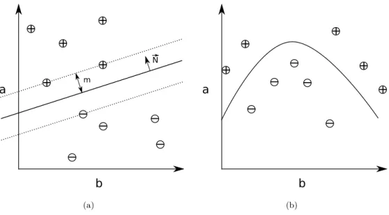
The Support Vector Machine is a machine learning method that constructs a hyper-dimensional plane to separate instance vectors of different classes. This hyperplane is constructed to have maximal margin to in-stance vectors of each class. The vectors closest to the dividing hyperplane are called the support vectors, and

(13)

a

b

+

-+

-m N (a)

a

b

+

-+

+

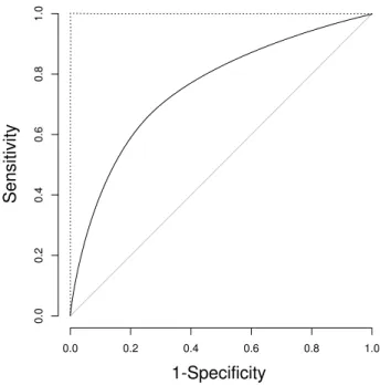
(b)

Figure 3.1: 3.1(a): Example of a 2-dimensional feature space with instances drawn as⊕and corresponding to positive and negative classes, respectively. The hard line is a potential dividing line, and the dotted lines denote the margins. N~ denotes the normal of the dividing line. 3.1(b) Example of a case where a line is unable to properly separate the training instances, but a non-linear surface can separate them.

the support vectors define the hyperplane with maximal margin. For a soft-margin classifier, some instance vectors may be ignored (treating them as noise), which may give better generalization than its alternative, called a hard-margin classifier [21]. Figure 3.1(a) illustrates this in two dimensions.

Definition 10 (Dot product) ~a·~b=Pq

i=1ai∗bi for~a,~b∈Rq denotes the dot product of vectors~aand~b.

To construct a linear classifier, a hyperplane can be constructed to optimally separate the training in-stance vectors. Such a hyperplane can be represented by the vector equation N~ ·~x = b, where N~ is the hyperplane normal vector,~xis an arbitrary vector andb is an offset term. The signed distance from some instance vector ~xto this hyperplane isN~ ·~x−b, where the sign may be used to assign a discrete class,i.e. ˆ

c(~x) =sgn(N~ ·~x−b) [21].

It may be that the instance vectors are distributed such that there is no hyperplane that separates the instance vectors. Figure 3.1(b) illustrates this issue. A non-linear classifier can be constructed by applying the kernel trick. This will be discussed in the next section.

3.3

Kernel function

The kernel trick involves using a transformation Φ(~x) = x~∗ _{that maps vectors} _~_x _∈

Ra to vectors in a

higher-dimensional space x~∗ _∈

Rb, b > a. Based on this transformation, one can define the kernel function

k(~x, ~y) = Φ(~x)·Φ(~y), which evaluates the dot product in this higher-dimensional space in terms of vectors in the original space. A linear classifier may then be constructed to separate vectors in this higher-dimensional space [21]. The decision function then may be ˆc(~x) =sgn(N~ ·Φ(~x)−b).

The kernel function has a particular utility in the context of Support Vector Machines. The decision function of a Support Vector Machine makes use of the fact that the normal of the dividing hyperplane can be expressed in terms of the support vectors:

~ N = l X i=1 αiyiΦ(x~i).

(14)

Here, l is the number of training instance vectors,x~i are training instance vectors, yi are the associated

target values (such as 1 for a positive instance and −1 for a negative instance), and αi are Lagrangian

multipliers, where for support vectorsαi>0 [21]. Substituting this into the decision function gives:

ˆ c(~x) =sgn l X i=1 αiyiΦ(x~i)·Φ(~x)−b ! . But this means that:

ˆ c(~x) =sgn l X i=1 αiyik(x~i, ~x)−b ! .

Thus, the decision function is formulated in terms of the kernel function, which can be simplified in terms of vectors in the original space. Thus, the computational complexity is not significantly increased by this mapping to higher-dimensional space.

In this thesis, the Support Vector Machine implementation in LibSVM will be used. Kernel functions provided in LibSVM include [23]:

• the linear kernel: k(~x, ~y) =~x·~y;

• the polynomial kernel: k(~x, ~y) = (γ~x·~y+c0)d, γ >0; • the radial basis function kernel: k(~x, ~y) =e−γk~x−~yk2

.

For these kernels, the parameters γ, c0 andd are called kernel parameters. When used in this thesis,d

will be locked to 2 and 3, referred to as quadratic and cubic kernels, respectively.

3.4

SVM formulations

There are multiple Support Vector Machine formulations. The formulations dictate how the Support Vector Machine is constructed from the training vectors. The formulations in LibSVM areC-Support Vector Classi-fication,ν-Support Vector Classification, one-class SVM,-Support Vector Regression andν-Support Vector Regression [24].

TheC-Support Vector Classification requires only a parameter C >0 [24], which is called the cost pa-rameter, as an increase in C corresponds to treating errors as being more expensive when constructing the SVM [21]. Additionally, it supports the use of multiple classes. To use C-Support Vector Classification, class membership probabilities can be obtained for each class. Classification with more than two classes can be made binary by combining the probabilities into a score. In this thesis, the maximum probability for belonging to a positive class will be multiplied by one minus the maximum probability for belonging to a negative class to make a score. Additionally, the C-Support Vector Classification supports the weighting of different classes, which may be useful when when the training data is unbalanced [24].

Theν-Support Vector Classification only requires a parameterν ∈(0,1], which controls for the fraction of training errors versus fraction of support vectors [24].

The one-class SVM formulation requires the parameter ν ∈ (0,1] [24]. An interesting property of the one-class SVM is that only training instances of one class, the positives, are used during construction. By the standard implementation in LibSVM, one-class SVM does not give a continuous classification value. How-ever, it can be tricked by switching its type to -Support Vector Regression after training, as it is handled identically in most cases after training.

Additionally, Support Vector Regression can be used to approximate a real valued function. The-Support Vector Regression has the cost parameterC >0 in addition to a parameter >0 [24]. Theν-Support Vector

(15)

Regression has both the cost parameter C >0 andν∈(0,1] [24].

The C-Support Vector Classification only requires the C parameter. The selection of parameters, dis-cussed later, is automated and requires up to many training cycles, so a reduced number of parameters is useful. At the same time, the LibSVM implementation of the C-Support Vector Classification formulation clips probabilities as they approach 1, and this can pose issues when a larger threshold is desired (for example due to wanting very few predictions expected by chance). The -Support Vector Regression implementation on the other hand does not clip output values.

(16)

Chapter 4. Classifier validation 11

Chapter 4

Classifier validation

When one has constructed a classifier, one needs a way to measure how well it performs. This could for example be in order to compare different algorithms applied to the same kind of classification problem, or to compare multiple runs of the same algorithm but with different parameters. One may wish to determine how well an algorithm approximates the training data, and how well one might expect it to generalize to unobserved instances of the domain under investigation.

4.1

The confusion matrix and associated statistics

If the classification problem is binary, the classifier may return a score for an objectx∈X, such that a larger value indicates larger confidence thatxbelongs to the class one is trying to predict members of.

Definition 11 (Binary label set) B={⊕, } is the set of positive and negative classification labels,

re-spectively.

Definition 12 (Binary label assignment function) For a real valuey∈R,[y]± ∈Bdenotes a function assigning a binary class label for y, such that[y]_± =⊕if y >0, and[y]_± = otherwise.

If the classifier is of the form ˆc(~x)≈c(~x) =y, where~x∈Rd is an instance vector and y∈R denotes a

score, one obtains a binary classification for the classifier by applying a score threshold as [ˆc(~x)−t]_±. Given a set of pairs of instance vector and unique labelsS ⊂Rd×B, the following sets can be defined:

Definition 13 (Original set classes)

P(S) ={~x|(~x, y)∈S, y=⊕}

N(S) ={~x|(~x, y)∈S, y= }

whereP(S)∩N(S) =∅

Definition 14 (Predicted set classes)

ˆ P(S,ˆc, t) =~x|(~x, y)∈S,[ˆc(~x)−t]_±=⊕ ˆ N(S,ˆc, t) = ~ x|(~x, y)∈S,[ˆc(~x)−t]_±= ˆ P(S,ˆc, t)∩N(S,ˆ ˆc, t) =∅

These constitute the sets of instance vectors that are positives, the ones that are negatives, the ones that are predicted as positives and the ones that are predicted as negatives, respectively. The condition P(S)∩N(S) = ˆP(S,c, t)ˆ ∩Nˆ(S,ˆc, t) =∅ensures that only one label is assigned to each instance vector. Also, positives and negatives together cover all instance vectors of S, soP(S)∪N(S) = ˆP(S,ˆc, t)∪N(S,ˆ ˆc, t).

The relationship between predicted classes and actual classes may be summarized in a table called the confusion matrix. This will here be defined for the binary case.

(17)

Definition 15 (Set cardinality) For a setS,|S|refers to its cardinality, its number of elements.

Definition 16 (Confusion matrix values) The measures True Positives, True Negatives, False Positives and False Negatives, respectively, are defined as follows.

T P(S,ˆc, t) =|P(S)∩Pˆ(S,ˆc, t)|

T N(S,ˆc, t) =|N(S)∩Nˆ(S,ˆc, t)|

F P(S,c, t) =ˆ |N(S)∩P(S,ˆ ˆc, t)|

F N(S,c, t) =ˆ |P(S)∩_N(S,ˆ _ˆ_{c, t)}_|

For simplicity, the parameters ofT P,T N, F P andF N will be dropped when they are not informative.

Definition 17 (Confusion matrix) The confusion matrix for a binary classification problem is a 2x2 con-tingency table indicating the agreement and disagreement between predicted classes and actual classes [25].

ˆ P Nˆ P T P F N N F P T N

A first measure that may be defined from the confusion matrix is the fraction of positives that are pre-dicted as positives, known as the Sensitivity,True Positive Rate (TPR) and Recall [26]. In this thesis, the wordSensitivity will primarily be used.

Definition 18 (Sensitivity)

Sensitivity=T P R=Recall= T P T P +F N

Similarly, a useful measure that can be defined from the confusion matrix is the fraction of predicted positives that are actual positives, known as thePositive Predictive Value (PPV) andPrecision [26]. When used together withSensitivity, the namesRecallandP recisionwill be used.

Definition 19 (Positive Predictive Value)

P P V =P recision= T P T P +F P

It is also useful to measure how many of the negatives are predicted as positives, known as the False Positive Rate (FPR) [26]. There is also the equivalenceF P R= 1−Specif icity. When used together with T P R, the namesSensitivity and 1−Specif icity will primarily be used, or otherwiseT P RandF P R.

Definition 20 (False Positive Rate)

F P R= 1−Specif icity= F P F P+T N

One way to measure the overall classifier performance from the confusion matrix is to measure the pro-portion of instances that are correctly classified, which is referred to as theAccuracy [24].

Definition 21 (Accuracy)

Accuracy= T P +T N T P +F P+T N+F N

An issue with this measure is that if the set of positives is larger than the set of negatives, thenT N will have less of an impact on the Accuracy than T P. Similarly, if the set of negatives is larger than the set of positives, then T N will have a larger impact than T P. An alternative measure that uses all four of the confusion matrix values is Matthews Correlation Coefficient (MCC) [25].

(18)

Definition 22 (Matthews Correlation Coefficient)

M CC= _p T P ∗T N−F P ∗F N

(T P+F P)(T P +F N)(T N+F P)(T N+F N)

Sometimes, T N may be unknown or not well-defined. In such cases, an alternative to Accuracy and M CC is theF-measure, which combinesP recisionandRecall, and thus does not useT N [27].

Definition 23 (F-measure)

Fβ = (1 +β2)

P recision∗Recall (β2_∗_{P recision) +}_Recall

β >0 is a weighting ofP recisionversusRecall. Forβ >1,Recall has a larger impact on the fraction than P recision, and opposite for 0< β <1.

4.2

Continuous quality measures

The confusion matrix values are discrete, in the sense thatT P,T N F P and F N directly depend upon the size of the labelled set used for evaluation. Thus, the measures based on the confusion matrix values are also discrete. In certain cases, it can be useful to have continuous quality measures. For the binary case, continuous classification scores can be used. To define quality measures based on such values and allow the same values to occur multiple times, the values can be collected in vectors. One measure is the Pearson correlation coefficient [25].

Definition 24 (Pearson Correlation Coefficient) For a vector S= [s1, ..., sn]∈Rn, let S = 1n Pn

i=1si

denote the mean vector component. Similarly, letσS denote the standard deviation of components ofS. For

vectorsA, B∈Rn, whereA= [a1, ..., an]andB = [b1, ..., bn], the Pearson Correlation Coefficient is given by

C(A, B) = n X i=1 (ai−A)(bi−B) σAσB .

Definition 25 (Pearson Correlation Coefficient for classification values) Consider a setV ={(~x1, y1), ...,(~xn, yn)}

of n validation elements with labels yi ∈ B. Let f(yi) = 1 if yi = ⊕and f(yi) = −1 if yi = . A vector

of classification values can be denoted as c = [ˆc(x~1), ...,ˆc(x~n)]. Similarly, a vector of target values can be

denoted as v= [f(y1), ..., f(yn)]. The Pearson Correlation Coefficient between candv can then be used as a

quality measure.

For a classifier ˆc, this quality measure gives the correlation coefficient between the classification values ˆ

c(~xi) and values based on correct labels for each~xi (1 for a positive label and−1 for a negative label). The

respective means are subtracted from classification and target values, and the measure is scaled down by the standard deviations. Accordingly, the measure is determined by the distance of each classification values to the classification mean, with values closer to the mean having a smaller impact. When the target value and classification value are one the same side of their respective means, the measure increases, and otherwise it decreases.

The sum of squared errors has been used in gradient descent for measuring the error during training of neural networks [22]. A quality measure can be made by using one minus the sum of squared errors.

Definition 26 (1-sum of squared errors) Consider a set V ={(~x1, y1), ...,(~xn, yn)} of nvalidation

ele-ments. Let f(b) = 1if b =⊕ andf(b) =−1 if b= . A vector of classification values can be denoted as c= [ˆc(x~1), ...,ˆc(x~n)]. Similarly, a vector of target values can be denoted asv= [f(y1), ..., f(yn)].

1−E2= 1− n X

i=1

(19)

Chapter 4. Classifier validation 14 0.0 0.2 0.4 0.6 0.8 1.0 0.0 0.2 0.4 0.6 0.8 1.0 1-Specificity S ensi tivi ty

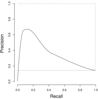
Figure 4.1: Example of a Receiver Operating Characteristic curve (solid line). The dotted line corresponds to a perfect classification. The diagonal corresponds to random classification.

4.3

Receiver Operating Characteristic curves

For binary classification as defined above, [ˆc(~x)−t]_±, the measuresT P, T N, F P andF N are functions of the threshold valuet. Whentis maximal, all classifications will be negative. Astis decreased, more instances are classified as positive, until all instances are classified as positive. Thus, measures using confusion matrix cells may be plotted against one another by varying the thresholdt.

Definition 27 (Receiver Operating Characteristic curve) Receiver Operating Characteristic curves (ROC curves) are plots of the Sensitivity in the y-axis against1−Specif icityin the x-axis [5].

An example of a ROC curve is shown in Figure 4.1. Starting with no positive classifications gives a point in the bottom left of the plot, and as t is decreased and the classifier gives more positive classifications, some may be correct (contributing to theSensitivity, upward) and some may be incorrect (contributing to 1−Specif icity, rightward). Thus, a good classifier will have a ROC curve tending towards the upper left of the plot. A random classification will be around the diagonal. The construction of a Receiver Operating Characteristic curve is illustrated by Algorithm 3. This procedure could be optimized by ordering classifier score and label pairs according to scores and iteratively updating the confusion matrix values.

Since the ROC curve of a good classifier will tend towards the upper left of the plot, a quality measure has been defined to capture this tendency, called the Area Under the Curve (AU C or AU ROC) [28]. This measure calculates the area under the ROC curve. In some cases, it may be desirable to only capture the classifier performance for lower 1−Specif icity, and thus this measure will be defined as a function of thex axis coverage.

Definition 28 (ROC Area Under the Curve (AU C)) Based on a ROC curve, the area under the curve in the interval0≤1−Specif icity≤xcan be calculated, and this will be referred to as AU C(x).

The regularAU C/AU ROCis then given byAU C(1). This measure can be calculated by gradually gener-ating points on the ROC curve and summing up areas below the curve. Algorithm 2 demonstrates the method.

(20)

Algorithm 1ROC plot construction

Input:

C∈R×B: A set of paired classifier scores and correct labels.

makeP oint(x, y): Makes a plot point with X-positionxand Y-position y. makeLine(a, b): Makes a line from pointato pointb.

S← {v|(v, f)∈C} ∪ {−∞} . Get scores from the classifications for thresholds. . For the final iteration, all should be classified as positive, thus the added−∞. pa←0

while S6=∅do

t←maxS . Get maximum scoring classification, to be used as a threshold.

S←S/t . Remove it from the list.

T P, F P, T N, F N←0

for all(v, f)∈C do . Find confusion matrix values for the cutoff.

if v > tthen if f =⊕then T P ←T P+ 1 else F P ←F P+ 1 end if else if f =⊕then F N←F N+ 1 else T N ←T N+ 1 end if end if end for T P R← T P T P+F N F P R← F P F P+T N

pb←makeP oint(F P R, T P R) . Note the point as the current line end ...

if pa6= 0then

makeLine(pa, pb) . ... and make a line if there is a line start.

end if

pa ←pb . Make this line end be the start of the next line.

(21)

Algorithm 2Calculation of theAU C(x) measure

Input:

functionAU C(x)

S← {v|(v, f)∈C} ∪ {−∞} . Get scores from the classifications for thresholds. . For the final iteration, all should be classified as positive, thus the added−∞. AU C←0

F P Ra ←0

T P Ra ←0

whileS6=∅do

T P, F P, T N, F N ←0

if v > tthen if f =⊕then T P ←T P + 1 else F P ←F P + 1 end if else if f =⊕then F N ←F N+ 1 else T N ←T N+ 1 end if end if end for

T P Rb← T PT P+F N . Get new ROC point.

F P Rb← F P+T NF P if F P Rb > xthen . Restrict to 0≤F P Rb≤x. F P Rb←x T P Rb←T P Ra+ (x−F P Ra)(T P Rb−T P Ra) end if a←F P Rb−F P Ra AU C←AU C+aT P Ra+a₂(T P Rb−T P Ra)

if F P Rb =xthen . End at the desired False Positive Rate.

break end if T P Ra←T P Rb F P Ra←F P Rb end while returnAU C end function

(22)

Chapter 4. Classifier validation 17 0.0 0.2 0.4 0.6 0.8 1.0 0.0 0.2 0.4 0.6 0.8 1.0 Recall P re cisi on

Figure 4.2: Example of a Precision/Recall curve. The dotted line marks a perfect classifier. The grey line marks random classification performance.

4.4

Precision/Recall curves

In some cases, the set of True Negatives,T N, may not be well-defined. For example, if the classification task is to mark certain phrases in a document, thenT N is the set of regions marked neither in the validation set nor by the classifier, and is thus not well-defined defined due to the number of phrases in a document not being well-defined [27]. T N could also be very large, such that the curve could tend towards the upper left even if there are many false positives for each true positive. P recision andRecall do not depend on T N, and this gives an alternative plot for visualizing classifier performance.

Definition 29 (Precision/Recall curve) In a Precision/Recall plot (PR plot), P recision is plotted on the y-axis andRecall on the x-axis [26].

An example is shown in Figure 4.2. Similarly to the construction of ROC plots, PR plots are constructed by varying the thresholdt. The construction of a Precision/Recall curve is illustrated by Algorithm 3. The approach is mostly identical to the construction of a ROC plot, except for usingP recisionandRecall.

For interpreting PR plots, it can be noted that going from left to right in a PR plot corresponds to increasingSensitivity. The higher a point on the curve is, the higher the portion of positive classifications are correct. Thus, an ideal curve would cover the top of the plot. It has also been shown that a classifier dominates in a ROC plot if and only if it dominates in a corresponding PR plot [26]. A random classifier will have performance around a line flat overRecall, whereP recision= _|_P|_|₊P|_|_N_| [29]. However, calculating the expected random performance by this definition requires knowing N, and thusT N, and as noted these may be unknown.

4.5

Measuring generalization

A trained classifier can be applied to classify the training data to see how well it has been learned. However, it is usually more useful to measure how well one might expect the classifier to classify instances of the larger

(23)

Algorithm 3PR plot construction

Input:

makeP oint(x, y): Makes a plot point with X-positionxand Y-position y. makeLine(a, b): Makes a line from pointato pointb.

S← {v|(v, f)∈C} ∪ {−∞} . Get scores from the classifications for thresholds. . For the final iteration, all should be classified as positive, thus the added−∞. pa←0

while S6=∅do

T P, F P, T N, F N←0

if v > tthen if f =⊕then T P ←T P+ 1 else F P ←F P+ 1 end if else if f =⊕then F N←F N+ 1 else T N ←T N+ 1 end if end if end for P recision← T P T P+F P Recall← T P T P+F N

pb←makeP oint(P recision, Recall) . Note the point as the current line end ...

if pa6= 0then

makeLine(pa, pb) . ... and make a line if there is a line start.

end if

pa ←pb . Make this line end be the start of the next line.

(24)

class under investigation. One approach to this is to apply the classifier to a set separate from the training data. This may not be practical if only a few instances of the class are known, as it may be desirable to use all of these instances for training. The technique of cross-validation provides an alternative.

The basic idea of cross-validation is to train the classifier on a subset of the training set and classify the remainder [21]. As the classified elements have not been used during training, this gives a measure of generalization. A confusion matrix can be constructed based on the resulting classifications.

Definition 30 (n-fold unbalanced cross-validation) For a training setT ⊂X×C, shuffle its elements randomly and divide it inton (approximately) evenly sized subsets T1, ..., Tn (folds). For each foldi∈[1, n],

train the classifier on T1∪...∪Ti−1∪Ti+1∪...∪Tn, and use the trained classifier to classify Ti [21].

The unbalanced cross-validation approach derives its name from the fact that it does not consider the number of training examples for each class. If there are many more training examples of one class than of others, this could in some cases lead to folds with few or no training examples for some class or classes. An alternative is to first partition the training set according to classes, divide these partitions into class-specific folds, and join class-specific folds to form the folds used.

Definition 31 (n-fold balanced cross-validation) For a training setT ⊂X×Cwithmclasses, divideT into subsetsT1, ..., Tmaccording to class. For each classj ∈[1, m], shuffle the corresponding subset randomly, and divide it inton(approximately) evenly sized subsetsT₁j, ..., Tj

n(folds). For each foldi∈[1, n], make joined

subsets Ti=Ti1∪...∪Tim. For each foldi∈[1, n], train the classifier onT1∪...∪Ti−1∪Ti+1∪...∪Tn, and

use the trained classifier to classify Ti.

The number of folds can be selected to control for how many times the classifier is trained. Both balanced and unbalanced cross-validation use randomization for constructing the folds. Thus, there may be noise in quality measurements made on the folds. To reduce this issue, n-fold cross-validation can be repeated k times, and the quality can be measured over the full set of classifications, or it can be measured for each repeat and averaged. Alternatively, cross-validation can be done by only leaving a single training example out during training for validation, called Leave-One-Out cross-validation.

Definition 32 (Leave-One-Out cross-validation) For a training set T ⊂ X ×C, let its elements be denoted by t1, ..., tn. For each element ti ∈ T, train the classifier on {t1, ...ti−1, ti+1, ..., tn} and use the

(25)

Chapter 5. Prediction of Polycomb/Trithorax Response Elements with Support Vector Machines 20

Chapter 5

Prediction of Polycomb/Trithorax

Response Elements with Support

Vector Machines

In this thesis, Support Vector Machines are applied to the prediction of Polycomb/Trithorax Response Elements. This carries with it a series of design choices. The ideal is to develop an application that can take example sequences and additional parameters, and predict PREs in a given genome without further user intervention. The implementation of Polycomb/Trithorax Response Element prediction in this thesis is named PRESVM (read pre-S.V.M.). First, the use of Support Vector Machines for PRE prediction will be discussed, and then the design of PRESVM will be explained.

5.1

Why Support Vector Machines may improve prediction of

PREs

The PREdictor scores sequence windows by summing weighted frequencies of paired motif occurrences within 220bp. Applying the PREdictor genome-wide with a score threshold calibrated for anE-value of 1, Ringrose et al. were able to identify 167 candidate Polycomb/Trithorax Response elements [1]. Since paired motif occurrences were found to be predictive of PREs, this may indicate non-linear relationships between motif occurrence frequencies.

Support Vector Machines have properties that could be beneficial for the prediction of Polycomb/Trithorax Response Elements. Any real valued features may be used with Support Vector Machines, so there may be feature sets other than paired motif occurrence frequencies that could help the prediction task. There might also be non-linear relationships between feature values, which an SVM might model.

In early 2012, Zeng et al. [2] published a Support Vector Machine implementation of PRE prediction. They found that non-linear kernels better distinguished PREs from non-PREs than a linear kernel. Thus, PRESVM is not the first Support Vector Machine implementation of PRE prediction. However, Zeng et al. [2] used single motif occurrence frequencies in windows as features for the SVM, so the question remains of whether other real valued feature sets might give improved PRE prediction. There are also additional considerations, such as selecting parameters for the Support Vector Machine and how to construct training vectors from training sequences.

(26)

Parameter input

Feature selection

Parameter optimization

Validation

Cutoﬀ calibration

Validation

Proﬁle generation

Genome-wide prediction

Figure 5.1: The PRESVM pipeline. A dotted box indicates that the step is optional.

5.2

PRESVM

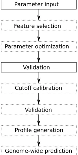
PRESVM has been designed such that it after being supplied with parameters runs through all steps needed to make genome-wide predictions of PREs without requiring further user intervention. It is also useful to be able to evaluate different configurations without making genome-wide predictions. Thus, PRESVM consists of a pipeline with a series of optional steps, depicted in Figure 5.1.

The compulsory parameters are: 1) at least one feature set, 2) a set of motifs and 3) training sequences. Additional pipeline steps that should be executed can be specified. With threshold calibration and/or genome-wide prediction, a genome must also be specified.

In the feature selection step, a subset of the specified features are selected using mRMR feature selection [30]. In the parameter optimization step, a search is run for optimal SVM parameters. In the validation step, a classifier is constructed with the given configuration and is applied to the training sequences for vali-dation, as well as any specified sets of validation sequences. During the cutoff calibration step, the classifier is applied to a large, randomly generated sequence, such that a cutoff is chosen for a desiredE-value. After the cutoff calibration step there is a second validation step, such that the influence of the resulting cutoff on classification performance may be investigated. A profile is then generated to describe the run. Finally, the classifier is applied genome-wide for prediction. These steps are described in more detail later.

(27)

The profile generation step outputs a profile in XML format. This profile contains a detailed description of the configuration that was used during the run, as well as paths to files generated during genome-wide prediction. It also contains validation sequence scores, which can later be used for visualizing classifier per-formance via ROC and PR curves.

5.3

Support Vector Machines and sequences

To apply Support Vector Machines to the prediction of PREs, it must be decided how the classifier should be trained and how it should be applied for prediction. First, sequences and sequence coordinates can be defined.

Definition 33 (Sequence) A sequenceS ∈Snt is a string of nucleotides (A,T,G andC).

Definition 34 (Sequence coordinates) For a sequence S ∈_S_nt andA, B ∈_N where A ≤ B, S : A...B denotes the subsequence ofS from nucleotideA (base1) up to and including nucleotide B.

Definition 35 (Sequence length) For a sequenceS :A...B,S∈Snt,λ(s) =B−A+ 1denotes its length.

The goal is to train a classifier and apply it across a whole genome to predict PREs. As was done with the PREdictor [1], the classifier can be applied across the genome using a sliding window.

Definition 36 (Sequence sliding window) For a sequenceS:A...B,S∈Snt, a sliding window will refer

to a function

W(S, w, s, i) =S:X...Y

where X = A+s(i−1) and Y = min{X+w−1, B}. w >0 is the window width, s > 0 is the window stepping and i is the window index (base1). When no range is specified,i goes from1 up to including only one window whereY =B.

Assume there are training sequencesS1, ...Snand featuresf1(Si), ..., fm(Si). The features can be applied

to the full training sequences for constructing training vectors, or they can be applied using a sliding win-dow over the sequences, giving a training vector for each winwin-dow. Using a sliding winwin-dow to make training vectors may give a very large training set, but a larger step size can be used during training to make up for this. Alternatively, one or more windows may be selected from each sequence as representative to construct training vectors.

It has been suggested that it is important that the feature values are scaled and shifted to have the same range over the training examples, and the same scaling and shifting should also be used when the trained classifier is to be applied for classification [23].

In the case of non-PRE sequences, it can be noted that every window in a non-PRE training sequence should correspond to a negative, and thus either the full sequences or sequence windows can be used for constructing training vectors.

In the case of PRE sequences, it may be that up to many of the sequence windows are not important for PRE function. The PREdictor [1] PRE training sequences have lengths in the range 1.2kb−5.4kb, whereas it has been suggested that PREs have lengths of only a few hundred base pairs [6]. Also, the sequences may vary in length, as with the PREdictor [1] training sequences, which has implications both for training with the full sequences and with sequence windows. If the full sequences are used for training, there are certain feature sets (discussed in Chapter 6) where sequence lengths are used for normalization, and because of this, differing sequence lengths might result in important features being normalized away. If training is done using sequence windows, there may be more windows for some sequences. For using sequence windows for training, it should be noted that a soft-margin classifier might treat irrelevant windows as noise. If irrelevant windows put constraints on the decision surface and thus distort it, then the exclusion of these windows could lead to a decision surface that better separates PREs from non-PREs. Alternatively, representative sequence windows

(28)

might be selected directly. However, for trying to select representative windows directly from the training sequences, it may be difficult to decide on a good selection criterion, and a poor selection criterion might have a negative impact on the resulting classifier.

After a classifier has been trained, it is desirable to apply it to sequences for validation, such as the training sequences. Since the classifier will be applied across the genome using a sliding window, it makes sense to also apply it using a sliding window during validation. If all validation sequence window scores are used to measure classification performance, there is the potential issue that longer sequences may have more windows, and thus have a higher influence on the classification performance measurement. To avoid this, the window scores for each validation sequence can be combined into a single sequence score. In this thesis, this will be done by letting the maximum window score for a sequence be the score of the full sequence, as was done with the PREdictor [1].

score(S) = max

i c((fˆ 1(W(S, w, s, i)), ..., fm(W(S, w, s, i))))

The classifier threshold may then be applied to obtain a binary classification for each sequence, and this enables the construction of a confusion matrix for the validation sequences.

5.4

Training data

To train a classifier to predict PREs genome-wide, it is necessary to have a set of known PRE sequences for the classifier to learn from. For Support Vector Machines, other than in the case of one-class SVM, it is also necessary to have sequences of one or more non-PRE classes to learn from. In this thesis, the training data used by Ringrose et al. [1] will be used. Additionally, the construction of alternative training data will be explored briefly.

After a classifier has been trained, one may attempt to apply the trained classifier to the PRE training sequences in order to identify significant sub-sequences. If the classifier can already be expected to give reasonable genome-wide predictions of PREs, it may be hoped that the classifier will assign higher scores to the more important PRE training sequence regions. One may then apply the trained classifier to the PRE training sequences and select an equal number of high-scoring windows from each training sequence as representative. These windows can then be used to train a new classifier. This is referred to as re-training in this thesis. If the selected windows are indeed important for PRE function, the removal of other sequence regions might amplify relevant features, and thus might improve prediction.

Ringroseet al. [1] defined PREs based on published coordinates of known PRE/TREs. For non-PREs, they used promoter regions of genes that are regulated by the Z and GAF motifs. When using a multi-class SVM, it is possible that training with additional classes may have an impact on predictions. One may for example add a class of randomly generated sequences with the same nucleotide distribution as the genome, corresponding to non-PREs.

In addition to the training sequences used by Ringroseet al. [1], it may be interesting to train a classi-fier using data from the recent genome-wide ChIP-chip/ChIP-seq studies, such as [12, 14, 15]. For positive (PRE) training examples, experimentally determined regions can be selected. If a selection of sequence mo-tifs have already been chosen to be used for the classification task, the regions may be filtered for having occurrences of these motifs. Alternatively, motifs can be selected based on the experimentally determined regions. The selected regions can further be filtered, for example according to whether or not they are in-tergenic. Afterwards, a selection of the regions can be selected randomly and taken as PRE training examples. For negative training examples, one would ideally want to select genomic regions that one can be fairly confident are not PREs. If sequence motifs are used, one possibility is to find genomic regions that are enriched in the sequence motifs and randomly select a number of regions and use them as non-PRE training examples. As the regions are selected due to being enriched in the motifs, but paired occurrences of motifs

(29)

are more predictive of PREs [1], it may be speculated that perhaps many or most of the selected regions will not be PREs. However, there is a risk of selecting PREs using this approach. With a soft-margin classifier, it is possible that false negatives will be filtered out as noise.

An alternative to selecting a set of non-PRE training examples is to use Mapping-Convergence, as was re-cently done for the prediction of PcG target genes in humans using Support Vector Machines [20]. Mapping-Convergence starts with a positive set and an unlabeled set, and the unlabeled set is used to iteratively construct a negative training set. This has not been implemented in PRESVM.

5.5

Genome-wide prediction

When predicting PREs in a genome, the classifier is applied across a whole genome in windows. Each window will be given a score by the classifier, and this results in a score profile for each chromosome. In PRESVM, these score profiles are exported to a Wiggle format file. This format was chosen due to its support by the Integrated Genome Browser [31], and is explained in UCSC Genome Bioinformatics FAQ for formats [32]. The Wiggle format is a human readable format, containing chromosome names, window coordinates and corresponding profile values. The Wiggle format allows defining the length and step size for windows at the start of a chromosome, such that the window scores may be given compactly, separated by line breaks. In addition to being able to visualize such score profiles using the Integrated Genome Browser, such score profiles also allow for other informative analyses, such as the correlations between different profiles. A score threshold is applied to give binary classifications to windows. When applying a threshold to window scores, overlapping positively classified windows are merged, giving a selection of non-overlapping predicted regions in the genome. Such regions will here be referred to asbands.

Definition 37 (Band) Bands will refer to positively classified regions, where overlapping regions have been merged.

In PRESVM, predicted bands are exported to a General Feature Format (GFF) file, and as with the Wiggle format it was chosen due to its support by the Integrated Genome Browser [31], and is explained in UCSC Genome Bioinformatics FAQ for formats [32]. GFF is a human readable format. GFF files consist of lines specifying genomic regions. In addition to visualizing GFF files with the Integrated Genome Browser, these files are also useful for investigating the overlap of predictions with experimentally determined regions and what annotated genes are proximal to each predicted band. Genome-wide prediction is illustrated by Algorithm 4.

5.6

Classifier threshold calibration

To predict genomic regions as being PREs, the classifier threshold must be set to a reasonable value. It is desirable to set the threshold such that one has an idea of how many positive predictions can be expected by chance. That is, it is desirable to select the threshold for some desired E-value. In this thesis, this will be done similarly to how it was done with the PREdictor [1].

First, the distribution of nucleotides in the genome is found. Based on this distribution, a random se-quence is generated. A trained classifier ˆcis applied to this sequence in windows as it would for genome-wide prediction. If this sequence is of the same length as the genome, then the number of predictions made on this randomly generated sequence for some thresholdt gives an approximate E-value. Thus, the threshold can be varied, and the approximate E-value can be noted for each threshold. This gives an approximated E-value distribution. The final threshold can then be selected based on theE-value one desires.

(30)

Algorithm 4Genome-wide prediction

Input:

Chromosomes: Set of chromosome sequences. ˆ

c:_Rn_→

R: Classifier.

f1, ..., fn :Snt→R: Sequence features.

wsize∈N: Window width (w≥1).

wstep∈N: Window step size (s≤w).

P ← ∅ . Set of genome-wide predictions.

for allC:A...B∈Chromosomesdo

i←A

pa, pb← −1 . This will note the start/end of a prediction when not−1.

loop

j←min{i+wsize, B}

W ←C:i...j . Get the window, cropped by the sequence length.

v←ˆc((f1(W), ..., fn(W))) . Score the window.

if v > tthen . Score above threshold so update prediction.

if pa=−1 then

pa ←i . Prediction not started, so note start.

end if

pb←j

else if pa6=−1∧i > pb then . Score below cutoff, and passed prediction end, so finish it.

P ←P∪ {C:pa...pb} . Register prediction.

pa, pb ← −1

end if

i←i+wstep

if j=B then . Last window in the sequence, so break out of the reading loop.

break end if end loop

if pa6=−1then . Finish any open prediction.

P ←P∪ {C:pa...pb}

end if end for returnP

(31)

If the desiredE-value is low, such as 1, the threshold found can be expected to vary significantly from run to run when the randomly generated sequence is of the same length as the genome. The threshold can be made more stable by scaling up the size of the randomly generated sequence, and scaling down the approximatedE-values. Letb(ˆc, t) denote the number of predictions made by a classifier ˆcon the randomly generated sequence when using thresholdt. Letldenote the size of the genome, lets≥1 be a scaling factor, and let the length of the randomly generated sequence bel∗s. The approximatedE-value is then given by:

ˆ

Ebands(ˆc, t) =

b(ˆc, t) s ,

The scaling factor s can be used to make the thresholds for E-values more stable. Given a constant probability for each window in the randomly generated sequence to be predicted, increasing the length of the sequence increases the expected number of predicted windows, and thus the number of predicted bands is divided by the scaling factor. This in turn reduces the influence of individual predictions on the approximated E-value.

It then needs to be decided how the threshold should be varied. One could find all window classification values over the full randomly generated sequence, and then iteratively use each as a threshold and find the number of predictions (bands) in the random sequence. This can be computationally very expensive if the scaling is large. Typically, a lowE-value, such as ˆEbands(ˆc, t) = 1 is desired. To make the threshold fairly

stable a large scaling factor such as s = 100 should be used. Thus, it is desirable to have a more efficient approach for varying the threshold.

If theE-value of interest is low, there should be a limited amount of predictions in the randomly generated sequence. Each of these predictions may be based on up to multiple overlapping window classifications, but the number of overlapping positively predicted windows should then typically be limited. A possibility then is to findntop-scoring windows in the randomly generated sequence. The threshold can then be varied over the scores of these windows. As these windows are top-scoring, only these windows would be classified as positive in the randomly generated sequence when using their scores as threshold values, and one can therefore avoid classifying all windows from the randomly generated sequence multiple times. For each threshold, taking the overlaps between positively predicted top-scoring windows into account gives the predicted regions, and this can be used to get a corresponding approximated E-value.

This approach, called the highscore based E-value threshold calibration method, is implemented in PRESVM. An issue with this approach is that the number n of top-scoring windows to find in the ran-domly generated sequence must be decided. If n is too small, the threshold for the desired E-value may not be found. One possibility is to select nbased on an expectation of how many windows will overlap in a prediction. If one expectsioverlapping windows for a prediction, one possibility is to usen=i∗s∗E, where E is the desiredE-value andsis the scaling factor for the randomly generated sequence. In PRESVM, nis chosen by the following equation

n= 2s∗E∗ wsize

wstep

where wsize is the window size used andwstep is the sliding window step size. Thus, if the step size is

de-creased,nwill increase. This makes sense, since if the step size is reduced, one would expect more overlapping windows to be predicted as positive. The chosennmay be larger than necessary, but this should reduce the probability of nbeing too small. The approach is illustrated in Algorithm 5.

Another way to vary the threshold is to find the range of window classification values over the genome, and to divide this range into m evenly spaced thresholds. The classifier is then applied to the randomly generated sequence, and the number of predictions for each threshold is noted. The approximated E-value for each threshold is then calculated based on the corresponding number of predictions.

As shown for genome-wide prediction, predictions can be made as the classifier is applied to the sequence. Thus, this approach can be implemented by keeping the necessary prediction state variables for each of the

(32)

Algorithm 5Highscore basedE-value threshold calibration

Input:

ˆ c:_Rn_→

R: Classifier.

f1, ..., fn :Snt→R: Sequence features.

wsize∈N: Window width (w≥1).

wstep∈N: Window step size (s≤w).

s∈N: Random sequence scaling factor.

λ(G): Size of the genome.

R:A...sλ(G): Randomly generated sequence.

U pdateHighscore(v, i, j): Updates the highscore with score v for the window spanning from i to j. If the highscore is not full then an entry for the window spanning from ito j with scorev is added to the highscore. Otherwise, if v is greater than the lowest window score in the highscore, the lowest scoring highscore entry is replaced with an entry for the window spanning fromi toj with scorev.

GetHighscores(): Gets the set of top window scores found.

GetP redictions(x): Gets the number of predicted bands for tresholdxbased on the high-score windows. i←A

loop

j←i+wsize

if j≥λ(R)then . Last window in the sequence, so break out of the reading loop.

break end if

W ←R:i...j . Get the window.

v←ˆc((f1(W), ..., fn(W))) . Score the window.

U pdateHighscore(v, i, j) i←i+wstep end loop forx∈GetHighscores()do ˆ E(x)← 1

sGetP redictions(x) . Calculate the approximatedE-value for each threshold.

(33)

m thresholds considered, and to update them for each threshold as the classifier is being applied to the randomly generated sequence. N