Dictionary Learning for Massive Matrix Factorization
Arthur Mensch, Julien Mairal, Bertrand Thirion, Ga¨
el Varoquaux
To cite this version:
Arthur Mensch, Julien Mairal, Bertrand Thirion, Ga¨
el Varoquaux.
Dictionary
Learn-ing for Massive Matrix Factorization.
International Conference on Machine Learning,
Jun 2016, New York, United States.
JMLR Workshop and Conference Proceedings, 48,
pp.1737-1746, 2016, Proceedings of the 33rd Internation Conference on Machine Learning.
<http://jmlr.org/proceedings/papers/v48/mensch16.html>.
<hal-01308934v2>
HAL Id: hal-01308934
https://hal.archives-ouvertes.fr/hal-01308934v2
Submitted on 25 May 2016
HAL
is a multi-disciplinary open access
archive for the deposit and dissemination of
sci-entific research documents, whether they are
pub-lished or not.
The documents may come from
teaching and research institutions in France or
abroad, or from public or private research centers.
L’archive ouverte pluridisciplinaire
HAL
, est
destin´
ee au d´
epˆ
ot et `
a la diffusion de documents
scientifiques de niveau recherche, publi´
es ou non,
´
emanant des ´
etablissements d’enseignement et de
recherche fran¸
cais ou ´
etrangers, des laboratoires
publics ou priv´
es.
Arthur Mensch [email protected]
Parietal team, Inria, CEA, Paris-Saclay University. Neurospin, Gif-sur-Yvette, France
Julien Mairal [email protected]
Thoth team, Inria, Grenoble, France
Bertrand Thirion [email protected]
Gaël Varoquaux [email protected]
Parietal team, Inria, CEA, Paris-Saclay University. Neurospin, Gif-sur-Yvette, France
Abstract
Sparse matrix factorization is a popular tool to obtain interpretable data decompositions, which are also effective to perform data completion or denoising. Its applicability to large datasets has been addressed with online and randomized methods, that reduce the complexity in one of the matrix dimension, but not in both of them. In this paper, we tackle very large matrices in both dimensions. We propose a new factorization method that scales gracefully to terabyte-scale datasets. Those could not be processed by pre-vious algorithms in a reasonable amount of time. We demonstrate the efficiency of our approach on massive functional Magnetic Resonance Imaging (fMRI) data, and on matrix completion problems for recommender systems, where we obtain sig-nificant speed-ups compared to state-of-the art coordinate descent methods.
Matrix factorization is a flexible tool for uncovering latent factors in low-rank or sparse models. For instance, build-ing on low-rank structure, it has proven very powerful for matrix completion, e.g.in recommender systems (Srebro et al., 2004; Candès & Recht,2009). In signal process-ing and computer vision, matrix factorization with a sparse regularization is often called dictionary learning and has proven very effective for denoising and visual feature en-coding (seeMairal,2014, for a review). It is also flexible enough to accommodate a large set of constraints and regu-larizations, and has gained significant attention in scientific domains where interpretability is a key aspect, such as ge-Proceedings of the 33rd International Conference on Machine
Learning, New York, NY, USA, 2016. JMLR: W&CP volume 48. Copyright 2016 by the author(s).
netics and neuroscience (Varoquaux et al.,2011).
As a widely-used model, the literature of matrix factoriza-tion is very rich and two main classes of formulafactoriza-tions have emerged. The first one addresses an optimization prob-lem involving a convex penalty, such as the trace or max norms (Srebro et al.,2004). These penalties promote low-rank structures, have strong theoretical guarantees (Candès & Recht,2009), but they do not encourage sparse factors and lack scalability for very-large datasets. For these rea-sons, our paper is focused on a second type of approach, that relies on nonconvex optimization. Specifically, the mo-tivation of our work originally came from the need to ana-lyze huge-scale fMRI datasets, and the difficulty of current algorithms to process them.
To gain scalability, stochastic (or online) optimization methods have been developed; unlike classical alternate minimization procedures, they learn matrix decomposi-tions by observing a single matrix column (or row) at each iteration. In other words, they stream data along one matrix dimension. Their cost per iteration is significantly reduced, leading to faster convergence in various practical contexts. More precisely, two approaches have been particularly suc-cessful: stochastic gradient descent (seeBottou,2010) has been widely used in recommender systems (seeBell & Ko-ren,2007;Rendle & Schmidt-Thieme,2008;Rendle,2010;
Blondel et al.,2015, and references therein), and stochastic majorization-minimization methods for dictionary learning with sparse and/or structured regularization (Mairal et al.,
2010;Mairal,2013). Yet, stochastic algorithms for dictio-nary learning are currently unable to deal efficiently with matrices that are large in both dimensions.
In a somehow orthogonal way, the growth of dataset size has proven to be manageable by randomized methods, that exploit random projections (Johnson & Lindenstrauss,
without deteriorating signal content. Due to the way they are generated, large-scale datasets generally have an intrin-sic dimension that is significantly smaller than their ambi-ent dimension. Biological datasets (McKeown et al.,1998) and physical acquisitions with an underlying sparse struc-ture enabling compressed sensing (Candès & Tao,2006) are good examples. In this context, matrix factorization can be performed by using random summaries of coefficients. Recently, those have been used to compute PCA (Halko et al.,2009), a classical matrix decomposition technique. Yet, using random projections as a pre-processing step is not appealing in our applicative context since the factors learned on reduced data loses interpretability.
Main contribution. In this paper, we propose a dictio-nary learning algorithm that (i) scales both in the signal dimension (number of rows) and number of signals (num-ber of columns), (ii) deals with various structured sparse regularization penalties, (iii) handles missing values, and (iv) provides an explicit dictionary with easy interpretation. As such, it is non-trivial extension of the online dictionary learning method ofMairal et al.(2010), where, at every it-eration, signals are partially observed with a random mask, and with low-complexity update rules that depend on the (small) mask size instead of the signal size.
To the best of our knowledge, our algorithm is the first that enjoys all aforementioned features; in particular, we are not aware of any other dictionary learning algorithm that is scalable in both matrix dimensions. For instance,
Pourkamali-Anaraki et al. (2015) use random projection with k-SVD, abatchdictionary learning algorithm (Aharon et al.,2006) that does not scale well in the number of train-ing signals. Online matrix decomposition in the context of missing values was also proposed bySzabó et al.(2011), but without scalability in the signal (row) size.
On a massive fMRI dataset (2TB,n= 2.4·106,p= 2 ·105),
we were able to learn interpretable dictionaries in about 10 hours on a single workstation, an order of magnitude faster than the online approach ofMairal et al.(2010). On collaborative filtering experiments, where sparsity is not needed, our algorithm performs favorably well compared to state-of-the-art coordinate descent methods. In both ex-periments, benefits for the practitioner were significant.
1. Background on Dictionary Learning
In this section, we introduce dictionary learning as a matrix factorization problem, and present stochastic algorithms that observe one column (or a minibatch) at every iteration.
1.1. Problem Statement
The goal of matrix factorization is to decompose a matrix
X ∈ Rp×n – typicallyn signals of dimension p– as a product of two smaller matrices:
X≈DA with D∈Rp×k, A∈Rk×n, (1)
with potential sparsity or structure requirements on D
andA. In statistical signal applications, this is often a
dic-tionary learning problem, enforcing sparse coefficientsA.
In such a case, we callDthe “dictionary” andAthe sparse
codes. We use this terminology throughout the paper. Learning the dictionary is typically performed by minimiz-ing a quadratic data-fittminimiz-ing term, with constraints and/or penalties over the code and the dictionary:
min D∈C A=[α1,...,αn]∈Rk×n n X i=1 1 2 xi−Dαi 2 2+λΩ(αi), (2)
whereC is a convex set ofRp×k, and aΩ : Rp → Ris a
penalty over the code, to enforce structure or sparsity. In largenand largepsettings, typical in recommender
sys-tems, this problem is solved via block coordinate descent, which boils down to alternating least squares if regulariza-tions onDandαare quadratic (Hastie et al.,2014).
Constraints and penalties. The constraint set C is tra-ditionally a technical constraint ensuring that the coeffi-cientsαdo not vanish, making the effect of the penaltyΩ
disappear. However, other constraints can also be used to enforce sparsity or structure on the dictionary (see Varo-quaux et al.,2013). In our paper,Cis the Cartesian product of a`1or`2norm ball:
C={D∈Rp×k s.t. ψ(dj)≤1 ∀j= 1, . . . , k}, (3) whereD= [d1, . . . ,dk]andψ=k · k1orψ=k · k2. The
choice ofψandΩtypically offers some flexibility in the
regularization effect that is desired for a specific problem; for instance, classical dictionary learning usesψ =k · k2
andΩ =k·k1, leading to sparse coefficientsα, whereas our
experiments on fMRI usesψ=k·k1andΩ =k·k22, leading
to sparse dictionary elementsdj that can be interpreted as brain activation maps.
1.2. Streaming Signals with Online Algorithms
In stochastic optimization, the number of signals nis as-sumed to be large (or potentially infinite), and the dictio-naryDcan be written as a solution of
min D∈C f(D) where f(D) =Ex l(x,D) (4) l(x,D) = min α∈Rk 1 2kx−Dαk 2 2+λΩ(α),
where the signalsxare assumed to be i.i.d. samples from
formu-lation,Mairal et al.(2010) have introduced an online dic-tionary learning approach that draws a single signalxtat it-erationt(or a minibatch), and computes its sparse codeαt using the current dictionaryDt−1according to
αt←argmin α∈Rk 1 2kxt−Dt−1αk 2 2+λΩ(α). (5)
Then, the dictionary is updated by approximately minimiz-ing the followminimiz-ing surrogate function
gt(D) = 1 t t X i=1 1 2 xi−Dαi 2 2+λΩ(αi), (6)
which involves the sequence of past signalsx1, . . . ,xtand the sparse codesα1, . . . ,αtthat were computed in the past iterations of the algorithm. The functiongtis called a “sur-rogate” in the sense that it only approximates the objec-tivef. In fact, it is possible to show that it converges to a locally tight upper-bound of the objective, and that mini-mizinggtat each iteration asymptotically provides a sta-tionary point of the original optimization problem. The underlying principle is that ofmajorization-minimization, used in a stochastic fashion (Mairal,2013).
One key to obtain efficient dictionary updates is the obser-vation that the surrogate gt can be summarized by a few sufficient statistics that are updated at every iteration. In other words, it is possible to describegtwithout explicitly storing the past signalsxiand codesαifori≤t. Indeed, we may define two matricesBt∈Rp×k andCt∈Rk×k
Ct= 1 t t X i=1 αiα>i Bt= 1 t t X i=1 xiα>i , (7)
and the surrogate function is then written:
gt(D) = 1 2Tr(D >DC t−D>Bt) + λ t t X i=1 Ω(αi). (8)
The gradient ofgtcan be computed as
∇Dgt(D) = DCt−Bt. (9) Minimization ofgtis performed using block coordinate de-scent on the columns ofD. In practice, the following
up-dates are successively performed by cycling over the dic-tionary elementsdjforj= 1, . . . , k
dj ←Projψ(.)≤1 dj− 1 Ct[j, j]∇ djgt(D) , (10)
where Proj denotes the Euclidean projection over the con-straint norm concon-straintψ. It can be shown that this update
corresponds to minimizinggtwith respect todjwhen fix-ing the other dictionary elements (seeMairal et al.,2010).
1.3. Handling Missing Values
Factorization of matrices with missing value have raised a significant interest in signal processing and machine learn-ing, especially as a solution for recommender systems. In the context of dictionary learning, a similar effort has been made by Szabó et al. (2011) to adapt the framework to missing values. Formally, a maskM, represented as a
bi-nary diagonal matrix in{0,1}p×p, is associated with every signalx, such that the algorithm can only observe the
prod-uctMtxtat iterationtinstead of a full signalxt. In this setting, we naturally derive the following objective
min D∈C f(D) where f(D) =Ex,M l(x,M,D) (11) l(x,M,D) = min α∈Rk p 2TrMkM(x−Dα)k 2 2+λΩ(α),
where the pairs (x,M) are drawn from the (unknown) data distribution. Adapting the online algorithm ofMairal et al. (2010) would consist of drawing a sequence of pairs(xt,Mt), and building the surrogate
gt(D) = 1 t t X i=1 p 2si Mi(xi−Dαi) 2 2+λΩ(αi), (12)
wheresi = TrMiis the size of the mask and
αi∈argmin
α∈Rk
p
2sik
Mi(xi−Di−1α)k22+λΩ(α). (13)
Unfortunately, this surrogate cannot be summarized by a few sufficient statistics due to the masksMi: some approx-imations are required. This is the approach chosen by Sz-abó et al.(2011). Nevertheless, the complexity of their up-date rules is linear in the fullsignal sizep, which makes
them unadapted to the large-pregime that we consider.
2. Dictionary Learning for Massive Data
Using the formalism exposed above, we now consider the problem of factorizing a large matrixXinRp×ninto twofactorsDinRp×kandAinRk×nwith the following
set-ting: bothnandpare large (greater than100 000up to sev-eral millions), whereaskis reasonable (smaller than1 000
and often near100), which is not the standard
dictionary-learning setting; some entries ofXmay be missing. Our
objective is to recover a good dictionaryDtaking into
ac-count appropriate regularization.
To achieve our goal, we propose to use an objective akin to (11), where the masks are now random variables inde-pendant from the samples. In other words, we want to combine ideas of online dictionary learning with random subsampling, in a principled manner. This leads us to con-sider an infinite stream of samples(Mtxt)t≥0, where the
is, a column ofXselected at random – andMt“selects” a random subset of observed entries inX. This setting can
accommodate missing entries, never selected by the mask, and only requires loading a subset ofxtat each iteration. The main justification for choosing this objective function is that in the large sample regime p k that we
con-sider, computing the codeαiusing only a random subset of the dataxt according to (13) is a good approximation of the code that may be computed with the full vectorxt in (5). This of course requires choosing a mask that is large enough; in the fMRI dataset, a subsampling factor of aboutr= 10– that is only10%of the entries ofxtare observed – resulted in a similar10×speed-up (see experi-mental section) to achieve the same accuracy as the original approach without subsampling. This point of view also jus-tifies the natural scaling factor p
TrMintroduced in (11).
An efficient algorithm must address two challenges: (i) per-forming dictionary updates that do not depend on pbut only on the mask size; (ii) finding an approximate surro-gate function that can be summarized by a few sufficient statistics. We provide a solution to these two issues in the next subsections and present the method in Algorithm1.
2.1. Approximate Surrogate Function
To approximate the surrogate (8) from αt computed in (13), we considerhtdefined by ht(D) = 1 2Tr(D >DC t−D>Bt)+ λ t t X i=1 si pΩ(αi) (14)
with the same matrixCtas in (8), which is updated as
Ct← 1−1tCt−1+ 1 tαtα > t , (15)
and to replaceBtin (8) by the matrix
Bt= Xt i=1 Mi −1Xt i=1 Mixiα>i , (16)
which is the same as (7) whenMi = I. Since Mi is a diagonal matrix, Pt
i=1Mi is also diagonal and simply “counts” how many times a row has been seen by the al-gorithm. Btthus behaves likeEx[xα(x,Dt)>]for large
t, as in the fully-observed algorithm. By design, only rows ofBtselected by the mask differ fromBt−1. The update
can therefore be achieved inO(sik)operations:
Bt=Bt−1+ Xt i=1 Mi −1 Mtxtα>t −MtBt−1 (17) This only requires keeping in memory the diagonal matrix
Pt
i=1Mi, and updating the rows ofBt−1selected by the
mask. All operations only depend on the mask sizesi in-stead of the signal sizep.
2.2. Efficient Dictionary Update Rules
With a surrogate function in hand, we now describe how to update the codes αand the dictionaryDwhen only
par-tial access to data is possible. The complexity for comput-ing the sparse codesαt is obviously independent fromp since (13) consists in solving areducedpenalized linear re-gression ofMtxtinRst onM
tDt−1inRst×k. Thus, we
focus here on dictionary update rules.
The naive dictionary update (18) has complexity O(kp)
due to the matrix-vector multiplication for computing
∇djgt(D). Reducing the single iteration complexity of a factor p
st requires reducing the dimensionality of the dic-tionary update phase. We propose two strategies to achieve that, both using block coordinate descent, by considering
dj←Projψ(.)≤1 dj− 1 Ct[j, j] Mt∇djht(D) , (18)
whereMt∇djht(D)is the partial derivative ofhtwith re-spect to thej-th column and rows selected by the mask.
Gradient step. The update (18) represents a classical block coordinate descent step involving particular blocks. FollowingMairal et al.(2010), we perform one cycle over the columns warm-started onDt−1. Formally, the gradient
step without projection for thej-th component consists of
updating the vectordj
dj ←dj− 1 Ct[j, j] Mt∇djht(D) =dj− 1 Ct[j, j] (MtDctj−Mtbtj), (19)
wherectj,btj are thej-th columns ofCt,Btrespectively. The update has complexityO(kst)since it only involvesst rows ofDand onlystentries ofdjhave changed.
Projection step. Block coordinate descent algorithms re-quire orthogonal projections onto the constraint set C. In our case, this amounts to the projection step on the unit ball corresponding to the normψin (18). The complexity of
such a projection is usuallyO(p)both for`2and`1-norms
(seeDuchi et al.,2008). We consider here two strategies.
Exact lazy projection for`2. Whenψ = `2, it is
pos-sible to perform the projection implicitly with complexity
O(st). The computational trick is to notice that the projec-tion amounts to a simple rescaling operaprojec-tion
dj ←
dj
max(1,kdjk2)
, (20)
which may have low complexity if the dictionary elements dj are stored in memory as a product
Procedure 1Dictionary Learning for Massive Data
Input: Initial dictionary:D0∈Rp×k, tolerance:
C0←0∈Rk×k; B0←0∈Rp×k; E0←0∈Rp×p(diagonal); t←1; repeat Draw a pair(xt,Mt); αt←argminα 1 2kMt(xt−Dt−1α)k22+λ TrMt p Ω(α); Et←Et+Mt; At←(1−1t)At−1+1tαtαt>; Bt←Bt−1+E−t1(Mtxtαt>−MtBt−1); Dt←dictionary_update(Bt,Ct,Dt−1,Mt); until|ht−1(Dt−1) ht(Dt) −1|< Output: D
dj=fj/max(1, lj) wherefj is in Rp andlj is a rescal-ing coefficient such thatlj =kfjk2. We code the gradient
step (19) followed by`2-ball projection by the updates
nj ← kMjfjk22 fj ←fj− max(1, lj) Ct[j, j] (MtDctj−Mtbtj) lj ← q l2 j−nj+kMjfjk22 (21)
Note that the update offjcorresponds to the gradient step without projection (19) which costs O(kst), whereas the norm of fj is updated in O(st)operations. The compu-tational complexity is thus independent ofpand the only price to pay is to rescale the dictionary elements on the fly, each time we need access to them.
Exact lazy projection for`1. The case of`1is slightly
different but can be handled in a similar manner, by stor-ing an additional scalarlj for each dictionary elementdj. More precisely, we store a vector fj in Rp such that
dj = Projψ(.)≤1[fj], and a classical result (see Duchi
et al.,2008) states that there exists a scalarljsuch that
dj =Slj[fj], Sλ(u) =sign(u).max(|u| −λ,0) (22)
whereSλis the soft-thresholding operator, applied elemen-twise to the entries offj. Similar to the case`2, the “lazy”
projection consists of tracking the coefficientlj for each dictionary element and updating it after each gradient step, which only involvesst coefficients. For such sparse up-dates followed by a projection onto the`1-ball,Duchi et al.
(2008) proposed an algorithm to find the threshold lj in
O(stlog(p))operations. The lazy algorithm involves us-ing particular data structures such as red-black trees and is not easy to implement; this motivated us to investigate an-other simple heuristic that also performs well in practice.
Approximate low-dimension projection. The heuris-tic consists in performing the projection by forcing the
Procedure 2Dictionary Update
Input: B,C,D,M
forj∈1, . . . , kdo
dj←dj−C[1j,j](MDcj−Mbj);
ifapproximate projectionthen
vj ←ProjTj[Mdj],
(see main text for the definition ofTj);
dj←dj+Mvj−Mdj;
else ifexact (lazy) projectionthen
ordj←Projψ(.)≤1[dj];
end if end for
coefficients outside the mask not to change. This re-sults in the orthogonal projection of each dj on Tt,j = {d s.t. ψ(d)≤ 1,(I−Mt)d= (I−Mt)dt−j 1}, which is a subset of the original constraint setψ(·)≤1.
All the computations require only 4 matrices kept in mem-oryB,C,D,Ewith additionalF,lmatrices and vectors
for the exact projection case, as summarized in Alg.1.
2.3. Discussion
Relation to classical matrix completion formulation.
Our model is related to the classical`2-penalized matrix
completion model (e.g.Bell & Koren,2007) we rewrite n X i=1 kMi(xi−D>αi)k22+λsikαik22+λk( n X i=1 Mi) 1 2Dk2 2 (23) With quadratic regularization onDandA– that is, using
Ω = k.k2
2 andψ = k.k2– (11) only differs in that it uses
a penalization onDinstead of a constraint. Srebro et al.
(2004) introduced the trace-norm regularization to solve a convex problem equivalent to (23). The major difference is that we adopt a non-convex optimization strategy, thus losing the benefits of convexity, but gaining on the other hand the possibility of using stochastic optimization.
Practical considerations. Our algorithm can be slightly modified to use weights wt that differ from 1t for B and
C, as advocated byMairal(2013). It also proves beneficial
to perform code computation on mini-batches of masked samples. Update of the dictionary is performed on the rows that are seen at least once in the masks(Mt)batch.
3. Experiments
The proposed algorithm was designed to handle mas-sive datasets: masking data enables streaming a sequence
(Mtxt)tinstead of(xt)t, reducing single-iteration compu-tational complexity and IO stress of a factorr= p
E(TrM),
.1 h 1 h 10 h 100 h 2.30 2.32 2.34 2.36 2.38 2.40 2.42 2.44 2.46 Objective value on test set ×108 λ=10−3
Original online algorithm Proposed reduction factorr
(a) Convergence speed
4 8 12 No reduction .1 h 1 h 10 h 100 h CPU time 2.20 2.25 2.30 2.35 2.40 ×10⁸ λ=10−4 -0.5% 0% 0.5% Final objective deviation (relative) (Less is better) (b) Decomposition quality 10−2 10−3 Regularizationλ 100 1000 `1 `2(D)
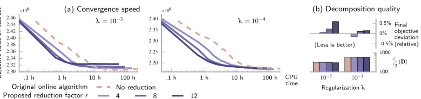
Figure 1. Acceleration of sparse matrix factorizationwith random subsampling on the HCP dataset (2TB). Reducing streamed data
with stochastic masks permits10×speed-ups without deteriorating goodness of fit on test data nor alterating sparsity of final dictionary.
we analyze in detail how our algorithm improves perfor-mance for sparse decomposition of fMRI datasets. More-over, as it relies on data masks, our algorithm is well suited for matrix completion, to reconstruct a data stream (xt)t from the masked stream(Mtxt)t. We demonstrate the ac-curacy of our algorithm on explicit recommender systems and show considerable computational speed-ups compared to an efficient coordinate-descent based algorithm. We usescikit-learn(Pedregosa et al.,2011) in experiments, and have released a python package1for reproducibility.
3.1. Sparse Matrix Factorization for fMRI
Context. Matrix factorization has long been used on functional Magnetic Resonance Imaging (McKeown et al.,
1998). Data are temporal series of 3D images of brain ac-tivity, to decompose in spatial modes capturing regions that activate together. The matrices to decompose are dense and heavily redundant, both spatially and temporally: close voxels and successive records are correlated. Data can be huge: we use the whole HCP dataset (Van Essen et al.,
2013), withn= 2.4·106(2000 records, 1 200 time points)
andp= 2·105, totaling 2 TB of dense data.
Interesting dictionaries for neuroimaging capture spatially-localized components, with a few brain regions. This can be obtained by enforcing sparsity on the dictionary: in our formalism, this is achieved with`1-ball projection forD.
We setC=Bk
1, andΩ =k · k22. Historically, such
decom-position have been obtained with the classical dictionary learning objective on transposed data (Varoquaux et al.,
2013): the code A holds sparse spatial maps and voxel
time-series are streamed. However, given the size ofnfor
our dataset, this method is not usable in practice.
Handling such volume of data sets new constraints. First, efficient disk access becomes critical for speed. In our case, learning the dictionary is done by accessing the data in row batches, which is coherent with fMRI data storage: no time is lost seeking data on disk. Second, reducing IO load on
1http://github.com/arthurmensch/modl
the storage is also crucial, as it lifts bottlenecks that appear when many processes access the same storage at the same time,e.g. during cross-validation onλwithin a supervised
pipeline. Our approach reduces disk usage by a factorr.
Finally, parallel methods based on message passing, such as asynchronous coordinate descent, are unlikely to be effi-cient given the network / disk bandwidth that each process requires to load data. This makes it crucial to design effi-cient sequential algorithms.
Experiment We quantify the effect of random subsam-pling for sparse matrix factorization, in term of speed and accuracy. A natural performance evaluation is to measure an empirical estimate of the loss l defined in Eq.4 from
unseendata, to rule out any overfitting effect. For this, we evaluatelon a test set(xi)i<N. Pratically, we sample(xt)t in a pseudo-random manner: we randomly select a record, from where we select a random batch of rowsxt– we use a batch size of40, empirically found to be efficient. We
loadMtxtin memory and perform an iteration of the algo-rithm. The mask sequence is sampled by breaking random permutation vectors into chunks of sizep/r.
Results Fig.1(a) compares our algorithm with subsam-pling ratios r in {4,8,12} to vanilla online dictionary learning algorithm (r = 1), plotting trajectories of the
testobjective against real CPU time. There is no obvious choice ofλdue to the unsupervised nature of the problem: we use10−3and10−4, that bounds the range ofλ
provid-ing interpretable dictionaries.
First, we observe the convergence of the objective func-tion for all testedr, providing evidence that the
approx-imations made in the derivation of update rules does not break convergence for suchr. Fig.1(b) shows the validity
of the obtained dictionary relative to the reference output: both objective function and`1/`2ratio – the relevant value
to measure sparsity in our setting – are comparable to the baseline values, up tor = 8. For high regularization and
r= 12, our algorithm tends to yield somewhat sparser
so-lutions (5%lower`1/`2) than the original algorithm, due to
235 hrun time
Original online algorithm 1 full epoch
10 hrun time
Original online algorithm
1 24epoch 10 hrun time Proposed algorithm 1 2epoch, reductionr=12
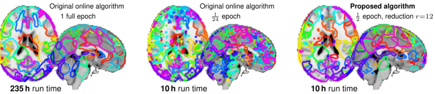
Figure 2.Brain atlases: outlines of each map at half the maximum value (λ= 10−4).Left: the reference algorithm on the full dataset.
Middle: the reference algorithm on a twentieth of the dataset. Right: the proposed algorithm with a similar run time: half the dataset andr= 9. Compared to a full run of the baseline algorithm, the figure explore two possible strategies to decrease computation time:
processing less data (middle), or our approach (right). Our approach achieves a result closer to the gold standard in a given time budget.
100 1000 Epoch 4000 Records2.16 2.17 2.18 2.19 2.20 2.21 2.22 2.23 2.24 Objective value on test set × 108 λ=10−4 No reduction (original alg.) r=4 r=8 r=12
Figure 3.Evolution of objective function with epochsfor three
reduction factors. Learning speed per epoch is little reduced by stochastic subsampling, despite the speed-up factor it provides.
still proves as interpretable as with baseline algorithm. Our algorithm proves much faster than the original one in finding a good dictionary. Single iteration time is indeed reduced by a factorr, which enables our algorithm to go
over a single epoch r times faster than the vanilla
algo-rithm and capture the variability of the dataset earlier. To quantify speed-ups, we plot the empirical objective value of D against the number of observed records in Fig. 3.
Forr ≤12, increasingrlittle reduces convergence speed
per epoch: random subsampling does not shrink much the quantity of information learned at each iteration.
This brings a near ×r speed-up factor: for high and low regularization respectively, our algorithm converges in 3
and10hours with subsampling factorr= 12, whereas the vanilla online algorithm requires about30and100hours.
Qualitatively, Fig.2shows that with the same time budget, the proposed reduction approach withr = 12on half of
the data gives better results than processing a small frac-tion of the data without reducfrac-tion: segmented regions are less noisy and closer to processing the full data.
These results advocates the use of a subsampling rate of
r≈10in this setting. When sparse matrix decomposition
is part of a supervised pipeline with scoring capabilities, it is possible to findrefficiently: start by setting it derea-sonably high and decrease it geometrically until supervised
performance (e.g.in classification) ceases to improve.
3.2. Collaborative Filtering with Missing Data
We validate the performance of the proposed algorithm on recommender systems for explicit feedback, a well-studied matrix completion problem. We evaluate the scalability of our method on datasets of different dimension: MovieLens 1M, MovieLens 10M, and 140M ratings Netflix dataset. We compare our algorithm to a coordinate-descent based method (Yu et al.,2012), that provides state-of-the art con-vergence time performance on our largest dataset. Al-though stochastic gradient descent methods for matrix fac-torization can provide slightly better single-run perfor-mance (Takács et al.,2009), these are notoriously hard to tune and require a precise grid search to uncover a working schedule of learning rates. In contrast, coordinate descent methods do not require any hyper-parameter setting and are therefore more efficient in practice. We benchmarked var-ious recommender-system codes (MyMediaLite, LibFM,
SoftImpute, spira2), and chose coordinate descent
algo-rithm fromspiraas it was by far the fastest.
Completion from dictionaryDt. We stream user ratings to our algorithm: pis the number of movies andnis the
number of users. Asn pon Netflix dataset, this in-creases the benefit of using an online method. We have ob-served comparable prediction performance streaming item ratings. Past the first epoch, at iterationt, every columni
ofXcan be predicted by the last codeαl(i,t)that was
com-puted from this column at iterationl(i, t). At iterationt, for alli <[n],xpredi =Dαl(i,t). Prediction thus only requires
an additional matrix computation after the factorization.
Preprocessing. Successful prediction should take into account user and item biases. We compute these biases on train data followingHastie et al.(2014) (alternated
0.1 s 1 s 10 s 0.87 0.88 0.89 0.90 0.91 RMSE on test set MovieLens 1M 1 s 10 s 100 s 0.80 0.81 0.82 0.83 0.84 0.85 0.86 MovieLens 10M 100 s 1000 s CPU time 0.93 0.94 0.95 0.96 0.97 0.98
0.99 Netflix (140M) Coordinate descent Proposed
(full projection) Proposed (partial projection)
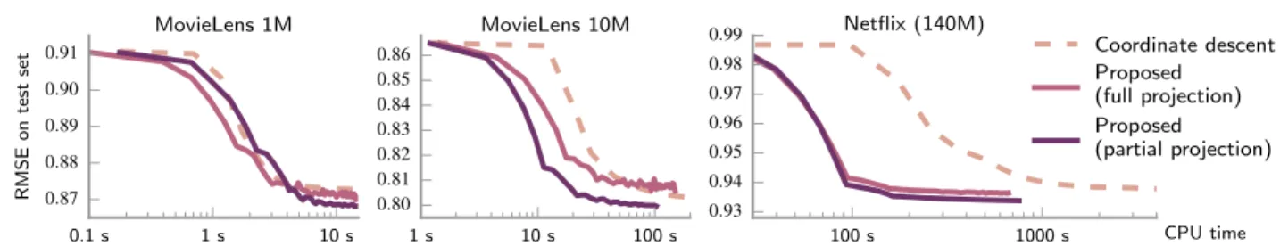
Figure 4.Learning speed for collaborative filteringfor datasets of different size: the larger the dataset, the greater our speed-up.
Table 1.Comparison of performance and convergence time
for online masked matrix factorization and coordinate descent method. Convergence time: score is under 0.1% deviation from final root mean squared error on test set – 5 runs average. CD: coordinate descent; MODL: masked online dictionary learning.
Dataset Test RMSE Convergence time Speed
CD MODL CD MODL -up
ML 1M 0.872 0.866 6 s 8s ×0.75
ML 10M 0.802 0.799 223s 60 s ×3.7
NF (140M) 0.938 0.934 1714s 256 s ×6.8
biasing). We use them to center the samples(xt)tthat are streamed to the algorithm, and to perform final prediction.
Tools and experiments. Both baseline and proposed al-gorithm are implemented in a computationally optimal way, enabling fair comparison based on CPU time. Bench-marks were run using a single 2.7 GHz Xeon CPU, with a 30 components dictionary. For Movielens datasets, we use a random25%of data for test and the rest for training.
We average results on five train/test split for MovieLens in Table1. On Netflix, the probe dataset is used for testing. Regularization parameterλis set by cross-validation on the
training set: the training data is split 3 times, keeping33%
of Movielens datasets for evaluation and 1% for Netflix, and grid search is performed on 15 values of λbetween
10−2 and10. We assess the quality of obtained
decom-position by measuring the root mean square error (RMSE) between prediction on the test set and ground truth. We use mini-batches of size n
100.
Results. We report the evolution of test RMSE along time in Fig.4, along with its value at convergence and numerical convergence time in Table1. Benchmarks are performed on the final run, after selection of parameterλ.
The two variants of the proposed method converge toward a solution that is at least as good as that of coordinate de-scent, and slightly better on Movielens 10M and Netflix. Our algorithm brings a substantial performance improve-ment on medium and large scale datasets. On Netflix, con-vergence is almost reached in4minutes (score under0.1%
deviation from final RMSE), which makes our method6.8
times faster than coordinate descent. Moreover, the relative performance of our algorithm increases with dataset size. Indeed, as datasets grow, less epochs are needed for our algorithm to reach convergence (Fig.4). This is a signifi-cant advantage over coordinate descent, that requires a sta-ble number of cycle on coordinates to reach convergence, regardless of dataset size. The algorithm with partial pro-jection performs slightly better. This can be explained by the extra regularization on(Dt)tbrought by this heuristic.
Learning weights. Unlike SGD, and similar to the vanilla online dictionary learning algorithm, our method does not critically suffer from hyper-parameter tuning. We tried weights wt = t1β as described in Sec.2.3, and ob-served that a range of β yields fast convergence. Theo-retically,Mairal(2013) shows that stochastic majorization-minimization converges whenβ ∈ (.75,1]. We verify
this empirically, and obtain optimal convergence speed for
β ∈[.85,0.95]. (Fig.5). We report results forβ = 0.9.
1 10 40 Epoch 0.80 0.81 0.82 0.83 0.84 0.85 0.86 0.87 RMSE on test set Learning rateβ 0.75 0.78 0.81 0.83 0.86 0.89 0.92 0.94 0.97 1.00 MovieLens 10M .1 1 10 20 0.93 0.94 0.95 0.96 0.97 0.98 0.99 Netflix
Figure 5.Learning weights: on two different datasets, optimal
convergence is obtained forβ∈[.85, .95], predicted by theory.
4. Conclusion
Whether it is sensor data, as fMRI, or e-commerce databases, sample sizes and number of features are rapidly growing, rendering current matrix factorization approaches intractable. We have introduced a online algorithm that leverages random feature subsampling, giving up to 8-fold speed and memory gains on large data. Datasets are getting bigger, and they often come with more redundancies. Such approaches blending online and randomized methods will yield even larger speed-ups on next-generation data.
Acknowledgements
The research leading to these results was supported by the ANR (MACARON project, ANR-14-CE23-0003-01 – NiConnect project, ANR-11-BINF-0004NiConnect) and has received funding from the European Union Sev-enth Framework Programme (FP7/2007-2013) under grant agreement no. 604102 (HBP).
References
Aharon, Michal, Elad, Michael, and Bruckstein, Alfred. k-SVD: An algorithm for designing overcomplete dictio-naries for sparse representation. IEEE Transactions on Signal Processing, 54(11):4311–4322, 2006.
Bell, Robert M. and Koren, Yehuda. Lessons from the Netflix prize challenge. ACM SIGKDD Explorations Newsletter, 9(2):75–79, 2007.
Bingham, Ella and Mannila, Heikki. Random projection in dimensionality reduction: applications to image and text data. InProceedings of ACM SIGKDD International Conference on Knowledge Discovery and Data Mining, pp. 245–250. ACM, 2001.
Blondel, Mathieu, Fujino, Akinori, and Ueda, Naonori. Convex factorization machines. In Machine Learning and Knowledge Discovery in Databases, pp. 19–35. Springer, 2015.
Bottou, Léon. Large-scale machine learning with stochas-tic gradient descent. InProceedings of COMPSTAT, pp. 177–186. Springer, 2010.
Candès, Emmanuel J. and Recht, Benjamin. Exact ma-trix completion via convex optimization. Foundations of Computational Mathematics, 9(6):717–772, 2009. Candès, Emmanuel J. and Tao, Terence. Near-optimal
sig-nal recovery from random projections: Universal encod-ing strategies? Information Theory, IEEE Transactions on, 52(12):5406–5425, 2006.
Duchi, John, Shalev-Shwartz, Shai, Singer, Yoram, and Chandra, Tushar. Efficient projections onto the l 1-ball for learning in high dimensions. InProceedings of the International Conference on Machine Learning, pp. 272–279. ACM, 2008.
Halko, Nathan, Martinsson, Per-Gunnar, and Tropp, Joel A. Finding structure with randomness: Probabilistic algorithms for constructing approximate matrix decom-positions.arXiv:0909.4061 [math], 2009.
Hastie, Trevor, Mazumder, Rahul, Lee, Jason, and Zadeh, Reza. Matrix completion and low-rank SVD via fast al-ternating least squares.arXiv:1410.2596 [stat], 2014.
Johnson, William B. and Lindenstrauss, Joram. Extensions of Lipschitz mappings into a Hilbert space. Contempo-rary mathematics, 26(189-206):1, 1984.
Mairal, Julien. Stochastic majorization-minimization al-gorithms for large-scale optimization. In Advances in Neural Information Processing Systems, pp. 2283–2291, 2013.
Mairal, Julien. Sparse Modeling for Image and Vision Pro-cessing. Foundations and Trends in Computer Graphics and Vision, 8(2-3):85–283, 2014.
Mairal, Julien, Bach, Francis, Ponce, Jean, and Sapiro, Guillermo. Online learning for matrix factorization and sparse coding. The Journal of Machine Learning Re-search, 11:19–60, 2010.
McKeown, M. J., Makeig, S., Brown, G. G., Jung, T. P., Kindermann, S. S., Bell, A. J., and Sejnowski, T. J. Anal-ysis of fMRI Data by Blind Separation into Independent Spatial Components.Human Brain Mapping, 6(3):160– 188, 1998. ISSN 1065-9471.
Pedregosa, Fabian, Varoquaux, Gaël, Gramfort, Alexan-dre, Michel, Vincent, Thirion, Bertrand, Grisel, Olivier, Blondel, Mathieu, Prettenhofer, Peter, Weiss, Ron, Dubourg, Vincent, Vanderplas, Jake, Passos, Alexan-dre, Cournapeau, David, Brucher, Matthieu, Perrot, Matthieu, and Duchesnay, Édouard. Scikit-learn: ma-chine learning in Python. Journal of Machine Learning Research, 12:2825–2830, 2011.
Pourkamali-Anaraki, Farhad, Becker, Stephen, and Hughes, Shannon M. Efficient dictionary learning via very sparse random projections. InProceedings of the IEEE International Conference on Sampling Theory and Applications, pp. 478–482. IEEE, 2015.
Rendle, Steffen. Factorization machines. InProceedings of the IEEE International Conference on Data Mining, pp. 995–1000. IEEE, 2010.
Rendle, Steffen and Schmidt-Thieme, Lars. Online-updating regularized kernel matrix factorization models for large-scale recommender systems. In Proceedings of the ACM Conference on Recommender systems, pp. 251–258. ACM, 2008.
Srebro, Nathan, Rennie, Jason, and Jaakkola, Tommi S. Maximum-margin matrix factorization. InAdvances in Neural Information Processing Systems, pp. 1329–1336, 2004.
Szabó, Zoltán, Póczos, Barnabás, and Lorincz, András. Online group-structured dictionary learning. In Proceed-ings of the IEEE Conference on Computer Vision and Pattern Recognition, pp. 2865–2872. IEEE, 2011.
Takács, Gábor, Pilászy, István, Németh, Bottyán, and Tikk, Domonkos. Scalable collaborative filtering approaches for large recommender systems.The Journal of Machine Learning Research, 10:623–656, 2009.
Van Essen, David C., Smith, Stephen M., Barch, Deanna M., Behrens, Timothy E. J., Yacoub, Essa, and Ugurbil, Kamil. The WU-Minn Human Connectome Project: An overview.NeuroImage, 80:62–79, 2013. Varoquaux, Gaël, Gramfort, Alexandre, Pedregosa, Fabian,
Michel, Vincent, and Thirion, Bertrand. Multi-subject dictionary learning to segment an atlas of brain sponta-neous activity. InProceedings of the Information Pro-cessing in Medical Imaging Conference, volume 22, pp. 562–573. Springer, 2011.
Varoquaux, Gaël, Schwartz, Yannick, Pinel, Philippe, and Thirion, Bertrand. Cohort-level brain mapping: learn-ing cognitive atoms to slearn-ingle out specialized regions. In
Proceedings of the Information Processing in Medical Imaging Conference, pp. 438–449. Springer, 2013. Yu, Hsiang-Fu, Hsieh, Cho-Jui, and Dhillon, Inderjit.
Scal-able coordinate descent approaches to parallel matrix factorization for recommender systems. InProceedings of the International Conference on Data Mining, pp. 765–774. IEEE, 2012.