Institut d’Economie Industrielle (IDEI)– Manufacture des Tabacs
February, 2009
n° 635
“Log-Density Deconvolution by
Wavelet Thresholding”
Jérôme BIGOT and
Sébastien VAN BELLEGEM
LOG
-DENSITY DECONVOLUTION
BY WAVELET THRESHOLDING
J´er´emie Bigot & S´ebastien Van Bellegem
This version: February, 11, 2009
Abstract
This paper proposes a new wavelet-based method for deconvolving a density. The estimator combines the ideas of nonlinear wavelet thresholding with periodised Meyer wavelets and estimation by information projection. It is guaranteed to be in the class of density functions, in particular it is positive everywhere by construction. The asymptotic optimality of the estimator is established in terms of rate of convergence of the Kullback-Leibler discrepancy over Besov classes. Finite sample properties is investigated in detail, and show the excellent empirical performance of the estimator, compared with other recently introduced estimators.
Keywords:Deconvolution, Wavelet thresholding, Adaptive estimation, Information projection, Kullback-Leibler divergence, Besov space
AMS classifications:Primary 62G07; secondary 42C40, 41A29
Affiliations
J ´EREMIE´ BIGOT, Institut de Math´ematiques de Toulouse, Universit´e de Toulouse et CNRS (UMR 5219), F-31062 Toulouse Cedex 9, France,[email protected]
S ´EBASTIENVANBELLEGEM, Toulouse School of Economics (Gremaq), 21, All´ee de Brienne, F-31200 Toulouse, France,[email protected]
Ackowledgements
This work was supported by the IAP research network nr P5/24 of the Belgian Government (Belgian Science Policy). We gratefully ackowledge Yves Rozenholc for providing the Matlab code to compute
the model selection estimator, Marc Raimondo for providing the Matlab code for translation invariant deconvolution, and Anestis Antoniadis for helpful comments .
1
Introduction
Density deconvolution arises when the probability density of a random variable X
has to be estimated from an independent and identically distributed (iid) sample contaminated by some independent additive noise. Namely, the observations at hand, denoted byYi fori = 1, . . . ,n, are such thatYi =Xi+ǫi,i = 1, . . . ,n, whereXi are iid
variables with unknown density fX, andǫiis an additive random error. The numbern
represents the sample size and the contamination variables ǫi are supposed iid with a
known density function fǫ, and independent from theXi’s. In this setting, the density
function fY of the observed sample Yi can be written as a convolution between the
density of interest fX, and the density of the additive noise fǫ, i.e.
fY(y) = fX⋆ fǫ(y) :=
Z
fX(u)fǫ(y−u)du, y ∈R . (1.1)
The problem of estimating the probability density fX relates to classical
nonparametric methods of estimation, but the indirect observation of the data leads to different optimality properties, for instance in terms of rate of convergence. Among the nonparametric methods of deconvolution, one can find estimation by model selection
(e.g. Comte et al., 2006), wavelet thresholding (e.g. Fan and Koo, 2002), kernel
smoothing (e.g. Carroll and Hall, 1988), spline deconvolution (e.g. Koo, 1999) or
spectral cut-off (e.g. Johanneset al., 2007). However, a problem frequently encountered
is that the proposed estimator is not everywhere positive, therefore is not a valid probability density. The main goal of the present paper is to introduce an estimator that is automatically a valid density, in particular because it is guaranteed to be positive. The proposed solution uses wavelet thresholding combined with information projection techniques, and is computationally simple.
The advantage of wavelet methods is their ability in estimating local features of the density, such as peaks or local discontinuities. Wavelet methods for deconvolution have received a special attention in the recent literature. Optimality of the nonlinear wavelet estimator has been established in Fan and Koo (2002), but the given estimator is not computable since it depends on an integral in the frequency domain that cannot
be calculated in practice. Other wavelet estimators are presented in Johnstone et
al. (2004) and De Canditiis and Pensky (2006), see also the references therein. Our
estimator combines wavelet thresholding with information projection that guarantees the solution to be positive. This technique was studied by Barron and Sheu (1991) for the approximation of density functions by sequences of exponential families. An extension of this method to linear inverse problems has been studied in Koo and Chung (1998) using expansions in Fourier series.
It is well-known that the difficulty of the deconvolution problem is quantified by
the smoothness of the noise density fǫ. If fℓY, fℓXand fℓǫ denote the Fourier coefficients
of the densities fY, fX and fǫ respectively, then the convolution equation (1.1) is
equivalent to fℓY = fℓX· fℓǫ. Depending how fast the Fourier coefficients fℓǫtend to zero,
the reconstruction of fℓX will be more or less accurate. In this paper, we consider the
case where the fℓǫ’s have a polynomial decay which is usually referred to as ordinary
smooth convolution (see e.g. Fan (1991)):
Assumption 1.1 The Fourier coefficients of fǫ decay at a polynomial rate i.e. there exist constants c1,c2 >0and a realν>0such that c1|ℓ|−ν 6|fℓǫ|6c2|ℓ|−ν.
TheL2-rate of convergence that can be expected from a linear or a nonlinear wavelet
estimator depends on this assumption and are well-studied in the literature, see e.g. Pensky and Vidakovic (1999); Fan and Koo (2002).
After recalling some general results on Meyer wavelets, we define in Section 3 our linear and nonlinear wavelet estimators by information projection. This paper demonstrates two important features of the non linear estimator. First we prove in Section 4 that its asymptotic rate of convergence, measured in the
Kullback-Leibler divergence, is optimal over Besov balls Fps,q(M) (defined below). Moreover,
the resulting estimator is positive by construction and shows excellent finite sample properties. As we show in Section 5, it outperforms some of the best nonparametric estimators recently published in the literature.
2
Meyer wavelets for deconvolution
In this paper, we assume that the support of fX is compact and included in[0, 1]. Of
it is mainly made for mathematical convenience.
Wavelet systems provide unconditional bases for Besov spaces. Using wavelets,
one can characterize whether or not fX belongs to a Besov space by a condition
on the absolute value of the wavelet coefficients of fX. Assume that (φ,ψ) denotes
some scaling and wavelet functions that have enough regularity and vanishing
moments. Let s ≥ 0, p,q ≥ 1, and if σ = s+ (1/2−1/p) > 0, define the norm
kfXkqs,p,q = ∑∞j=0(2jσp∑2
j−1
k=0 |hfX,ψj,ki|p)q/p. It can be shown (Meyer, 1992) that this
norm is equivalent to the norm in the Besov space Bsp,q. The parameter s is related
to the smoothness of fX. In particular if fX is piecewise Cα with a finite number of
discontinuities, then fX belongs toBsp,q for alls <αand psufficiently small.
The estimator we shall define in the next section is based on the wavelet
decomposition of functions in L2([0, 1]) using periodised Meyer wavelets. This
wavelet basis is derived through the periodisation of the Meyer wavelet basis ofL2(R).
This basis is constructed from a scaling functionφwith Fourier transform
˜ φ(ω) = ( ˜ h(ω/2)/√2 if |ω| 64π/3, 0 if |ω| >4π/3,
where ˜h : C → R is a smooth function (see Meyer (1992), Johnstone et al. (2004) for
further details). In the simulations below, ˜h is a cubic function known as the Meyer
window(e.g. Mallat, 1998, p. 248).
Meyer wavelets are therefore band-limited which makes them very useful for
deconvolution problems. Indeed, let (φ,ψ) be the periodised Meyer scaling and
wavelet function respectively. Scaling and wavelet functions at scale j (i.e. resolution
level 2j) will be denoted byφλ andψλ, where the indexλsummarizes both the usual
scale and space parameters j and k (i.e. λ = (j,k) and ψj,k = 2j/2ψ(2j· −k)). The
notation |λ| = j will be used to denote a wavelet at scale j, while |λ| < j denotes
some wavelet at scale j′, with 0 6 j′ < j. For any function fX of L2([0, 1]), its
wavelet decomposition can be written as fX =∑|λ|=j
0cλφλ+∑ ∞ j=j0∑|λ|=jβλψλ, where cλ = hfX,φλi = R1 0 fX(u)φλ(u)du, βλ = hfX,ψλi = R1 0 fX(u)ψλ(u)du and j0denotes
the usual coarse level of resolution. Let eℓ(x) = exp(2πiℓx), ℓ ∈ Z and denote by
fℓX = hfX,eℓithe Fourier coefficients of a function fX ∈ L2([0, 1]). Then, if we denote
the Fourier coefficients ofψλbyψλℓ =hψλ,eℓiwe obtain with the Plancherel’s identity
Given that the Meyer wavelets ψλ are band-limited, the above sum only involves
a finite number of terms. Now, if we denote by fℓǫ = E(e−2πi
ℓǫ1
) the characteristic
function of theǫj’s and by fℓY = E(e−2πi ℓY1
)the characteristic function of theYj’s , we
have by independence ofX1 andǫ1that fℓY =E(e−2πi
ℓY1
) =E(e−2πiℓǫ1)E(e−2πiℓX1) =
fℓǫfℓX. An unbiased estimator ofβλ is thus given by
ˆ βλ =
∑
ℓ ψλℓ fǫ ℓ ! 1 n n∑
j=1 exp(−2πiℓYj) ! . (2.1)provided that the fǫ
ℓ’s are non-zero and have a sufficiently smooth decay asℓtends to
infinity. Analogously the estimators of the scaling coefficients cλ is defined using the
scaling functionφinstead ofψ.
3
Estimation by information projection
3.1
Linear and nonlinear wavelet estimators
Based on the coefficients ˆcλand ˆβλ, several estimators of the unknown density fX can
be studied. First of all, the linear estimator is such that ˆ fLX =
∑
|λ|=j0 ˆ cλφλ+ j1∑
j=j0∑
|λ|=j ˆ βλψλThis estimator was first studied by Pensky and Vidakovic (1999), who showed that for
an appropriate scalej1, it achieves the optimal rate of convergence among the class of
linear estimators. In the ordinary smooth situation (Assumption 1.1), the choice of j1
is such that 2j1 = O(n1/2s+2ν+1) if fX belongs to the Sobolev space Hs. Note that this
choice is not adaptive becausej1depends on the unknown smoothness class of fX.
In contrast, adaptive nonlinear estimators by wavelet thresholding have been developed and they can achieve near-optimal rate of convergence (up to logarithmic
factors). To simplify the notations, hereafter we write (ψλ)|λ|=j0−1 for the scaling
functions(φλ)|λ|=j0. A non-linear estimator is defined by
ˆ fhX = j1
∑
j=j0−1∑
|λ|=j δτhj,n(βˆλ)ψλwithδτhj,n(x) = x11{|x|>τj,n}. This estimator depends on the coarse level of approximation
j0, the high-frequency cut-off j1 and the thresholdτj,n that may depend on the level of
resolution j. An adaptive estimator is derived with appropriate choices of scalesj0, j1
and threshold. One possible calibration for an adaptive estimator in ordinary smooth
deconvolution is 2j1 = O(n1/2ν+1) and δ
j,n = O(2νj/√n) (Pensky and Vidakovic,
1999). The choiceδj,n =O(2νj
p
j/n)has also been considered (Fan and Koo, 2002).
3.2
Information projection to guarantee positivity
Letj >0. Ifθdenotes a vector inR2j, thenθλ denotes itsλ-th component. The wavelet
based exponential familyEjat scalejis defined as the set of functions:
Ej = n fj,θ(·) =exp(
∑
|λ|<j θλψλ(·)−Cj(θ)), θ = (θλ)|λ|<j ∈ R2 jo , where Cj(θ) = log R10 exp(∑|λ|<jθλψλ(x))dx. Following Csisz´ar (1975), the density
function fj,θ inEjthat is the closest to the true density fXin the Kullback-Leibler sense
is the unique density function in Ej for which hfj,θ,ψλi = hfX,ψλi, for all|λ| < j. It
seems therefore natural to estimate the unknown density function fX, by looking for
some ˆθn ∈ R2 j such that: hfj, ˆθn,ψλi =
∑
ℓ ψlλ fǫ l ! 1 n n∑
j=1 exp(−2πiℓYj) ! :=αˆλ, for all|λ|< j. (3.1)Note that the notation ˆαλ is used to denote both the estimation of the scaling
coefficients ˆcλand the wavelet coefficients ˆβλ.
The positive linear and nonlinear wavelet estimator are then defined as follows: • Thepositive linear wavelet estimatoris fj
1, ˆθnsuch thathfj1, ˆθn,ψλi =αˆλfor all|λ|< j1
• Thepositive nonlinear estimator with hard thresholdingis fh
j1, ˆθn such thathf
h
j1, ˆθn,ψλi=
δτhj,n(αˆλ)for all|λ| <j1
The existence of these estimators is questionable. This issue is addressed in the next section and in the technical appendix. Moreover, there is no way to obtain an explicit
expression for ˆθn. In our simulations, we use a numerical approximation of ˆθn that is
4
Rates of convergence of the estimators
Below we study the convergence of the estimators for the Kullback-Leibler discrepancy
loss between two probability density functions pandq, that is given by:
∆(p;q) =
Z 1
0 p(x)log(
p(x)
q(x))dx,
where dx denotes the Lebesgue measure on [0, 1]. Let M be some fixed constant
and let Fps,q(M) denote the set of density functions such that Fps,q(M) = {f ∈
L2[0, 1]is a p.d.f. such that forg=log f, kgkqs,p,q 6 M}.
4.1
Linear estimation
The following theorem is about the nonadaptive information projection estimator of the unknown density function.
Theorem 4.1 Assume fX ∈ F2,2s (M) with s > 1, and suppose that the convolution kernel
fǫ satisfies Assumption 1.1 (ordinary smooth convolution). Let j(n) be such that2−j(n) = O(n−1/(2s+2ν+1)). Then, the information projection estimator fj(n), ˆθ
n exists with probability
tending to one as n→+∞, and is such that
E∆fX; f j(n), ˆθn =On−2s+22sν+1 .
In the case of ordinary smooth deconvolution, Koo and Chung (1998) have shown
thatn−2s+22sν+1 is the fastest rate of convergence for the problem of estimating a density
f such that log(f) belongs to Sobolev ball of order s which corresponds to the space
F2,2s (M). The above estimator fj(n), ˆθ
n therefore converges with the optimal rate for
densities in F2,2s (M). However, this estimator is not adaptive since the choice of j(n)
depends on the unknown smoothness class of the function fX. Moreover, the result is
only suited for smooth functions (asF2,2s (M)corresponds to a Sobolev space of orders)
and does not attain the optimal rates when for exampleg =log(fX)has singularities.
In the next section, we therefore propose another estimator based on an appropriate nonlinear thresholding procedure.
4.2
Non-linear estimation
In non-linear estimation, we need to define an appropriate thresholding of the
estimated coefficients ˆαλ. This threshold is level-dependent and takes the form τj,n =
ητj
p
(logn)/nwith τj =2jν, and for some constantη >0. The size of the exponential
family used for the estimation depends on the high-frequency cut-off j1 which is
typically related to the ill-posedness ν of the inverse problem e.g. 2j1 > n1/2ν as in
Antoniadis and Bigot (2006) or 2j1 =O
(logn(n))1/(2ν+1)as in Johnstoneet al. (2004).
The following theorem gives the rate of convergence of the expected Kullback-Leibler discrepancy for the positive nonlinear estimator by hard thresholding.
Theorem 4.2 Assume that fX ∈ Fps,q(M), and suppose that the convolution kernel fǫsatisfies Assumption 1.1 withν>0(ordinary smooth convolution). Suppose
06q6min((4ν+2)/(2s+2ν+1), 4ν/(2s+2ν−2/p+1))
16p 62, s>1/p+1/2, ν>1/2, (4.1)
s>(2ν+1)(1/p+1/2), s >1/2+1/(4ν) (4.2)
Then, the above described hard thresholding estimator exists with probability tending to one as n →+∞, and satisfies E∆(fX; fh j1(n), ˆθn) =O logn n 2s/(2s+2ν+1)! ,
provided that2j1(n) =O((n/log(n))1/(2ν+1)).
The space Fps,q(M) with 1 6 p < 2 contains piecewise smooth functions with
local irregularities such as peaks or discontinuities. In the classical density estimation problem (without an additive noise), Koo and Kim (1996) have studied the optimal rate of convergence in the minimax sense for the Kullback-Leibler discrepancy over the density class Fps,q(M). It is shown in Koo and Kim (1996) that n−2s/(2s+1) is the
lowest rate of convergence if s > 1/2 and p,q > 1. However, to the best of our
knowledge, studying optimal rates of convergence for ordinary smooth deconvolution
has not been investigated for the Kullback-Leibler discrepancy for the class Fps,q(M).
We conjecture that n−2s/(2s+2ν+1) is a lower bound for the problem of estimating
0 0.2 0.4 0.6 0.8 1 0 1 2 3 4 5 6 (a) 0 0.2 0.4 0.6 0.8 1 0 2 4 6 8 10 (b) 0 0.2 0.4 0.6 0.8 1 0 2 4 6 8 10 (c) 0 0.2 0.4 0.6 0.8 1 0 1 2 3 4 5 (d)
Figure 5.1: Test densities: (a) Uniform, (b) Exponential, (c) Laplace, (d) MixtGauss (mixture of two Gaussian)
shows that our information projection estimate based on hard thresholding is adaptive
and converges with a near-optimal rate. Note that in Johnstone et al. (2004), the case
1/p−1/2−ν 6s <(2ν+1)(1/p−1/2) is also considered for which a different rate
of convergence is derived. This is known as the ’Elbow’ phenomenon which has been
commonly observed in direct models and recently noticed by Johnstone et al. (2004)
for deconvolution problems, but for simplicity we have not considered this case. The conditions (4.1) and (4.2) in particular guarantee the existence with probability tending to one of the information projection estimates, see the proof of Theorem 4.2 where Lemma 5 of Barron and Sheu (1991) is also used. Moreover, note that our
condition on the high-frequency cut-off yields a choice for j1 which is similar to the
one obtained by the conditions in Johnstoneet al. (2004). The problem of determining
the choice ofj1in practice is further discussed in the next section.
5
Simulations
Given a density fX with variance σX2 and a noise density fǫ with variance σ2
ǫ we
generate observations Yi,i = 1, . . . ,n from the additive model Yi = Xi +ǫi, where
Xi (resp. ǫi) are independent realizations from fX (resp. fǫ). Important quantities
in the simulations are the sample size n and the root signal-to-noise ratio defined by
s2n := σX/σǫ. For the sake of conciseness, we only present results with a Laplace
measurement error, that is fǫ(x) = (√2σ
ǫ)−1exp(− √
2|x|/σǫ), x ∈ R. The Fourier
coefficients of this density are given by fℓǫ = (1+2σǫ2π2ℓ2)−1, ℓ = 0,±1,±2, . . .. This
noise density corresponds to the case of ordinary smooth deconvolution withν =2.
The Uniform distribution f(x) = 511[0.4,0.6](x); the Exponential distribution f(x) =
10e−10(x−0.2)11[0.2,+∞[(x); (3) the Laplace distribution f(x) = 10e−20|x−0.5| and (4)
the MixtGauss distribution which is a mixture of two Gaussian variables i.e. X ∼
π1N(µ1,σ12) +π2N(µ2,σ22)with π1 = 0.4,π1 = 0.6,µ1 = 0.4,µ2 = 0.6 andσ1 = σ2 =
0.05. The four densities fXare displayed in Figure 5.1, where we can observe that they
show various types of smoothness. The Uniform distribution is a piecewise constant function with two jumps, the Exponential distribution is a piecewise smooth function
with a single jump, the Laplace density is a continuous function with a cusp atx=0.5
and is thus non-differentiable at this point, whereas the MixtGauss density is infinitely differentiable.
5.1
Computation of the estimators
The computation of the wavelet deconvolution by information projection is described below. It is compared with two among the most recent estimators found in the literature : the estimator by model selection of Comte, Rozenholc and Taupin (2007) and cosine series deconvolution of Hall and Qiu (2005). Simulations use the wavelet
toolboxWavelabof Matlab (Buckheitet al., 1995).
5.1.1 Wavelet deconvolution
The empirical Fourier coefficients ∑nj=1exp(−2πiℓYj)/(n fℓǫ) are computed for ℓ =
−n/2+1, . . . ,n/2. They are used as an input of the efficient algorithm of Kolaczyk
(1994) in order to compute the Meyer wavelet coefficients of a discrete signal.
According to Theorem 4.2, the optimal cut-off is j∗1 = (2ν+1)−1log2(n). As we
will show below, this choice is too small in practice. However, this choice is crucial because a too high level of resolution might unacceptably introduce instability in the estimator (for instance when a large wavelet coefficient due to the noise at a fine scale is erroneously kept by the thresholding procedure). One objective of the simulation
study is to identify a reasonable empirical range of scales j1. We will investigate every
possible values ofj1between 3 and log2(n)−1.
For a non linear wavelet estimator, Theorem 4.2 suggests to set the threshold
τj,n = ητjp(logn)/n, where η is a tuning constant andτj = 2jν. Based on extensive
(universal thresholding). In the context of Meyer wavelet-based deconvolution in
a regression setting, Johnstone et al. (2004) use the same type of level-dependent
thresholding but the scale parameter τj depends on the noise distribution fǫ and
on the support of the Meyer wavelet in the Fourier domain. It is given by ˜τj =
|Cj|−1∑ℓ
∈Cj|f ǫ
ℓ|−2, where Cj denotes the set of non-zero Fourier coefficients ψℓλ at
scale |λ| = j (recall that the Meyer wavelets are band-limited) and |Cj| = 4π2j is
the cardinal of Cj. As it can be seen from the proof of Lemma 7.1, the above choice
τj = 2jν comes from the bound ˜τj2 = O(22jν), under the assumption of ordinary
smooth deconvolution. It is not clear whether the scale parameters τj and ˜τj yield
similar estimators. In our simulations, we have therefore chosen to compare the
results obtained from the “theoretical” scale parameter τj and from the “distribution
dependent” scale parameter ˜τj.
Once we have computed the coefficients δhτj,n(αˆλ) with hard thresholding for all
|λ| < j1, it remains to compute the empirical version of the information projection
estimate fh
j1, ˆθn. In this step we use a Newton-Raphson type algorithm as described in
Antoniadis and Bigot (2006).
As it was suggested by a referee, one may wonder what are the advantages of the information projection step over a simple truncation to its positive part of the
unconstrained estimator ˆfhX obtained by simple thresholding of the ˆαλ’s. In Figure
5.2, we display an example of the estimation of the Exponential density by ˆfhX and
ˆ
fh
j1, ˆθn. The projection step yields significant improvements as it removes some of the
oscillating parts of the unconstrained estimator ˆfhX, and it gives a smoother estimation
in the regions where the true density is close to zero. As the mass of ˆfh
j1, ˆθn is equal to
one, it also gives a better estimation of the peak of the Exponential density.
5.1.2 Density deconvolution via model selection
The adaptive density deconvolution estimator of Comte et al. (2007) is based on
penalized contrast minimization over a collection of model Sm, m ∈ Mn =
{1, . . . ,mn}whereSmis the space of square integrable functions with Fourier transform
supported included in [−lm,lm] with lm = m∆, ∆ > 0. It is therefore a band-limited
function ˆf ∈ Smˆ where ˆm is the model selected by minimization of an appropriate
penalized criteria based on theYi’s and the probability distribution ofǫ, see Comteet
0 0.1 0.2 0.3 0.4 0.5 0.6 0.7 0.8 0.9 1 0 1 2 3 4 5 6 7 8 9 10 (a) 0 0.2 0.4 0.6 0.8 1 0 2 4 6 8 10 (b)
Figure 5.2: The usefulness of information projection is illustrated here on the estimation of the Exponential density (n = 128, s2n = 10): (a) unconstrained wavelet estimator ˆfhX truncated to its positive part, (b) corresponding positive estimator ˆfh
j1, ˆθn via wavelet thresholding and
information projection.
estimator with a Shannon wavelet basis which is also a band-limited function like the Meyer wavelet but less localized in the time domain.
5.1.3 Cosine series deconvolution
We also compare the results with the recently introduced estimator of Hall and
Qiu (2005). The estimator is based on the cosine-series expansion ˆf(x) = 1+
∑mj=12 ˆajcos(jπx) where ˆaj is an estimator of the coefficient aj = R1
0 f(x)cos(jπx)dx
and m > 1 is an integer defining a high frequency cut-off. In our simulations,
the error follows a Laplace distribution, which is symmetric about its mean 0. A simple estimator of the cosine aj is therefore given by ˆaj = bˆj/αjδτn(|bˆj|), where
αj = E(cos(jπǫ
1)), and δτn(|bˆj|) = 11|bˆj|>τn is a simple hard-thresholding rule with
τn =C
p
log(n)/(2n) andCis a tuning constant. Based on Hall and Qiu (2005), we set
m =nandC =2.
5.2
Results of the simulations
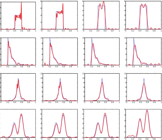
Figure 5.3 shows typical estimates of fX forn = 512 ands2n = 10 with all methods.
Note that for the sake a better visual quality, we only plot the positive part of the estimators. Our wavelet estimator is by construction a probability density function and, with that respect, is more satisfactory than the two competitors that may take
negative values. When fX is not smooth (i.e. for Uniform, Exponential and Laplace
signals is much better with our wavelet estimator. For the smooth density MixtGauss, the model selection estimator performs slightly better than the two other methods.
0 0.2 0.4 0.6 0.8 1 0 2 4 6 8 10 0 0.2 0.4 0.6 0.8 1 0 2 4 6 8 0 0.2 0.4 0.6 0.8 1 0 1 2 3 4 5 6 0 0.2 0.4 0.6 0.8 1 0 1 2 3 4 5 6 0 0.2 0.4 0.6 0.8 1 0 2 4 6 8 10 0 0.2 0.4 0.6 0.8 1 0 2 4 6 8 10 0 0.2 0.4 0.6 0.8 1 0 2 4 6 8 10 0 0.2 0.4 0.6 0.8 1 0 2 4 6 8 10 0 0.2 0.4 0.6 0.8 1 0 2 4 6 8 10 12 0 0.2 0.4 0.6 0.8 1 0 2 4 6 8 10 12 0 0.2 0.4 0.6 0.8 1 0 2 4 6 8 10 12 0 0.2 0.4 0.6 0.8 1 0 2 4 6 8 10 12 0 0.2 0.4 0.6 0.8 1 0 1 2 3 4 5 6 0 0.2 0.4 0.6 0.8 1 0 1 2 3 4 5 6 0 0.2 0.4 0.6 0.8 1 0 1 2 3 4 5 6 0 0.2 0.4 0.6 0.8 1 0 1 2 3 4 5
Figure 5.3: Typical reconstructions from a single simulation of four contaminated densities: Uniform, Exponential, Laplace, and MixtGauss. Estimators are: non-TI wavelet thresholding (1st column), TI wavelet thresholding (2nd column), model selection (3rd column) and cosine series (4th column). The scale j1 considered in the wavelet estimators depend on the true
density: j1 = 3 for the Laplace density, and j1 = 4 for the three other densities. In all figures,
the dotted lines is the true density and the solid lines is the estimator (n=512 ands2n=10). By inspecting the first column in Figure 5.3 we see that the wavelet estimator is affected by pseudo-Gibbs phenomena. A possible remedy to this defect is to use a translation invariant (TI) procedure such as the one suggested by Donoho and Raimondo (2004) for Meyer wavelet-based deconvolution in a regression setting. In the second column of Figure 5.3 we display the TI version of the wavelet estimators plotted in the first column. Observe that TI estimators remarkably exhibit very small oscillations while preserving a good reconstruction of the singularities of the
non-smooth densities. Note that non-smoother estimates can also be obtained by using a soft thresholding rule.
We also give the result of some Monte Carlo exercises. Here, we consider the
four test densities for various sample sizes (n = 128, 512) and various levels of
noise (s2n = 100, 10, 3). Note that s2n = 100 corresponds to a noise with a very
small variance, and therefore that model is very close to the direct density estimation
problem with uncontaminated data. For each combination of these factors, we
simulate 100 independent samples of sizen and compute the integrated square error
(ISE),∑mi=1(fˆn(ti)− f(ti))2/m, whereti = i/m, i = 0, . . . ,m−1. The ISE is computed
in Table 1 for m = n (this choice is not critical and the conclusions below remain for
m 6=n). Note also that our choice of computing the ISE instead of the Kullback Leibler
divergence was guided by the fact that the competing methods do not always provide a stricly positive estimator of the unknown density.
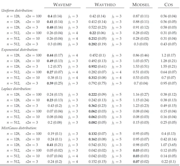
Table 1 shows the mean and the variance of the integrated square error (ISE) for various estimators. For wavelet deconvolution, we report the results of the two
thresholdings: wavtheo is based on τj whereas wavemp is constructed with ˜τj. We
also indicate the level j1 leading to the smallest empirical mean of ISE’s over the 100
simulations. As it can be observed from Table 1, the new estimator outperforms the
competitors for all type of non-smooth densities fX. It confirms the superiority of
wavelet-based positive estimators over those based on Fourier decompositions for the reconstruction of signals with local singularities. The wavelet thresholding with the
scale parameter τj = 22jν gives generally better results. When the true density is a
mixture of Gaussian random variables, the wavelet approach is better for n = 128
while the model selection procedure is slightly better than wavelet thresholding for
n = 512. Note that the fine level j1 that gives the best results is generally quite low
(although it is larger than the theoretically optimal level j1∗). For some combinations
of the parameters of the Monte Carlo simulation, the choices j1 = 3, 4 yield to the best
results. This observation is consistent with the condition of Theorem 4.2 that suggests
a smaller j1 for ill-posed inverse problems than in the direct case. It also confirms that
introducing higher level of resolution does not necessarily improve the quality of the estimator.
WAVEMP WAVTHEO MODSEL COS Uniform distribution: n=128, s2n=100 0.4(0.14) j1=3 0.42 (0.14) j1=3 0.87 (0.11) 0.56 (0.04) n=128, s2n=10 0.41(0.14) j1=3 0.412 (0.14) j1=3 0.88 (0.11) 0.56 (0.05) n=128, s2n=3 0.48(0.16) j1=3 0.522 (0.23) j1=3 0.91 (0.12) 0.58 (0.03) n=512, s2n=100 0.26 (0.04) j1=4 0.22(0.06) j1=3 0.28 (0.02) 0.31 (0.05) n=512, s2n=10 0.26 (0.04) j1=4 0.212(0.05) j1=3 0.28 (0.02) 0.31 (0.04) n=512, s2n=3 0.3 (0.08) j1=3 0.282(0.19) j1=3 0.3 (0.03) 0.43 (0.07) Exponential distribution: n=128, s2n=100 0.44(0.17) j1=4 0.452 (0.1) j1=3 0.86 (0.46) 1.2 (0.17) n=128, s2n=10 0.49(0.13) j1=3 0.492 (0.13) j1=3 1.03 (0.57) 1.28 (0.21) n=128, s2n=3 1.2 (0.37) j1=3 0.952(0.61) j1=3 1.53 (0.51) 1.55 (0.21) n=512, s2n=100 0.27(0.07) j1=4 0.282 (0.07) j1=4 0.51 (0.03) 0.64 (0.07) n=512, s2n=10 0.38 (0.1) j1=4 0.312(0.08) j1=4 0.53 (0.03) 0.7 (0.07) n=512, s2n=3 0.59(0.25) j1=3 0.792 (0.75) j1=3 0.7 (0.04) 0.95 (0.07) Laplace distribution: n=128, s2n=100 0.24 (0.13) j1=3 0.222(0.09) j1=5 1.16 (0.27) 0.38 (0.12) n=128, s2n=10 0.23(0.13) j1=3 0.242 (0.13) j1=5 1.15 (0.24) 0.38 (0.13) n=128, s2n=3 0.43 (0.2) j1=3 0.362(0.23) j1=3 1.23 (0.23) 0.49 (0.15) n=512, s2n=100 0.07 (0.04) j1=3 0.062(0.03) j1=3 0.08 (0.04) 0.15 (0.04) n=512, s2n=10 0.08 (0.04) j1=3 0.062(0.03) j1=3 0.08 (0.03) 0.16 (0.04) n=512, s2n=3 0.2 (0.08) j1=3 0.082(0.05) j1=3 0.15 (0.03) 0.25 (0.05) MixtGauss distribution: n=128, s2n=100 0.19 (0.1) j1=3 0.132(0.07) j1=5 0.95 (0.05) 0.4 (0.13) n=128, s2n=10 0.24 (0.1) j1=3 0.162(0.08) j1=5 0.95 (0.07) 0.42 (0.14) n=128, s2n=3 0.41(0.21) j1=3 0.542 (0.31) j1=3 0.98 (0.07) 1.07 (3.65) n=512, s2n=100 0.05 (0.02) j1=3 0.042 (0.02) j1=3 0.03(0.01) 0.12 (0.05) n=512, s2n=10 0.07 (0.04) j1=4 0.042 (0.02) j1=3 0.03(0.01) 0.14 (0.05) n=512, s2n=3 0.24 (0.2) j1=4 0.152 (0.15) j1=3 0.07(0.02) 0.22 (0.1)
Table 1: Empirical mean and standard deviation (in brackets) of the ISE over M = 100 repetitions for each method and some combination of the factors n ands2n. In the wavelet-based methods, only the level j1 leading to the smallest empirical mean is reported. The
smallest ISE over lines is bolded.
6
Conclusion and perspectives
Compared to the some recent deconvolution methods, the above results demonstrate the significant improvement given by the nonlinear wavelet thresholding estimator by information projection: The estimator is showed to have an optimal rate of convergence over a reasonable class of functions and a thorough empirical study proved the satisfactory behaviour of the estimator on finite sample.
The empirical study also showed that the theoretical optimal level j∗1 = (2ν+
1)−1log2(n) is usually too small for the practice. This phenomenon is not surprising
and has also been noticed e.g. in Johnstone et al. (2004). Future research could be
devoted to a tighter, non asymptotic control for the risk of estimation (e.g. via oracle-type inequalities). This would be most useful in order to develop an automatic,
data-driven selection of j1. Similarly, a specific work onτj,k is also needed. A possible way
to address the problem is to extend to our setting the corresponding work provided by (Juditsky and Lambert-Lacroix, 2004) in the standard regression model.
7
Appendix
We start by a technical lemma used in the proof of the main results. In what follows,C
denotes a generic constant whose value may change from line to line.
Lemma 7.1 Assume that the Fourier coefficients of fY are such that |flY| 6 C|l|−u with u >1. Then, E(αˆ n,λ−αλ)2 6 C n2 2|λ|ν whereαˆn,λ =∑l ψλl fǫ l 1 n ∑nj=1e−2πilYj andαλ =∑l ψλl fǫ l f Y l . PROOF: For|λ| = j, letCj ={ℓ : ψλ
ℓ 6=0}. Since the Meyer wavelets are band-limited,
Cj = {ℓ : 2j 6 |l| 6 2j+r} for some fixed r > 0. To simplify the notation, we shall
assume that Cj = {ℓ : 2j 6 l 6 2j+r} noticing that all the bounds below also hold
for negative values ofℓ. Then, using Assumption 1.1, we use|ψλ
ℓ| 6 C2−|λ|/2and the
independence of theYi’s in order to write
E(αˆn ,λ−αλ)2 6 C n2 2|λ|ν2−|λ| 2 |λ|+r
∑
ℓ,ℓ′=2|λ| Ee−2πi(ℓ−ℓ′)Y1 6 C n2 2|λ|ν+C n2 2|λ|ν2−|λ|∑
ℓ6=ℓ′ fℓY−ℓ′As |fℓY| 6 C|ℓ|−u with u > 1, the double sum ∑ℓ6=ℓ′ fℓY−ℓ′ in the equation above is
bounded which yields the result.
Proof of the main theorems. The proof of the two main theorems is based on a decomposition of the relative entropy between the true and the estimated density function into the sum of two terms which correspond to approximation error and
estimation error (bias and variance in a familiar mean squared error analysis). This decomposition is given by ∆(fX; fj, ˆθ n) = ∆(f X; f j,θ∗j) +∆(fj,θ∗j; fj, ˆθn) (7.1)
where fj,θ∗j denotes the closest function of Ej to the true density fX for the
Kullback-Leibler divergence. This identity comes from the Pythagorean Theorem derived
in Csisz´ar (1975). It allows in particular to write the risk E∆(fX; f
j(n), ˆθn) as the
sum of an approximation error term ∆(fX; f
j(n),θ∗j(n)) and an estimation error term
E∆(fj(n),θ∗
j(n); fj(n), ˆθn).
The control of the approximation error term is similar for the linear and the nonlinear estimators. Below, we only sketch the proof of the existence and uniqueness
of fj,θ∗j as this follows from the arguments in Antoniadis and Bigot (2006) and by
applying Barron and Sheu (1991, Lemma 5). To do so, note that the technical lemmas in Appendix A of Antoniadis and Bigot (2006) need to be adapted to the case of Meyer wavelets.
The control of the estimation error term differs for the linear or the nonlinear
estimators. In the linear case, it simply relates to the control of the risk Ekαˆn −α0k2
2
which is given by Lemma 7.1. In the nonlinear situation, we use some classical moment bounds (Rosenthal (1972)) and Bernstein’s inequality to control the difference between the estimated wavelet coefficients and their true values, together with the maxiset
theorem of Johnstoneet al. (2004).
For the periodised Meyer wavelet basis and under the conditions of Theorem 4.2
for s,p,q,ν, τj,n, j1, this maxiset theorem says that an estimator of the form ˆfh =
∑j1
j=j0−1∑|λ|=jδ
h
τj,n(βˆλ)ψλ satisfies the asymptotic rate of convergeEkfˆh− fk2L2([0,1]) 6
C(lognn)2s/(2s+2ν+1) provided that 2j1(n) = O
(logn(n))1/(2ν+1), and if for η large
enough, there exists two constantC1andC2such that for alln∈ N∗ and|λ|= j
E|βˆλ−βλ|4 6 C1τ 4 j n2, (7.2) P |βˆλ−βλ|>ητj q (logn)/n 6 C2(logn n ) 2, (7.3)
where the βλ’s are the wavelet coefficients of f (see Johnstoneet al. (2004) for further
Proof of Theorem 4.1. We first consider the control of the approximation term. By arguing as in Barron and Sheu (1991) and Antoniadis and Bigot (2006), and under the
assumptions of Theorem 4.1 , one can prove that for n sufficiently large, there exists
some θ∗j(n) such that hfX,ψλi = hfj(n),θ∗j(n),ψλi for all |λ| < j(n), which satisfies for
2−j(n) =O(n−1/(2s+2ν+1))
∆(fX; fj(n),θ∗
j(n)) = O
2−2j(n)s=On−2s/(2s+2ν+1). (7.4)
We now turn to the estimation error term. For all |λ| < j(n), define α0,λ =
hfX,ψλi = hfj,θ∗j,ψλi and let ˆαn,λ = ∑l(ψλl /flǫ)∑nj=1exp(−2πilYj)/n. To prove the
existence of a vector ˆθn ∈ R2
j(n)
such that hfj, ˆθ
n,ψλi = αˆn,λ, for all|λ| < j(n), we
need to control the term kαˆn −α0k22 = ∑|λ|<j(n)(αˆn,λ −α0,λ)2 and then to apply
Barron and Sheu (1991, Lemma 5). Given our assumption on fX and fǫ we have that
|flY| 6 C|l|−(s+ν) with s+ν > 1, and we can therefore apply Lemma 7.1 to obtain
thatEkαˆn −α0k2
2 6 C2j(n)(2ν+1)/n Then, under the assumptions of Theorem 4.1, and
arguing as in Antoniadis and Bigot (2006) and by applying Barron and Sheu (1991,
Lemma 5), we have that fornsufficiently large, ˆθn exists and is such that
E∆(fj(n),θ∗
j(n); fj(n), ˆθn)
=On2j(n)(2ν+1)=On−2s/(2s+2ν+1), (7.5) for 2−j(n) = On−1/(2s+2ν+1)). The result of the theorem now follows from the control
of the approximation and estimation error terms, using the identity (7.1).
Proof of Theorem 4.2.By proceeding as in Antoniadis and Bigot (2006), one can show
that for n sufficiently large, there exists someθ∗j
1(n) such that for 1 6 p 6 2 and s
>
1/2+1/p, it holds∆(fX; f j1(n),θ∗j
1(n)
) = O(2−2j1(n)(s−1/2−1/p)), where we have used the
notations from the proof of Theorem 4.1. Then, since 2j1(n) = O({log(n)/n}1/(2ν+1)),
we can write ∆(fX; fj
1(n),θ∗j
1(n)
) = O({log(n)/n}2(s−1/2−1/p)/(2ν+1)). Since s > (2ν+
1)(1/p+1/2)by assumption, we therefore obtains−1/2−1/p >2sν/(2ν+1)and
the condition s > 1/2+1/4ν finally implies that 2sν/(2ν+1)2 > 2s/(2s+2ν+1)
which yields the near-optimal order of convergence for the approximation term ∆(fX; fj1(n),θ∗
j1(n)) =O({log(n)/n}
2s/(2s+2ν+1)).
We can now consider the estimation error term. Define ˆαn,λ andαλ as in the proof
of Theorem 4.1. Define Ekδh τj,n(αˆn)−α0k 2 2 = ∑j0−16|λ|<j1(n)E(δ h τj,n(αˆn,λ)−αλ) 2 with
maxiset theorem of Johnstoneet al. (2004). Given our conditions imposed onp,q,s,ν,j1
andτj,n it remains to check (7.2) and (7.3) with ˆβλ =αˆn,λ andβλ =αλ.
Before we recall a useful result for moment bounds of iid variables (Rosenthal, 1972): IfZ1, . . . ,Zn are iid random variables such thatEZj =0,EZ2j 6σ2, then ifm > 2, there exists a positivecm such thatE|∑nj=1Zj/n|m 6cm(σm/nm/2+E|Z1|m/nm−1).
Recall that ˆαn,λ−αλ =n−1∑nj=1(∑l(e−2πilYj− flY)ψlλ/flǫ). For|λ|= j, letCj ={l :
ψλl 6= 0}. Since the Meyer wavelets are band-limited, Cj = {l : 2j 6 |l| 6 2j+r}
for some fixed r > 0. To simplify the notation, we shall assume that Cj = {l :
2j 6 l 6 2j+r} noticing that all the bounds below also hold for negative values of
ℓ. Hence, we have that ˆαn,λ−αλ = 1
n ∑nj=1Zj, where theZj’s are iid variables such that
Zj =∑2|λ|+r l=2|λ| ψlλ fǫ l e−2πilYj− fY l .
First notice that EZj = 0. In order to apply Rosenthal’s inequality, it remains
to derive a bound for E|Zj|2 and E|Zj|4. Denote by gλ the function gλ(x) =
∑2|λ|+r
l=2|λ|(ψλl/flǫ)exp(−2πilx), and observe that the inequality
E|Z j|2 =E|gλ(Yj)−αλ|2 6C Z |gλ(y)|2dy+|αλ|2 (7.6) holds. Then by Parseval equality, one has that
Z |gλ(y)|2dy = 2|λ|+r
∑
l=2|λ| |ψlλ/flǫ|2 6C2|λ|2ν, (7.7)where we have used the fact thatα2λ = (R1
0 f(x)ψλ(x)dx)2 6
R1
0 f(x)2dx
R1
0 ψλ(x)2dxis
thus bounded by some constantC for any λ, that∑2|λ|+r
l=2|λ| ψλ l 2 = 1 , and Assumption
1.1. Inserting (7.6) into (7.7) yields E|Zj|2 = E|gλ(Yj) −αλ|2 6 C2|λ|2ν. Using the inequality(a+b)4 68(a4+b4)that is valid for any reala,b, we get
E|Z j|4 =E|gλ(Yj)−αλ|4 6C Z |gλ(y)|4dy+|αλ|4 . (7.8)
Then, observe that R
|gλ(y)|4dy 6 |gλ|2∞
R
|gλ(y)|2dy 6 C2|λ|(2ν+1)2|λ|2ν, where we
have used |gλ|∞ 6 ∑2|
λ|+r
l=2|λ||ψλl /flǫ| 6 C2|λ|ν2|λ|/2 which comes from the fact |ψlλ| 6
C2−|λ|/2and from Assumption 1.1. With (7.8) and using the fact that|αλ|46 Cfinally
leads toE|Zj|4 6C2|λ|(4ν+1).
Now, if we apply Rosenthal’s inequality with m = 4 and for |λ| = j we obtain
E|αˆ
τj2 = 22jν and given that for j 6 j1(n), one has that 2j
n 6 C, we finally obtain that
24jν/n2 6 Cτ4
j/n2 and 2j(4ν+1)/n3 6Cτj4/n. It leads toE|αˆn,λ−αλ|4 6Cτj4/n2, holds
true. This development proves that ˆαn,λ−αλ satisfies the condition (7.2).
Now, recall the standard Bernstein’s inequality: let Z1, . . . ,Zn be i.i.d. random
variables withEZj =0,EZ2
j 6σ2, |Zj|6kZk∞ <+∞, then for anyλ>0
P 1 n n
∑
j=1 Zj >λ ! 62 exp − nλ2 2(σ2+kZk∞λ/3) .Now, let us apply Bernstein’s inequality with theZj’s as defined previously. From (7),
we have thatEZ2
j 6C2|λ|2νand arguing as previously, one has that|Zj|6C2|λ|(ν+1/2).
Therefore, the following bound holds for|λ| =j(for some constantC1andC2)
P |αˆn,λ−αλ| >ητj q (logn)/n 6 2 exp − η2log(n) 2(C1+C22j/2η(logn/n)1/2) , 6 2 exp−Cη2log(n).
Hence, forη large enough one has that for alln >1P(|αˆ
n,λ−αλ|>ητj
p
log(n)/n) 6 C{log(n)/n}2, which proves that ˆα
n,λ−αλsatisfies the condition (7.3).
Hence, from the maxiset theorem in Johnstone et al. (2004), we finally derive the
following upper bound : Ekδh
τj,n(αˆn)−α0k
2
2 =O({log(n)/n}2s/(2s+2ν+1)).
In order to prove the existence of the projection estimate fh
j1(n), ˆθn we proceed as in
Antoniadis and Bigot (2006). Under the assumptions of Theorem 4.1 and by applying
Barron and Sheu (1991, Lemma 5), one can show that for n sufficiently large, fh
j(n), ˆθn
exists and is such thatE(∆(fj(n),θ∗
j(n); f
h
j(n), ˆθn)) = O({log(n)/n}
2s/(2s+2ν+1)). The result
of the theorem now follows from the control of the approximation and estimation error
terms, using the identity (7.1).
References
Antoniadis, A. and Bigot, J. (2006). Poisson inverse problems. Ann. Statist., 34,
2132-2158.
Barron, A. R. and Sheu, C. H. (1991). Approximation of density functions by sequences
of exponential families. Ann. Statist.,19, 1347–1369.
Buckheit, J., Chen, S., Donoho, D. and Johnstone, I. (1995). Wavelab reference manual
Carroll, R. and Hall, P. (1988). Optimal rates of convergence for deconvolving a density.
J. Amer. Statist. Assoc.,83, 1184–1186.
Comte, F., Rozenholc, Y. and Taupin, M.-L. (2006). Penalized contrast estimator for
density deconvolution. Canad. J. Statist.,34, XXX.
Comte, F., Rozenholc, Y. and Taupin, M.-L. (2007). Finite sample penalization in
adaptive density deconvolution. J. Stat. Comput. Simul.,7, 977–1000.
Csisz´ar, I. (1975). I-divergence geometry of probability distributions and minimization
problems. Ann. Probab.,3, 146–158.
De Canditiis, D. and Pensky, M. (2006). Simultaneous wavelet deconvolution in
periodic setting. Scand. J. Statist.,33, 293–306.
Donoho, D. L. and Raimondo, M. (2004). Translation invariant deconvolution in a
periodic setting. Int. J. Wavelets Multiresolut. Inf. Process.,4, 415–431.
Fan, J. (1991). On the optimal rate of convergence for nonparametric deconvolution
problems. Ann. Statist.,19, 1257–1272.
Fan, J. and Koo, J.-Y. (2002). Wavelet deconvolution. IEEE Trans. Inform. Theory, 48,
734–747.
Hall, P. and Qiu, P. (2005). Discrete-transform approach to deconvolution problems.
Biometrika,92, 135–148.
Johannes, J., Van Bellegem, S. and Vanhems, A. (2007). A unified approach to solve
ill-posed inverse problems in econometrics. (www.stat.ucl.ac.be/ISpub)
Johnstone, I., Kerkyacharian, G., Picard, D. and Raimondo, M. (2004). Wavelet
deconvolution in a periodic setting. J. Roy. Statist. Soc. Ser. B,66, 547–573.
Juditsky, A. and Lambert-Lacroix, S. (2004). On minimax density estimation on R.
Bernoulli,10, 187–220.
Kolaczyk, E. (1994). Wavelet methods for the inversion of certain homogeneous linear
operators in the presence of noisy data. Ph.d. thesis, Stanford University.
Koo, J.-Y. (1999). Logspline deconvolution in Besov space. Scand. J. Statist.,26, 73–86.
Koo, J.-Y. and Chung, H.-Y. (1998). Log-density estimation in linear inverse problems.
Ann. Statist.,26, 335–362.
Koo, J.-Y. and Kim, W.-C. (1996). Wavelet density estimation by approximation of
log-densities. Statistics and Probability Letters,26(3), 271-278.
Mallat, S. (1998). A wavelet tour of signal processing. New York: Academic Press.
Pensky, M. and Vidakovic, B. (1999). Adaptive wavelet estimator for nonparametric
density deconvolution. Ann. Statist.,27, 2033–2053.
Rosenthal, H. P. (1972). On the span in Lp of sequences of independent random