Empirical likelihood estimators for the error distribution in nonparametric regression models

econstor

www.econstor.eu

The Open Access Publication Server of the ZBW – Leibniz Information Centre for Economics

Nutzungsbedingungen:

Die ZBW räumt Ihnen als Nutzerin/Nutzer das unentgeltliche, räumlich unbeschränkte und zeitlich auf die Dauer des Schutzrechts beschränkte einfache Recht ein, das ausgewählte Werk im Rahmen der unter

→ http://www.econstor.eu/dspace/Nutzungsbedingungen nachzulesenden vollständigen Nutzungsbedingungen zu vervielfältigen, mit denen die Nutzerin/der Nutzer sich durch die erste Nutzung einverstanden erklärt.

Terms of use:

The ZBW grants you, the user, the non-exclusive right to use the selected work free of charge, territorially unrestricted and within the time limit of the term of the property rights according to the terms specified at

→ http://www.econstor.eu/dspace/Nutzungsbedingungen By the first use of the selected work the user agrees and declares to comply with these terms of use.

zbw

Kiwitt, Sebastian; Nagel, Eva-Renate; Neumeyer, Natalie

Working Paper

Empirical likelihood estimators for the error

distribution in nonparametric regression models

Technical Report / Universität Dortmund, SFB 475 Komplexitätsreduktion in Multivariaten Datenstrukturen, No. 2005,45

Provided in cooperation with:

Technische Universität Dortmund

Suggested citation: Kiwitt, Sebastian; Nagel, Eva-Renate; Neumeyer, Natalie (2005) : Empirical likelihood estimators for the error distribution in nonparametric regression models, Technical Report / Universität Dortmund, SFB 475 Komplexitätsreduktion in Multivariaten Datenstrukturen, No. 2005,45, http://hdl.handle.net/10419/22638

Empirical likelihood estimators for the error

distribution in nonparametric regression

models

Sebastian Kiwitt, Eva-Renate Nagel and Natalie Neumeyer*

Fakult¨at f¨

ur Mathematik, Ruhr-Universit¨at Bochum

44780 Bochum, Germany

*

October 13, 2005

Abstract

The aim of this paper is to show that existing estimators for the error distribution in nonparametric regression models can be improved when additional information about the distribution is included by the empirical likelihood method. The weak convergence of the resulting new estimator to a Gaussian process is shown and the performance is investigated by comparison of asymptotic mean squared errors and by means of a simulation study. As a by-product of our proofs we obtain stochastic expansions for smooth linear estimators based on residuals from the nonparametric regression model.

Short title: Empirical likelihood for regression errors AMS Classification: 62G08, 62G05

Keywords and Phrases: empirical distribution function, empirical likelihood, error distribution, estimating function, nonparametric regression, Owen estimator

1

Introduction

Since a few decades in statistical research nonparametric regression models have been investi-gated intensively. We consider such a model,

with independent observations (X1, Y1), . . . ,(Xn, Yn) and centered, unobserved, independent

and identically distributed errors ε1, . . . , εn (independent from the design points X1, . . . , Xn).

In the last decades research focused mainly on nonparametric estimation of the regression function m and variance σ2 _{= E[ε}2

1] and corresponding hypotheses tests. Since a few years

only there exist results on estimation of the distribution of the unobserved errors ε1, . . . , εn.

For example, consistent estimators for the regression function and error distribution can be used to evaluate prediction intervals for future observations at some point x [see Akritas and Van Keilegom (2001)]. Further the empirical distribution function of estimated errors recently turned out to be valuable for goodness-of-fit tests concerning the regression or variance function, see Van Keilegom, Gonz´alez Manteiga and S´anchez Sellero (2004) and Dette and Van Keilegom (2005), or for testing the equality of regression functions in a two–sample problem, see Pardo-Fern´andez, Van Keilegom and Gonz´alez-Manteiga (2004) and Neumeyer and Dette (2005). We denote byFnthe (not available) empirical distribution function of unobserved errors. Classical

results by Donsker (1952) show weak convergence of the empirical process √n(Fn −F) to a

Brownian bridge B with covariance structure

Cov(B(y), B(z)) = F(y_∧z)₋F(y)F(z).

(1.1)

Now, let ˆFndenote the empirical distribution function of nonparametrically estimated residuals,

i.e. ˆ Fn(y) = 1 n n X i=1 I_{εˆi ≤y}, y∈R, (1.2)

where the residuals are defined as ˆεi = Yi −mˆ(Xi), and ˆm denotes the Nadaraya–Watson

estimator for the regression function m. The asymptotic behavior of ˆFn has been investigated

by Akritas and Van Keilegom (2001) and Cheng (2002). A smooth version of ˆFnwas considered

by M¨uller, Schick and Wefelmeyer (2004c). Cheng (2004), Qin (1996), and Qin, Shi and Chai (1996) propose corresponding error density estimators. In the heteroscedastic model considered by Akritas and Van Keilegom (2001) the regression and variance function are defined as L-functionals depending on some score function J. Slight adaptations of Akritas and Van Keilegom’s (2001) arguments for a homoscedastic regression model and score function J _≡ 1 show under some regularity assumptions (that are valid under the assumptions stated in section 2 of the presented paper) that the process√n( ˆFn(·)−F(·)−b(·)) converges weakly to a Gaussian

process Gwith covariance structure

Cov(G(y), G(z)) = F(y_∧z)₋F(y)F(z) (1.3)

where f denotes the error density and the bias term is defined as b(y) = h2f(y)1 2 Z K(u)u2du Z ((mfX)00(x)−(mfX00)(x))dx. (1.4)

Here K denotes a kernel function and h a bandwidth used for the construction of the kernel estimator ˆm and fX denotes the density of the design points. We give a short derivation of

this result in appendix A. One notices that the covariance structure of the asymptotic process

G given in (1.3) differs from the covariance structure of the asymptotic process B, see (1.1). For Gaussian errors considering nonparametric residuals instead of true errors even results in a uniformly smaller asymptotic variance,

Var(G(y)) _≤ Var(B(y)) _∀y_∈R,

but the estimation is biased then. We want to investigate whether the estimation of the error distribution can further be improved in terms of mean squared error when additional information is used. Our most important example for additional information is the centeredness of the errors, i. e. E[ε1] = 0, that is required by the model but is not explicitely used in the

estimation ˆFn. Further examples for additional information are a known variance or median.

Improvements of the estimator by including additional information could be obtained by the Empirical Likelihood method that was introduced by Owen (1988, 2001) and further developed by Hall and LaScala (1990), DiCiccio, Hall and Romano (1989, 1991), DiCiccio and Romano (1989), Hall (1990), Kitamura (1997), Einmahl and McKeague (2003), among many others. Qin and Lawless (1994) and Zhang (1997) considered the problem of estimating the distribution of an (observed) iid-sample ε1, . . . , εn when auxiliary information is available in terms of

E[g(ε1)] =

Z

g(y)dF(y) = 0,

where g = (g1, . . . , gk)T :R →Rk is a known function such that E[gj2(ε1)]<∞ (j = 1, . . . , k).

This could be, for example, g(ε) = ε for the model assumption of centered errors, g(ε) = (ε, ε2_−σ2₎T _{for centered errors with a known variance σ}2 _{or g(ε) = I{ε ≤q} −} 1

2 for a priori

information about the median q. The empirical likelihood estimator for the error distribution is ˜ Fn(y) = n X i=1 piI{εi ≤y}, y∈R, (1.5)

where the weights pi ∈(0,1) are chosen such that the empirical likelihood n

Y

i=1

pi

is maximized under the constraints n X i=1 pi = 1, Z g(y)dF˜n(y) = n X i=1 pig(εi) = 0. (1.7)

Qin and Lawless (1994) and Zhang (1997) showed that in this setting the obtained empirical likelihood estimator has a uniformly smaller asymptotic variance than the empirical distribution function. For empirical likelihood and moment restrictions see also Kitamura (2001), Kitamura, Tripathi, Ahn (2004), and Bonnal and Renault (2004), among others.

The empirical likelihood method was applied in the context of estimation of the error distri-bution in linear models with fixed design and homoscedastic errors by Nagel (2002) using the additional information E[ε1] = 0, i. e. g(ε) = ε, that is available from the model. In this

context it depends on the method of parameter estimation whether the empirical likelihood method yields a smaller asymptotic variance than the empirical distribution function based on parametric residuals. A comprehensive study of the residual based empirical distribution functions in the linear model can be found in Koul (2002). Estimators for the error distribution in AR(1)-models including the centeredness assumption were considered by Genz (2004). In the presented paper we propose a residual based empirical likelihood method for the error distribution in nonparametric regression models when auxiliary information is available. We develop asymptotic expansions for the empirical likelihood estimator, Fn, in our context and

prove weak convergence of the process √n(Fn(·)−F(·)−b(·)) to a Gaussian processG, where

b denotes a bias term. We compare the resulting asymptotic mean squared error of the new estimator,

Var(G(y))

n +b

2

(y),

with the analogous term for the residual based empirical distribution function, Var(G(y))/n+

b2_{(y) defined in (1.3) and (1.4), in some examples. In the especially interesting case of g(ε) =ε}

(i. e. including the model assumption of centered errors explicitely into the estimation) we obtain asymptotically the same variances but a considerable reduction of bias.

As a by-product of our proofs we regain asymptotic expansions for smooth linear statistics 1 n n X i=1 g(ˆεi)

in a similar homoscedastic setting considered by M¨uller, Schick and Wefelmeyer (2004a) and prove analogous results for heteroscedastic models.

The paper is organized as follows. In section 2 we describe our (homoscedastic) model and ex-plain regularity assumptions needed to obtain the main asymptotic results presented in section

3. In section 4 we consider the analogous procedures in a heteroscedastic setting. In section 5 some examples are illustrated in order to discuss the results and in section 6 a simulation study is presented. The proofs are deferred to an appendix.

2

Model and assumptions

We first consider a nonparametric homoscedastic regression model with independent observa-tions

Yi = m(Xi) +εi, i= 1, . . . , n,

(2.1)

under the following assumptions.

(M1) The univariate design pointsX1, . . . , Xnare independent and identically distributed with

distribution function FX on compact support, say [0,1]. FX has a twice continuously

differentiable density fX, such that infx∈[0,1]fX(x) > 0. The regression function m is

twice continuously differentiable in (0,1) with bounded derivatives.

(M2) The errors ε1, . . . , εn are independent and identically distributed with distribution

func-tion F. They are centered, E[ε1] = 0, with variance σ2 = Var(ε1)∈(0,∞), and

indepen-dent from the design points. F is continuously differentiable with bounded, everywhere positive density f.

(M3) There exist constants γ, C and β >0 such that for allz _∈R with _|z_{| ≤}γ

|F(y+z)₋F(y)₋zf(y)_{| ≤} C_|z_|1+β.

Note that assumption (M3) is satisfied with β = 1 under the stronger assumption that f is continuously differentiable with sup_y∈R|f0_(y)|<∞.

In order to estimate the distribution F of the unobserved errors, one builds nonparametric residuals

ˆ

εi = Yi−mˆ(Xi), i= 1, . . . , n,

where ˆm(x) denotes the Nadaraya-Watson estimator [Nadaraya (1964), Watson (1964)] for

m(x), that is ˆ m(x) = 1 n n X i=1 1 hK X_i−x h Yi 1 ˆ fX(x) (2.2)

with the kernel density estimator for fX(x), ˆ fX(x) = 1 n n X i=1 1 hK X_i−x h . (2.3)

For the kernel estimators we need the following assumptions.

(K) Let K denote a symmetric density with compact support and R

uK(u)du= 0.

(H) Leth=hn be a sequence of bandwidths such thatnh4 =O(1),nh3+2α(log(h−1))−1 → ∞

(for some α > 0) and nβ_h1+β_(log(h−1₎₎−1−β _{→ ∞ (where β is defined in assumption}

(M3)) for n _{→ ∞}.

Note that the last bandwidth condition can be omitted when 1+_ββ _≤ 3 + 2α. This is always valid for β _≥ 1₂. The constant α has only relevance in the technics of the proof and can be chosen arbitrarily small.

We denote by ˆFn the empirical distribution function based on residuals ˆε1, . . . ,εˆn defined in

(1.2). Assumptions (M1), (M2), (M3), (K) and (H) were already imposed by Akritas and Van Keilegom (2001) to show weak convergence of the residual based empirical process, √n( ˆFn−

F ₋b) [where the biasb is defined in (1.4)].

We further assume that additional information about the error distribution is available. This auxiliary information is given in terms of assumption (A).

(A) E[g(ε1)] =

R

g(y)f(y)dy= 0, where g = (g1, . . . , gk)T :R→Rk is a known function such

that E[g2

j(ε1)]<∞ for j = 1, . . . , k.

Example 2.1 The most important example to consider is g(ε) = ε because the centeredness of the errors is a given model assumption. Further a priori information, for instance, of a zero median can be described by the function g(ε) = I_{ε _≤ 0_{} −}1/2. When can be assumed, for example, that the variance is known and the third moment is zero one would define g(ε) = (ε, ε2_−σ2_{, ε}3₎T_.

Throughout the paper the following assumptions on the functiong are only assumed to be valid when stated explicitely.

(G1) We assume thatgj is continuously differentiable and there exist constants γ, C andβ >0

such that Z gj(y+z)−gj(y)−zg0j(y) f(y)dy ≤ C|z| 1+β

for all z _∈R with _|z_{| ≤}γ, j = 1, . . . , k. Moreover, let E[_|g0

[Without restriction we use the same constants γ, C and β as in assumption (M3).] (G2) There exist constants δ, C such that for some positive κ <2(1 +α)

Eh sup z,z˜∈R:|z|≤δ, |˜z|≤δ,|z−˜z|≤ξ (gj(ε1+z)−gj(ε1+ ˜z))2 i1/2 ≤ Cξ1/κ

(where α is defined in assumption (H)), j = 1, . . . , k.

Note that (G2) is, for example, satisfied for κ = 1 by Taylor’s expansion when gj is

continu-ously differentiable and E[sup_{z∈R:|z|≤δ}(g0

j(ε1+z))2]<∞(j = 1, . . . , k). Thenκ = 1<2(1 +α)

is always valid (α > 0). The smoothness assumptions (G1) and (G2) are similar to the as-sumptions imposed by M¨uller, Schick and Wefelmeyer (2004a, Assumption 1, p. 79, and 2004b, Assumption B1, p. 536) to obtain asymptotic results about smooth linear estimators based on nonparametric residuals, compare the discussion of the assumptions given there [M¨uller, Schick and Wefelmeyer (2004a, section 3)]. Note also that either with assumption (G2) or for the indicator function g(ε) =I_{ε_≤a_{} −}b it follows

∃δ >0 such that Eh sup

y∈R:|y|≤δ

(gj(ε1+y)−gj(ε1))2

i

<_{∞ ∀}j = 1, . . . , k

(2.4)

and this condition will be used repeatedly during the proof.

Example 2.2 Functions g(ε) = εk_{−c corresponding to moment assumptions fulfill}

assump-tions (G1) and (G2) when E[ε2k

1 ] < ∞. The same is valid for polynomials, for example,

g(ε) =ε4_−cε2_{, to account for a relation between second and fourth moment.}

Remark 2.3 Assumptions (G1) and (G2) are mainly imposed to obtain stochastic expansions of _n1 Pn

i=1g(ˆεi). In addition to smooth functions g satisfying (G1) and (G2) or indicator

func-tions g(ε) = I_{ε _≤ a_{} −} b the theory can be developed for every function g, such that an expansion 1_nPn i=1g(ˆεi) = 1 n Pn i=1(g(εi) +h(εi)) +oP( 1 √

n) is valid with some weak assumptions

on the function h (compare Lemma B.1 (ii), (iii) in the appendix).

We further need the following assumptions to assure a unique solution in the maximization of the empirical likelihood.

(S1) We assume that min1≤i≤ngj(ˆεi)<0<max1≤i≤ngj(ˆεi) for all j = 1, . . . , k.

(S2) We assume that Σ = E[g(ε1)g(ε1)T] andPn_i=1g(ˆεi)g(ˆεi)T are positive definite.

Note that assumption (S1) is valid in probability for an increasing sample size because of assumption (A) when the residuals ˆεi are replaced by the true errors εi. Further, the first

assumption of (S2) with Lemma B.1 (v) (in the appendix) implies the second assumption of (S2) for increasing sample size, in probability.

3

Main asymptotic results

The motivation of the empirical likelihood method is as explained in the introduction [compare (1.5)–(1.7)]. The estimator for the error distribution is

Fn(y) = n

X

i=1

piI{εˆi ≤y},

where the weights pi ∈(0,1) are chosen such that Qn_i=1pi is maximized under the constraints n X i=1 pi = 1, n X i=1 pig(ˆεi) = 0.

Analogously to Qin and Lawless (1994) we obtain the estimator

Fn(y) = 1 n n X i=1 1 1 + ˆηT ng(ˆεi) I_{εˆi ≤y}, (3.1)

where ˆηn is defined as solution of the equation n X i=1 g(ˆεi) 1 + ˆηT ng(ˆεi) = 0 (3.2)

while for all i = 1, . . . , n it holds that 1 + ˆηT

ng(ˆεi) > 1_n. The following two propositions give

stochastic expansions for the solution ˆηn as well as for the distribution estimatorFn.

Proposition 3.1 Under model (2.1) and assumptions (M1), (M2), (M3), (K), (H), (A), (S1), (S2) and with either g(ε) = I_{ε_≤a_{} −}b or g satisfying (G1), (G2) we have the expansion

ˆ ηn = Σ−1 1 n n X i=1 g(ˆεi) +oP( 1 √ n).

Proposition 3.2 Under model (2.1) and assumptions (M1), (M2), (M3), (K), (H), (A), (S1), (S2) and with either g(ε) = I_{ε _≤ a_{} −}b or g satisfying (G1), (G2) we have uniformly with respect to y_∈R,

Fn(y) = ˆFn(y)−U(y)Tηˆn+oP(

1 √

n),

where Fˆn denotes the residual based empirical distribution function defined in (1.2) andU(y) =

E[g(ε1)I{ε1 ≤y}].

We state our main results for two different cases of additional information in the Theorems 3.3 and 3.7, namely smooth functions g that satisfy assumptions (G1) and (G2) resp. indicator functions that give quantile informations.

Theorem 3.3 Under model (2.1) and assumptions (M1), (M2), (M3), (K), (H), (A), (G1), (G2), (S1) and (S2) we have uniformly in y_∈R the expansion

Fn(y) =b(y) + 1 n n X i=1 h I_{εi ≤y}+f(y)εi−U(y)TΣ−1(g(εi)−E[g0(ε1)]εi) i +oP( 1 √ n)

where the bias term is defined as b(y) =h2_{B(f(y) +U(y)}T_Σ−1_E[g0_(ε

1)]) with B = 1 2 Z K(u)u2du Z ((mfX)00(x)−mfX00(x))dx,

and U(y), Σ are defined in Proposition 3.2 and assumption (S2), respectively. The process

√

n(Fn(·)−F(·)−b(·)) converges weakly to a centered Gaussian process G with covariance

structure Cov(G(y), G(z)) = F(y_∧z)₋F(y)F(z) +f(y)f(z)σ2 +f(y)E[ε1I{ε1 ≤z}] +f(z)E[ε1I{ε1 ≤y}] +U(y)TΣ−1Σ₋E[g0(ε1)]E[ε1gT(ε1)] −E[ε1g(ε1)]E[g0(ε1)]T +E[g0(ε1)]σ2E[g0(ε1)]T Σ−1_U(z) −UT(y)Σ−1U(z)₋E[g0(ε1)]E[ε1I{ε1 ≤z}] −UT(z)Σ−1U(y)₋E[g0(ε1)]E[ε1I{ε1 ≤y}] −f(z)U(y)T +f(y)U(z)TΣ−1E[ε1g(ε1)]−E[g0(ε1)]σ2 .

The proof of Theorem 3.3 is given in appendix C. It is not true that for all distributions uniformly in ythe asymptotic variance of the empirical likelihood estimator is smaller than the asymptotic variance of the residual based empirical distribution function as it is the case for an observed iid-sample ε1, . . . , εn. Different functionsg and underlying distributionsF have to

be investigated. Also, bias and variance have to be taken into account simultaneously for the comparison as we will do in the discussion of the asymptotic results in section 5.

Remark 3.4 Note that under a stronger bandwidth condition nh4 _{=o(1) the bias term b(y)}

in Theorem 3.3 is negligible. It can be seen from the expansion stated in the Theorem that incorporating the auxiliary information about the error distribution does not lead to a smaller asymptotic variance in the case g(ε) = E[g0_{(ε)]ε because then F}

n = ˆFn +oP(n−1/2). Then,

using the auxiliary information that the errors are centered, that is g(ε) =ε, does not change the variance asymptotically. A heuristic explanation for this phenomenon was given by M¨uller, Schick and Wefelmeyer (2004a) in the similar context of linear smooth residual based estimators

by the statement that the mean zero information is already used for estimating ˆεi. However,

the bias terms of orderh2 _{should also be taken into account under the less restrictive bandwidth}

condition nh4 _{=O(1). The bias changes fromb(y) defined in (1.4) tob(y) when using empirical}

likelihood and the latter term can be considerably smaller as will be discussed in section 5. Corollary 3.5 Under the assumptions of Theorem 3.3 we have Var(G(y)) = Var(G(y))for all

y _∈R if and only if g(ε) =cε for some c_∈R.

Remark 3.6 As a by-product of the proof of Theorem 3.3 we obtain the following asymptotic expansion for smooth linear estimators based on nonparametric residuals,

1 n n X i=1 g(ˆεi) = 1 n n X i=1 (g(εi)−E[g0(ε1)]εi)−h2E[g0(ε1)]B+oP( 1 √ n)

where B is defined in Theorem 3.3 [compare Lemma B.1 (ii) in the appendix]. This completes results given by M¨uller, Schick and Wefelmeyer (2004a, 2004b), who considered more restrictive bandwidth conditions to neglect the bias and used a leave-one-out local polynomial estimator for the regression function.

Next we state our asymptotic results for indicator functions g that include additional informa-tion about quantiles. The proof of Theorem 3.7 is given in appendix C.

Theorem 3.7 Under model (2.1) and assumptions (M1), (M2), (M3), (K), (H), (A), (S1) and (S2) where g(ε) = I_{ε _≤ a_{} −}b for some constants a and b = F(a) _{6∈ {}0,1_} (k = 1) we have uniformly in y _∈R the expansion

Fn(y) =b(y) + 1 n n X i=1 h I_{εi ≤y}+f(y)εi−U(y) 1 b(1₋b)(I{εi ≤a} −b+f(a)εi) i +oP( 1 √ n)

where the bias term is b(y) = h2_{B(f(y) − Σ}−1_{U(y)f(a)) with B defined in Theorem 3.3.}

The process √n(Fn(·)−F(·)−b(·)) converges weakly to a centered Gaussian process G with

covariance structure Cov(G(y), G(z)) = F(y_∧z)₋F(y)F(z) +f(y)f(z)σ2 +f(y)E[ε1I{ε1 ≤z}] +f(z)E[ε1I{ε1 ≤y}] +(b(1₋b))−2U(z)U(y)b(1₋b) + 2f(a)E[ε1I{ε1 ≤a}] +f2(a)σ2 −(b(1₋b))−1U(z)F(a_∧y)₋bF(y) +f(a)E[ε1I{ε1≤y}] −(b(1₋b))−1U(y)F(a_∧z)₋bF(z) +f(a)E[ε1I{ε1 ≤z} −(b(1₋b))−1f(z)U(y) +f(y)U(z)E[ε1I{ε1 ≤a}] +f(a)σ2 .

Remark 3.8 For the ease of presentation we stated results for k-dimensional smooth functions

g in Theorem 3.3 and for one dimensional indicator functions in Theorem 3.7. Results can straightforwardly be generalized to k-dimensional vectors g of indicator functions for including information about k quantiles, or vectors with some smooth components and some indicator function components. Further, results can be generalized for all information functions g with expansions similar to those given in Lemma B.1 (ii) or (iii).

4

The heteroscedastic case

In this section we consider a nonparametric heteroscedastic regression model with independent observations

Yi = m(Xi) +σ(Xi)εi, i= 1, . . . , n,

(4.1)

under assumptions (M1) from section 3 and (M) stated below. Assumption (M) is somewhat stronger than (M2), (M3) for the homoscedastic model, but was already needed to obtain Akritas and Van Keilegom’s (2001) result in the heteroscedastic setting.

(M) The variance function σ2 _{is bounded and twice continuously differentiable with bounded}

derivatives in (0,1) such that infx∈[0,1]σ2(x) > 0. The errors ε1, . . . , εn are independent

and identically distributed with distribution function F. They are centered, E[ε1] = 0,

with variance Var(ε1) = 1 and existing fourth moment, and independent from the design

points. F is twice continuously differentiable with everywhere positive density f such that sup_y∈R|yf(y)_|<_∞, sup_y∈R|y2_f0_(y)|<∞.

We are going to investigate whether the empirical distribution function ˆFn [defined in (1.2)] of

estimated residuals ˆ εi = Yi−mˆ(Xi) ˆ σ(Xi) (4.2)

[with variance estimator ˆσ2 _{defined below in (4.3)] can be improved by including additional}

information about the error distribution F. For the sake of brevity we restrict ourselves to the case of smooth information functions g satisfying assumptions (A), (S1), (S2) and the modified assumptions (G1’), (G2’) stated below.

(G1’) We assume thatgj is continuously differentiable and there exist constants γ, C andβ >0

such that Z gj(y+z1+yz2)−gj(y)−g0j(y)(z1+yz2) f(y)dy ≤ C Z |z1+yz2|1+βf(y)dy

for all z1, z2 ∈ R with |z1|,|z2| ≤ γ, j = 1, . . . , k. Moreover, let E[|gj0(ε1)|] < ∞,

E[_|ε1gj0(ε1)|]<∞ for j = 1, . . . , k, and E[|ε1|1+β]<∞.

(G2’) There exist constants δ, C such that for some positive κ <2(1 +α) (j = 1, . . . , k) Eh sup |z₁|≤δ,|˜z₁|≤δ,|z₂|≤δ,|˜z₂|≤δ |z₁−˜z₁|≤ξ,|z₂−˜z₂|≤ξ (gj(ε1+z1+ε1z2)−gj(ε1+ ˜z1+ε1z˜2))2 i1/2 ≤ Cξ1/κ

(where α is defined in assumption (H)).

Our main interest lies in the information given by the model that the errors are centered and have variance one, i. e. g(ε) = (ε, ε2 ₋₁₎T_{. The residuals ˆε}

i defined in (4.2) are built with

use of the Nadaraya–Watson estimator for m defined in (2.2) and the corresponding variance estimator, ˆ σ2(x) = 1 n n X i=1 1 hK X i−x h (Yi−mˆ(x))2 1 ˆ fX(x) , (4.3)

where the kernel density estimator ˆfX is defined in (2.3) and we assume that (K) and (H) [with

β from assumption (G1’)] are valid. Under the stated assumptions, Akritas and Van Keilegom’s (2001) results show that the process √n( ˆFn(·)−F(·)−b(·)) converges weakly to a Gaussian

process Gwith covariance structure

Cov(G(y), G(z)) = F(y_∧z)₋F(y)F(z) (4.4) +f(y)f(z) +E[ε1I{ε1≤y}]f(z) +E[ε1I{ε1 ≤z}]f(y) +1 2yf(y)E[(ε 2 1−1)I{ε1 ≤z}] + 1 2zf(z)E[(ε 2 1 −1)I{ε1 ≤y}] +1 2yf(y)f(z)E[ε 3 1] + 1 2f(y)zf(z)E[ε 3 1] + 1 4yf(y)zf(z)Var(ε 2 1),

where the bias term is defined as b(y) =h2_(f(y)B

1+yf(y)B2) and B1 = 1 2 Z K(u)u2du Z ₁ σ(x)((mfX) 00_(x)−(mf00 X)(x))dx (4.5) B2 = 1 2 Z K(u)u2du Z 1 2σ2_(x) (σ 2_f X)00(x)−(σ2fX00)(x) + 2(m0(x))2fX(x) dx (4.6)

[see appendix A]. With use of the now differently defined residuals ˆεi [see (4.2)] the empirical

likelihood estimatorFnis defined as in (3.1) and under the stated assumptions Propositions 3.1

and 3.2 are valid as well [see appendix D]. The main difference to the results in the homoscedastic model arises from a different expansion for linear functionals of the residuals as was given in Remark 3.6 for the homoscedastic case. We formulate the following Proposition that generalizes results by M¨uller, Schick and Wefelmeyer (2004a) for the heteroscedastic case.

Proposition 4.1 Assume model (4.1) is valid under assumptions (M), (M1), (G1’), (G2’), (K), (H) and (A). Then, for j = 1, . . . , k,

1 n n X i=1 gj(ˆεi) = 1 n n X i=1 gj(εi)−E[gj0(ε1)]εi− 1 2E[ε1g 0 j(ε1)](ε2i −1) −h2E[g_j0(ε1)]B1−h2E[ε1g0j(ε1)]B2+oP(n−1/2),

where B1 and B2 are defined in (4.5) and (4.6), respectively.

The proof of this Proposition is given in appendix D. Combining Propositions 3.1, 3.2 and 4.1 we obtain the main result of this section.

Theorem 4.2 Under model (4.1) and assumptions (M), (M1), (K), (H), (A), (G1’), (G2’), (S1) and (S2) we have uniformly in y _∈R the expansion

Fn(y) = b(y) + 1 n n X i=1 h I_{εi ≤y}+f(y)εi+ 1 2yf(y)(ε 2 i −1) −U(y)TΣ−1g(εi)−E[g0(ε1)]εi− 1 2E[ε1g 0_(ε 1)](ε2i −1) i +oP( 1 √_n)

where the bias term is

b(y) =h2nf(y) +U(y)TΣ−1E[g0(ε1)] B1+ yf(y) +U(y)TΣ−1E[ε1g0(ε1)] B2 o

with B1 and B2 defined in (4.5) and (4.6), respectively. The process √n(Fn(·)−F(·)−b(·))

converges weakly to a centered Gaussian process G with covariance structure

Cov(G(y), G(z)) = Cov(G(y), G(z)) +U(y)TΣ−1Σ₋E[g0(ε1)]E[ε1gT(ε1)] −E[ε1g(ε1)]E[g0(ε1)]T +E[g0(ε1)]σ2E[g0(ε1)]T Σ−1U(z) −1₂U(y)TΣ−1zf(z) +U(z)TΣ−1yf(y)E[g(ε1)(ε21−1)]−E[g0(ε1)]E[ε1(ε21−1)] −U(y)TΣ−1U(z)₋E[g0(ε1)]E[ε1I{ε1 ≤z}] +f(z)E[ε1g(ε1)]−f(z)σ2E[g0(ε1)] −U(z)TΣ−1U(y)₋E[g0(ε1)]E[ε1I{ε1 ≤y}] +f(y)E[ε1g(ε1)]−f(y)σ2E[g0(ε1)] +1 4U T_(y)Σ−1_E[ε 1g0(ε1)]E[(ε21−1)2]E[ε1g0(ε1)]TΣ−1U(z) −1 2U T_(y)Σ−1_E[g(ε 1)(ε21−1)]−E[g0(ε1)]E[ε1(ε21−1)] ET[ε1g0(ε1)]Σ−1U(z) −1 2U T_(z)Σ−1_E[g(ε 1)(ε21−1)]−E[g0(ε1)]E[ε1(ε21−1)] ET[ε1g0(ε1)]Σ−1U(y)

+1 4 UT(y)Σ−1zf(z) +UT(z)Σ−1yf(y)E[ε1g0(ε1)]E[(ε21−1)2] +1 2U T_(y)Σ−1_E[ε 1g0(ε1)] E[(ε2₁₋1)I_{ε1 ≤z}] +f(z)E[ε31] +1 2U T_(z)Σ−1_E[ε 1g0(ε1)] E[(ε2 1−1)I{ε1 ≤y}] +f(y)E[ε31] .

with Cov(G(y), G(z))from (4.4).

The example g(ε) = (ε, ε2₋1)T to include the model assumptions explicitly in the estimation is considered in the next section in Example 5.6. A sketch of the proof of Theorem 4.2 is given in appendix D.

5

Discussion of the asymptotic results

In this section we compare the asymptotic mean squared error of the residual based empirical distribution function ˆFn with the mean squared error of the empirical likelihood estimatorFn.

We concentrate on the homoscedastic model first. Here we have mse(y) = 1 nVar(G(y)) +b 2_(y) = 1 n F(y)(1₋F(y)) +σ2f2(y) + 2f(y)E[ε1I{ε1≤y}] +h4f2(y)B2

[see (1.3), (1.4) in the introduction and B defined in Theorem 3.3]. First we consider the case of a smooth function g in the situation of Theorem 3.3. For the mean squared error of the new estimator we have mse(y) = 1 nVar(G(y)) +b 2 (y) = 1 n F(y)(1₋F(y)) +σ2f2(y) + 2f(y)E[ε1I{ε1 ≤y}] +W(y) +h4f(y) +U(y)TΣ−1E[g0(ε1)] 2 B2 where W(y) = UT(y)Σ−1_{Σ₋E[g0(ε1)]E[ε1gT(ε1)]−E[ε1g(ε1)]ET[g0(ε1)] +σ2E[g0(ε1)]ET[g0(ε1)]}Σ−1U(y)−2UT(y)Σ−1{U(y)−E[g0(ε1)]E[ε1I{ε1 ≤y}]} −2f(y)UT(y)Σ−1_{E[ε1g(ε1)]−E[g0(ε1)]σ2}.

For the comparison we assume for the bandwidth used for both estimators that h = cn−1/4

for some constant c > 0 (such that h4 ₌ c4

and distributions F. For the figures shown below we multiply the curves with n, hence, they are independent of the sample size. The value of B depends on the regression function, the design density and the choice of the kernel. We set c4_B2 _{= 1 for the curves shown below. It is}

clear that the influence the bias has on the mean squared error changes with this constant and, hence, changes with the underlying regression function and the choice of kernel and bandwidth. Example 5.1 The most important example is to include the moment assumption of centered residuals into the estimation. In the caseg(ε) =εthe asymptotic variance of both estimators is the same (compare Remark 3.4 and Corollary 3.5) and therefore it is sufficient to compare the bias terms. We have Σ = E[ε2

1] =σ2 andg0 ≡1 and thereforeb(y) =h2B(f(y)+σ12U(y)) where U(y) = E[ε1I{ε1 ≤ y}] ≤ 0 for all y ∈ R. For example in the case of normally distributed

errors we obtain U(y) = ₋σ2_{f(y) and therefore b(y) = 0 whereas b(y) = h}2_{Bf(y) 6= 0 for all}

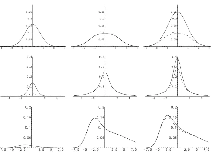
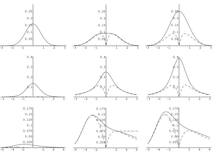
y _∈R(whenB ₆= 0). In this case the first order bias term cancels completely by the use of the empirical likelihood method. Also for examples of other distributions the new bias term can be considerably smaller. Figure 1 below shows curves for the squared bias, the variance and the mean squared error for normal distribution, student’s t-distribution with three degrees of freedom and the double exponential distribution with density

f(x) = 1 γ exp −x−_γ q×exp₋exp₋ x−q γ

for γ = 3 and q = ₋γc such that the expectation γc+q vanishes, where c= 0.5772 approx-imately, as skew distribution example (with E[ε3

1] 6= 0). We observe a bias reduction for all

three example distributions. INCLUDE FIGURE 1 HERE.

Example 5.2 In the case g(ε) = ε2 _−σ2 _{for known variance σ}2 _{we have E[g}0_(ε

1)] = 0 and

therefore both estimators have the same bias b(y) = b(y). The new variance is Var(G(y)) = F(y)(1₋F(y)) +f2(y)σ2+ 2f(y)E[ε1I{ε1 ≤y}]

−U2(y)Σ−1₋2f(y)U(y)Σ−1E[ε31].

For all distributions with vanishing third moment the new variance is uniformly smaller than Var(G(y)) and we obtain an improved estimator. In particular, for normally distributed errors we have

Var(G(y)) = Var(G(y))₋ 1 2y

Figure 2 below shows squared bias, variance and mean squared error curves for normal dis-tribution, student’s t-distribution with five degrees of freedom and the double exponential distribution defined in Example 5.1.

INCLUDE FIGURE 2 HERE.

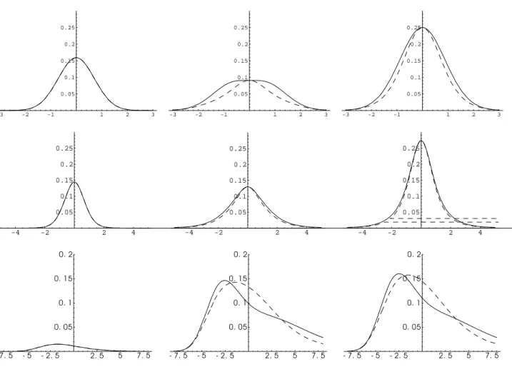
Example 5.3 The results obtained in Example 5.2 for a known variance can further be im-proved by including the information that the errors are centered and defining g(ε) = (ε, ε2₋ σ2₎T_{. Denoting µ} 3 = E[ε31], µ4 = E[(ε21 − σ2)2] and U1(y) = E[ε1I{ε1 ≤ y}], U2(y) = E[(ε2 1 −σ2)I{ε1≤y}] we obtain Var(G(y)) = F(y)(1₋F(y)) +f2(y)σ2+ 2f(y)E[ε1I{ε1 ≤y}] + 1 (σ2_µ 4−µ23)2 U₁2(y)µ4µ23+U22(y)(2σ2µ3−σ4µ4) −2U1(y)U2(y)µ33 + 2 σ2_µ 4−µ23 f(y)U1(y)µ23−U2(y)µ3σ2 = Var(G(y))₋U2 2(y) 1 µ4

where the last line only holds for distributions with vanishing third moment. In this case the variance reduces to the variance in Example 5.2. For the bias term we have

b(y) = h2Bf(y) + 1 σ2_µ 4−µ23 (U1(y)µ4−U2(y)µ3) .

For distributions with µ3 = 0 the bias is the same as in Example 5.1; in particular, it is

zero for normal distributions. For all distributions with vanishing third moment we therefore obtain an estimator with both smaller bias and smaller asymptotic variance. Figure 3 shows the corresponding squared bias, variance and mse curves for normal distribution, student’s

t-distribution with five degrees of freedom and double exponential distribution. For all three distributions we observe a considerably smaller mean squared error compared to Example 5.2. INCLUDE FIGURE 3 HERE.

Next, we consider an example corresponding to additional information about quantiles accord-ing to Theorem 3.7.

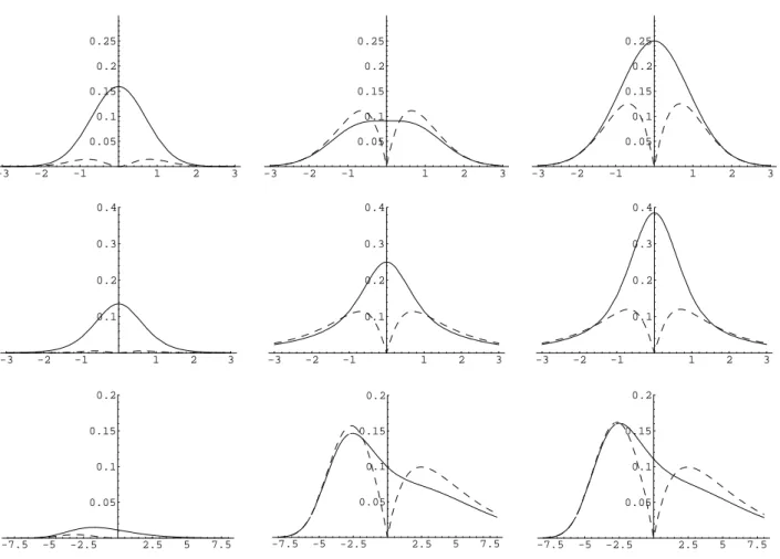
Example 5.4 For g(ε) = I_{ε _≤ a_{} −}b we obtain for distributions with zero median (a = 0, b = 0.5) the variance

+4h4U2(y)_{1 4 + 2f(0)E[ε1I{ε1 ≤0}] +f 2_(0)σ2 } −2U(y)(F(0_∧y)₋ 1 2F(y) +f(0)E[ε1I{ε1 ≤y}]) −2f(y)U(y)_{E[ε1I{ε1 ≤0}] +f(0)σ2} i with U(y) = F(0_∧y)₋ 1

2F(y)∈[0,0.25] for ally∈R. The bias is

b(y) = h2B(f(y)₋4U(y)f(0)) =h2B(f(y)₋4[F(0_∧y)₋ 1

2F(y)]f(0)).

Figure 4 below shows curves for the squared bias, the variance and the mean squared error for normal distribution, student’s t-distribution with three degrees of freedom (both with a = 0 and b= 0.5) and double exponential distribution (with a = 0 and b= 0.570371).

INCLUDE FIGURE 4 HERE.

Example 5.5 We investigate in this example whether including the centeredness information gives better results compared to Example 5.4, that is, we considerg(ε) = (ε, I_{ε_≤0_}−F(0))T_,

where F(0) is known. This situation is not covered by Theorems 3.3 and 3.7, but results can be derived in a complete analogous way. We obtain for the asymptotic variance,

Var(G(y)) = Var(G(y)) +V2(y)Var(G(0))₋2V(y)Cov(G(y), G(0)) where Var(G(y)) is defined in (1.3),

V(y) = σ 2_U 2(y)−U1(0)U1(y) σ2_{F(0)(1−F(0))−U}2 1(0) and U1(y) =E[ε1I{ε1 ≤y}],U2(y) = E[(I{ε1 ≤0} −F(0))I{ε1 ≤y}] = F(y∧0)−F(0)F(y).

For the bias we have

b(y) = h2_{Bf(y) +} U1(y){F(0)(1−F(0)) +U1(0)f(0)} −U2(y){U1(0) +σ2f(0)}

σ2_{F(0)(1−F(0))−U}2 1(0)

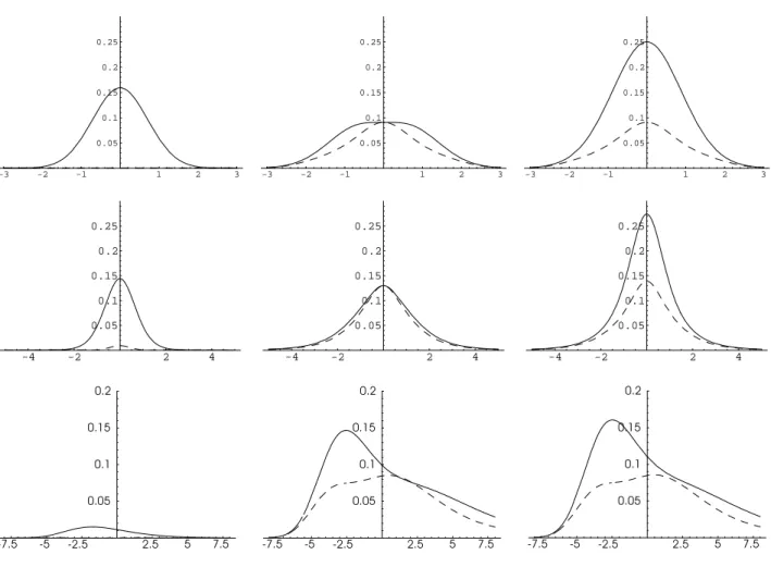
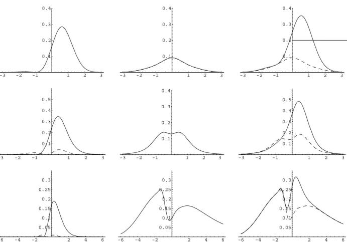
For standard normally distributed errors we have againb(y) = 0. Figure 5 below shows curves for the squared bias, the variance and the mean squared error for normal distribution, student’s

t-distribution with three degrees of freedom and the double exponential distribution. We obtain uniformly smaller mse’s for Fn compared with Example 5.4.

INCLUDE FIGURE 5 HERE.

Example 5.6 We consider the information function g(ε) = (ε, ε2₋₁₎T _{to include the model}

assumption of centered errors with unit variance into the error distribution estimation. This is comparable to Example 5.1 in the homoscedastic setting and analogously the asymptotic variance curves of ˆFn and Fn coincide whereas the new estimator has a smaller bias. In Figure

6 the squared bias, variance and mse curves are displayed for normal, student’s t-distribution with five degrees of freedom and double exponential distribution (all distributions standardized such that they are centered with unit variance).

INCLUDE FIGURE 6 HERE.

6

Small sample performance

In this section we compare the performances of the two distribution estimators for finite sam-ples by means of a simulation study. We concentrate on the homoscedastic model (2.1) with regression function m(x) = 3x2 _{and uniformly in [0,1] distributed design points. As error}

distributions we use the three different distributions already considered in section 5, namely standard normal distribution, student’s t-distribution and the double exponential distribution. For the regression estimator we use the standard normal kernel and we consider bandwidths

h = c/n1/4 _{according to the theoretical bandwidth conditions, for different suitable values of}

the constant c between 0.1 and 3. Displayed in Figures 7 and 8 are values of the mean inte-grated squared error E[R

(Gn(y)−F(y))2dy] for Gn = ˆFn and Gn =Fn, estimated from 1000

replications, where the integral is approximated using 100 grid points in an appropriate inter-val chosen as [₋3,3] for the normal distribution, [₋4,4] for the t-distribution and [₋7,7] for the double exponential distribution. For calculating ˆηn defined in (3.2) we used the Bisection

method for one-dimensional g and the multivariate Newton Raphson procedure otherwise [both described in Press, Teukolsky, Vetterling and Flannery (2002), p. 357 and p. 383].

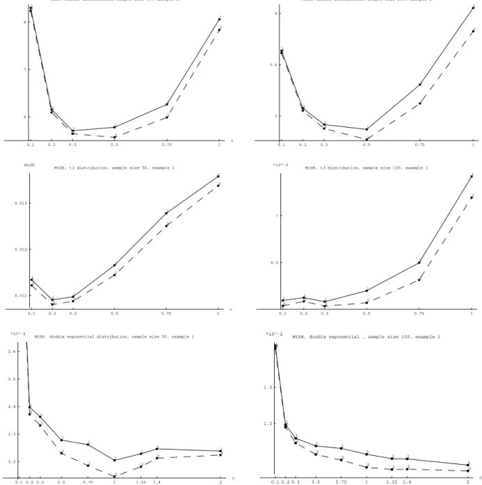
For Example 5.1, i. e. including the centeredness information, results are displayed in Figure 7. The sample size is n = 50 in the left column and n = 100 in the right column. In the first row the error distribution is standard normal. The solid curve (curve 1) displays the mean integrated squared error, or MISE, for the residual based empirical distribution function ˆFn,

whereas the dashed curve (curve 2) displays the corresponding results for the new estimator

Fn. We always obtain better results, i. e. a smaller MISE, for the new estimator, although

for some choices of bandwidths the values are very close. For the symmetric distributions it is interesting to see the effect that for an increasing bandwidth the difference between the performances of the two estimators increases. This is according to the theory because for an

increasing bandwidth the effect of the bias on the MISE increases and in this example the new estimator has a considerably smaller asymptotic bias. The results displayed in the second and third row of Figure 7 correspond to the student’s t-distribution with three degrees of freedom and the double exponential distribution, respectively. We obtain a smaller MISE for the new estimator in all cases.

INCLUDE FIGURE 7 HERE.

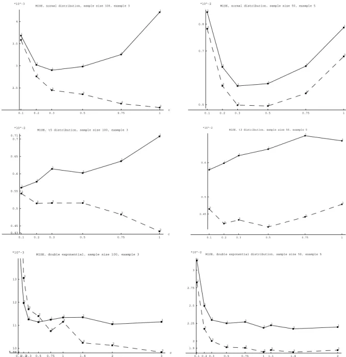
In Figure 8 the MISE curves for Example 5.3 are displayed in the left panel, where the sample size is n = 100 and we consider standard normal, t5 and double exponential distribution. For

standard normally and t–distributed errors the empirical likelihood methods yields a great improvement in terms of MISE. For double exponential distribution the new estimator has a smaller MISE only for bandwidth constants greater thanc= 0.5 and for this distribution larger bandwidths should be recommended. In the right panel of Figure 8 results for Example 5.5 for sample size n= 50 and normal, t3 and double exponential distribution are shown. In all cases

the new estimator has a smaller MISE.

INCLUDE FIGURE 8 HERE.

We also implemented an approximation of ˆηn from the asymptotic expansion given in

Proposi-tion 3.2, where only the dominating term is used. In most cases this gave even better results, but it failed to work in Example 5.3. Therefore, the results are not displayed and we do rec-ommend to use the Bisection or Newton Raphson procedure to obtain ˆηn instead of using the

approximation.

Acknowledgements. The authors would like to thank Ingrid Van Keilegom and Holger Dette for helpful discussions. The financial support by the Deutsche Forschungsgemeinschaft (SFB 475) is gratefully acknowledged. Part of this paper was written while the third author visited the Australian National University in Canberra and this author would like to thank the members of the Mathematical Science Institute, in particular Peter Hall, for their hospitality.

A

Appendix: Akritas and Van Keilegom’s process

The homoscedastic model

We give a short derivation of the results stated in the introduction, in particular (1.4) and (1.3). From the proof of Theorem 1 by Akritas and Van Keilegom (2001, p. 555) it follows that in the case of homoscedasticity (where no estimation of a variance function σ is needed) and for score function J =I[0,1] the functionϕ defined in Theorem 1 (p. 552) has the form

ϕ(x, z, y) = ₋f(y) Z

(I_{z _≤v_{} −}F(v_|x))dv.

Here, F(v_|x) =F(v₋m(x)) is the conditional distribution of Yi given Xi =x and we obtain

ϕ(x, z, y) = ₋f(y) Z ∞ z (1₋F(v_|x))dv₋ Z z −∞ F(v_|x)dv = ₋f(y)(m(x)₋z).

Therefore, ϕ(Xi, Yi, y) =f(y)εi and (1.3) follows from Theorem 2 by Akritas and Van Keilegom

(2001, p. 552). The bias formula (1.4) is deduced from the bias of the Nadaraya–Watson [Nadaraya (1964), Watson (1964)] regression estimator and the expansion

ˆ

Fn(y)−F(y) = Fn(y)−F(y) +f(y)

Z

( ˆm(x)₋m(x))fX(x)dx+oP(n−1/2)

where Fn denotes the empirical distribution function of the true errors [see p. 555 of Akritas

and Van Keilegom (2001)].

The heteroscedastic model

In the heteroscedastic model (4.1) the functionϕfrom Theorem 1 by Akritas and Van Keilegom (2001) is equal to ϕ(x, z, y) = ₋ f(y) σ2_(x) σ(x)(m(x)₋z)₋ym2(x) +ym(x)z+ 1 2σ 2_(x)y+1 2m 2_(x)y − 1₂yz2

and this yields ϕ(Xi, Yi, y) =f(y)(εi+y₂(ε2i −1)). The bias b(y) is deduced from the expansion

ˆ Fn(y)−F(y) = Fn(y)−F(y) +f(y) Z _mˆ(x) −m(x) σ(x) fX(x)dx +yf(y) Z ˆ σ(x)₋σ(x) σ(x) fX(x)dx+oP(n −1/2₎ = Fn(y)−F(y) +f(y) Z ˆ m(x)₋m(x) σ(x) fX(x)dx +yf(y) Z ˆ σ2_(x)−σ2_(x) 2σ2_(x) fX(x)dx+oP(n −1/2₎

[compare p. 555, 564, Akritas and Van Keilegom (2001)] by inserting the definitions of ˆm in (2.2) and ˆσ2 _{in (4.3).}

B

Appendix: Auxiliary results

Lemma B.1 Assume model (2.1) with assumptions (M1), (M2), (K), (H) and (A).

(i) With either g(ε) = I_{ε_≤a_{} −}b for some constants a and b (k= 1) org satisfying (G1) and (G2) we have maxi=1,...,n|gj(ˆεi)|=oP(√n) (j = 1, . . . , k).

(ii) Under the additional assumptions (G1), (G2) we have the expansion 1

n Pn i=1gj(ˆεi) = 1 n Pn i=1(gj(εi)−E[gj0(ε1)]εi)−h2E[gj0(ε1)]B+oP(√1_n) (j = 1, . . . , k) where B is defined in Theorem 3.3.

(iii) For g(ε) = I_{ε _≤ a_{} −} b for some constants a and b (k = 1) we have the expansion

1 n Pn i=1g(ˆεi) = 1 n Pn i=1g(εi) +f(a)εi+h2f(a)B+oP( 1 √

n) where B is defined in Theorem

3.3.

(iv) With either g(ε) = I_{ε_≤a_{} −}b for some constants a and b (k= 1) org satisfying (G1) and (G2) we have _n1Pn

i=1(gj(ˆεi)−gj(εi))2 =oP(1)(j = 1, . . . , k).

(v) With either g(ε) = I_{ε_≤a_{} −}b for some constants a and b (k= 1) org satisfying (G1) and (G2) we have 1

n

Pn

i=1g(ˆεi)gT(ˆεi) = Σ +oP(1).

Proof. (i). Under the assumptions, condition (2.4) is valid. We have from the triangle inequality

max

i=1,...,n|gj(ˆεi)| ≤ i=1max,...,n|gj(ˆεi)−gj(εi)|+ maxi=1,...,n|gj(εi)|

(B.1)

and consider the second term on the right hand side first. For every >0 one obtains

P max i=1,...,n|gj(εi)|> √ n _≤ nE[I_{|gj(ε1)|> √n}] (B.2) ≤ 1 2E h |gj(ε1)|2I{|gj(ε1)|2 ≥2n} i = o(1) with the assumption E[g2

j(ε1)] < ∞. For the first term on the right hand side of (B.1) we

further have P max i=1,...,n|gj(ˆεi)−gj(εi)|> √ n _≤ P max i=1,...,n|gj(ˆεi)−gj(εi)|> √ n, max i=1,...,n|εi−εˆi| ≤δ +P max i=1,...,n|εi−εˆi|> δ

[with δ from condition (2.4)]. The last probability converges to zero because max

i=1,...,n|εi−εˆi| ≤_xsup_∈[0,1]|mˆ(x)−m(x)|=o(1)

(B.3)

almost surely by assumptions (M1), (M2), (K) and (H). Furthermore we have

P max i=1,...,n|gj(ˆεi)−gj(εi)|> √ n, max i=1,...,n|εi−εˆi| ≤δ ≤ P max i=1,...,n|hj(εi)|> √ n

where hj(x) = supy∈R:|y|≤δ|gj(x+y)−gj(x)|. Analogous to argumentation (B.2) we obtain the

assertion from (2.4), that is E[h2

j(ε1)]<∞.

(ii). This statement corresponds to Theorem 2 by M¨uller, Schick and Wefelmeyer (2004a) when using a leave-one-out local polynomial estimator for the regression function. We present a different proof nevertheless because some arguments of the proof are used to show (iv) and (v). Our proof uses some ideas of the proof of Lemma 1, Akritas and Van Keilegom (2001). First, we show weak convergence of the empirical process

Gn(˜gj) = 1 √ n n X i=1 ˜ gj(εi, Xi)− Z Z ˜ gj(y, x)f(y)fX(x)dy dx (B.4)

indexed by functions ˜gj ∈ Gj, where

Gj = n ˜ gj :R×[0,1]→R,g˜j(ε, x) = gj(ε+h(x))−gj(ε) h∈ H o . (B.5)

The smooth function class _H = C_δ1+α[0,1] is defined in van der Vaart and Wellner (1996, p. 154) [see also the proof of Lemma D.1: all continuous functions h: [0,1]_→IRthat fulfill (D.1) build the class C1+α

ρ [0,1]]. Note that forn → ∞the functionm−mˆ is an element ofCδ1+α[0,1]

with probability one [confer Akritas and Van Keilegom (2001)] and that 1 n n X i=1 gj(ˆεi) = 1 n n X i=1 gj(εi+ (m−mˆ)(Xi)).

The function class _Gj has a square integrable envelope by (2.4) because supx∈[0,1]|h(x)| ≤δ for

h _{∈ H}. In order to show that_Gj is Donsker we prove that the bracketing integral is finite, i. e.

Z ∞

0

q

logN[ ](ξ,Gj, L2(P))dξ <∞,

(B.6)

whereP denotes the distribution of (ε1, X1). Letξ >0 and define ˜ξ= (ξ/(2C))κ with constant

C defined in assumption (G2). We have from Theorem 2.7.1 in van der Vaart and Wellner (1996, p. 155) for the covering numbers of _H with respect to the supremum norm,

logN( ˜ξ,_H,_{|| · ||∞})_≤Kξ−κ/(1+α)

for some constant K. Further, for ˜ξ _≥δthe covering number is one, choosing the centerh1 ≡0

and noting that supx∈[0,1]|h(x)| ≤δ for h∈ H. Let h1, . . . , hλ [λ=N( ˜ξ,H,|| · ||∞)] denote the

centers of a covering for _H with radius ˜ξ with respect to the supremum norm. Let h _{∈ H} and ||h₋hi||∞<ξ˜. Then a bracket for ˜gj(ε, h) = gj(ε+h(x))−gj(ε) is given by

h

gj(ε+hi(x))−gj(ε)−g˜∗j(ε, x), gj(ε+hi(x))−gj(ε) + ˜gj∗(ε, x)

i

where ˜g_j∗(ε, x) = sup_|gj(ε +z) −gj(ε + ˜z)| and the supremum is built over |z| ≤ δ,|z˜| ≤

δ,_|z₋z˜_{| ≤} ξ˜. The bracket has L2(P) length less or equal to ξ by assumption (G2). We have

N[ ](ξ,Gj, L2(P)) =λ brackets and (B.6) follows from (B.7) and the assumption ₂₍₁₊κ_α) <1 [the

integral only has to be evaluated in (0,2Cδ1/κ_)].

We have shown weak convergence of the process Gn(˜gj) defined in (B.4) and insert the random

function ˆgj(ε, x) = gj(ε+ (m−mˆ)(x))−gj(ε) now. We have

Z ˆ g2_jdP = Z Z gj(y+ (m−mˆ)(x))−gj(y) 2 fX(x)f(y)dx dy = oP(1) (B.8)

by the dominated convergence theorem using (2.4) and the convergence R

(gj(y+ (m−mˆ)(x))−gj(y))2fX(x)dx −→ 0 for each fixed y (follows by Taylor’s

expan-sion and the almost sure uniform convergence of ˆm₋m to zero, because g0

j is continuous and

therefore bounded in a neighbourhood of the fixed y). By (B.8), applying Lemma 19.24 of van der Vaart (1998, p. 280) we obtain

Gn(ˆgj) = 1 √_n n X i=1 gj(εi+ (m−mˆ)(Xi))−gj(εi) − Z Z (gj(y+ (m−mˆ)(x))−gj(y))fX(x)f(y)dx dy =oP(1).

By assumptions (G1) and (H) using sup_x∈[0,1]|mˆ(x)₋m(x)_| =O((n−1_h−1_logh−1₎1/2_{) a.s. [confer}

Prop. 3, Akritas and Van Keilegom (2001)] we obtain the expansion 1 √ n n X i=1 gj(εi+ (m−mˆ)(Xi)) = 1 √ n n X i=1 gj(εi) +√n Z (m₋mˆ)(x)fX(x)dx Z g0j(y)f(y)dy+oP(1).

The assertion now follows by inserting the definition of ˆm in (2.2) and tedious but simple calculations of expectations and variances using assumptions (K) and (H).

(iii). This follows like Theorem 1 of Akritas and Van Keilegom (2001) in a homoscedastic model, compare appendix A.

(iv). The proof uses results from the proofs of (ii) and (iii). The function class _Gj defined in

(B.5) is Donsker (in either case for g) and therefore_G2

j is Glivenko–Cantelli class in probability

[van der Vaart and Wellner (1996, p. 194, Lemma 2.10.14) ]. We obtain sup h∈H 1 n n X i=1 gj(εi+h(Xi))−gj(εi) 2 − Z Z gj(y+h(x))−gj(y) 2 fX(x)f(y)dx dy = op(1) and therefore 1 n n X i=1 gj(εi+ (m−mˆ)(Xi))−gj(εi) 2 = Z Z gj(y+ (m−mˆ)(x))−gj(y) 2 fX(x)f(y)dx dy+oP(1).

The assertion follows from (B.8) in the case of a smooth function gand the analogous statement for the indicator function g(ε) =I_{ε_≤a_{} −}b. The latter is obtained by

Z Z

(g(y+ (m₋mˆ)(x))₋g(y))2fX(x)f(y)dx dy =

Z

|F(a+ ( ˆm₋m)(x))₋F(a)_|fX(x)dx,

assumption (M3) and sup_x∈[0,1]|mˆ(x)₋m(x)_|=o(1) almost surely. (v). For j, `_{∈ {}1, . . . , k_} we have to show that

1 n n X i=1 gj(ˆεi)g`(ˆεi) = Z gj(y)g`(y)f(y)dy+oP(1).

The proof is similar to the proof of (iv). The function classes ˜

Gj = {(ε, x)7→gj(ε+h(x))|h∈ H}

are Donsker (j = 1, . . . , k) (where _H=C_δ1+α[0,1]). From van der Vaart and Wellner (1996, p. 204, Problem 8) follows that ˜_GjG˜` is Glivenko–Cantelli class in probability. From this follows

sup h∈H 1 n n X i=1 gj(εi+h(Xi))g`(εi+h(Xi))−E[gj(ε1+h(X1))g`(ε1+h(X1))] = oP(1)

and therefore we have with ˆεi =εi+ (m−mˆ)(Xi)

1 n n X i=1 gj(ˆεi)g`(ˆεi)− Z Z gj(y+ (m−mˆ)(x))g`(y+ (m−mˆ)(x))fX(x)f(y)dx dy = oP(1).

From sup_x∈[0,1]|mˆ(x)₋m(x)_|=o(1) almost surely we obtain the assertion similar to (B.8) and the considerations at the end of the proof of (iv). 2

Lemma B.2 Under assumptions (M1), (M2), (K), (H), (A), (S1) and (S2) we have (i) _||ηˆn||=OP(1/√n) (ii) max i=1,...,n 1 1 + ˆηT ng(ˆεi) =OP(1).

Proof. (i). ηˆn is the solution of equation (3.2). From this we obtain the estimation

0 = 1 n n X i=1 g(ˆεi) 1 + ˆηT ng(ˆεi) = 1 n n X i=1 g(ˆεi)− 1 n n X i=1 ˆ ηnTg(ˆεi) g(ˆεi) 1 + ˆηT ng(ˆεi) ≥ ||ηˆn|| 1 n n X i=1 ||g(ˆεi)||2 1 1 +_||ηˆn|| max j=1,...,ki=1max,...,n|gj(ˆεi)| − 1 n n X i=1 g(ˆεi)

and it follows that ||ηˆn|| ≤ 1 n n X i=1 g(ˆεi) 1 n n X i=1 ||g(ˆεi)||2− 1 n n X i=1 g(ˆεi) _jmax_=1,...,ki=1max_,...,n|gj(ˆεi)| −1 .

Now from Lemma B.1 (iv) we have that 1

n Pn i=1||g(ˆεi)||2 = n1 Pn i=1g21(ˆεi)+. . .+gk2(ˆεi) converges in probability to E[g2

1(ε1) +. . .+gk2(ε1)]>0 by assumption (S2). From Lemma B.1 (i) and (ii)

resp. (iii) follows the assertion.

(ii). In order to prove the assertion we show max1≤i≤n|1−(1+ ˆηnTg(ˆεi))−1|=oP(1). By Lemma

B.1(i) and Lemma B.2(i) we have P(_||ηˆn||max1≤i≤n,1≤j≤k|gj(ˆεi)| ≥1) = o(1) and, further, for

all >0, Pmax 1≤i≤n ˆ ηT ng(ˆεi) 1 + ˆηT ng(ˆεi) > , ||ηˆn||₁ max ≤i≤n,1≤j≤k|gj(ˆεi)|<1 ≤ P ||ηˆn||max1≤i≤n,1≤j≤k|g(ˆεi)| 1_{− ||}ηˆn||max1≤i≤n,1≤j≤k|g(ˆεi)| > = P_||ηˆn|| max 1≤i≤n,1≤j≤k|g(ˆεi)|> 1 + = o(1). 2 Lemma B.3 Under model (2.1) and assumptions (M1), (M2), (M3), (K), (H) and (A) we have sup y∈R 1 n n X i=1 |I_{εˆi ≤y} −I{εi ≤y}|=oP(1).

Proof. The assertion is shown in two steps. The first step consists in showing 1

n

Pn

i=1|I{εˆi ≤

I_{y₋τ < εi ≤ y+τ} for τ > 0 for all i = 1, . . . , n, y ∈ R whenever max1≤i≤n|εˆi −εi| ≤ τ.

Hence, for any >0 we have

P1 n n X i=1 |I_{εˆi ≤y} −I{εi ≤y}|> ≤ P 1 n n X i=1 I_{y₋τ < εi≤y+τ} −(F(y+τ)−F(y−τ)) > /2 (B.9) +P(_|F(y+τ)₋F(y₋τ)_|> /2) +P( max 1≤i≤n|εˆi−εi| > τ). (B.10)

The term (B.9) converges to zero almost surely according to the strong law of large numbers. Because F is continuous the first term in term (B.10) is equal to zero for some sufficiently small

τ. The second term in (B.10) converges to zero because of (B.3).

After showing the assertion for fixed y we include the supremum by a standard argument. The distribution function F is continued with F(_−∞) := 0, F(_∞) := 1. Then the real line is segmented into _−∞=y0 < y1 < . . . < yN−1 < yN =∞ such that|F(yk)−F(yk−1)| < /2 for

k = 1, . . . , N. For eachyexists ak _{∈ {}1, . . . , N_}such that y_∈[yk−1, yk). The assertion follows

using _|I_{εi ≤ y} −I{εˆi ≤y}| ≤ |I{εˆi ≤yk} −I{εi ≤yk−1}|+|I{εˆi ≤yk−1} −I{εi ≤yk}| for

an estimation of 1_nPn

i=1|I{εi ≤y} −I{εˆi ≤y}| through expressions with fixed yk,1≤k ≤N,

using the first part of the proof. 2

C

Appendix: Proofs of main results

Proof of Proposition 3.1

ηn is a solution of equation (3.2) and this yields

0 = 1 n n X i=1 g(ˆεi)− 1 n n X i=1 g(ˆεi)g(ˆεi)Tηˆn+ 1 n n X i=1 (ˆη_nTg(ˆεi))2 g(ˆεi) 1 + ˆηT ng(ˆεi) . (C.1)

The last term can be estimated as follows, 1 n n X i=1 (ˆη_nTg(ˆεi))2 g(ˆεi) 1 + ˆηT ng(ˆεi) ≤ ||ηˆn||2 1 n n X i=1 ||g(ˆεi)||2 max j=1,...,ki=1max,...,n|gj(ˆεi)|i=1max,...,n 1 1 + ˆηT ng(ˆεi) =oP( 1 √ n)

using Lemma B.2 (i), (ii), Lemma B.1 (i) and (v). In the second term of (C.1) we can replace

1

n

Pn

Proof of Proposition 3.2

We use the following expansion similar to the beginning of the proof of Prop. 3.1,

Fn(y)−Fˆn(y) = − 1 n n X i=1 ˆ ηT ng(ˆεi) 1₋ηˆT ng(ˆεi) + (ˆηT ng(ˆεi))2 1 + ˆηT ng(ˆεi) I_{εˆi ≤y}.

To prove the assertion of the Proposition we have to show uniformly with respect to y_∈R

1 n n X i=1 g(ˆεi)I{εˆi ≤y} = U(y) +oP(1) (C.2) 1 n n X i=1 (ˆη_nTg(ˆεi))2I{εˆi ≤y} = oP( 1 √ n) (C.3) 1 n n X i=1 (ˆηT ng(ˆεi))3 1 + ˆηT ng(ˆεi) I_{εˆi ≤y} = oP( 1 √ n). (C.4)

To show (C.2) we use the expansion 1_nPn

i=1g(ˆεi)I{εˆi ≤y}=An(y) +Bn(y) +Cn(y), where An(y) = 1 n n X i=1 g(εi)I{εi ≤y} Bn(y) = 1 n n X i=1 (g(ˆεi)−g(εi))I{εˆi ≤y} Cn(y) = 1 n n X i=1 g(εi)(I{εˆi ≤y} −I{εi ≤y}).

An(y) converges uniformly toU(y) almost surely, because the class{ε7→g(ε)I{ε≤y} |y∈R}

is VC-subgraph [see van der Vaart and Wellner (1996), Lemma 2.6.18 (vi), p. 147] and therefore forms a Glivenko–Cantelli class. Further we have uniformly in y_∈R

||Bn(y)|| ≤ 1 n n X i=1 ||g(ˆεi)−g(εi)||2 1/21 n n X i=1 I_{εˆi ≤y} 1/2 ≤ 1 n n X i=1 (g1(ˆεi)−g1(εi))2+. . .+ (gk(ˆεi)−gk(εi))2 1/2 =oP(1) by Lemma B.1 (v). Furthermore, ||Cn(y)|| ≤ 1 n n X i=1 ||g(εi)||2 1/21 n n X i=1 (I_{εˆi ≤y} −I{εi ≤y})2 1/2 = OP(1) 1 n n X i=1 |I_{εˆi ≤y} −I{εi ≤y}| 1/2 = oP(1)

by Lemma B.3. The next assertion, (C.3), is valid because 1 n n X i=1 (ˆη_nTg(ˆεi))2I{εˆi ≤y} ≤ ||ηˆn||2 1 n n X i=1 ||g(ˆεi)gT(ˆεi)||=OP(n−1)OP(1) =oP(n−1/2)

according to Lemma B.1(iv) and Lemma B.2. The assertion (C.4) is valid because it holds that |_n1 n X i=1 (ˆηT ng(ˆεi))3 1 + ˆηT ng(ˆεi) I_{εˆi ≤y}| ≤ ||ηˆn||3 max 1≤i≤n,1≤j≤k|gj(ˆεi)|1max≤i≤n 1 1 + ˆηT ng(ˆεi) 1 n n X i=1 ||g(ˆεi)gT(ˆεi)||=oP(n−1)

using Lemma B.2 (i) and (ii), Lemma B.1 (i) and (v). 2

Proof of Theorem 3.3

The expansion of the process follows from Propositions 3.2, 3.1 and Lemma B.1 (ii). Because sums of Donsker classes are Donsker [van der Vaart and Wellner (1996), p. 192, Ex. 2.10.7.] we only need to show that the following function classes _F` (`= 1,2) are Donsker,

F1 = {ε7→I{ε ≤y} −F(y)|y∈R}

F2 = {ε7→f(y)ε−U(y)TΣ−1(g(ε)−E[g0(ε1)]ε)|y∈R}.

F1 is Donsker by classical results. F2 is a subset of the at most (k+ 1)-dimensional vector space

{ε _7→ c0ε+Pk_j=1cjhj(ε) | c0, . . . , ck ∈ R} (with hj(ε) = gj(ε)−E[gj0(ε1)]ε) and is therefore

a VC-class [van der Vaart and Wellner (1996), p. 146, Lemma 2.6.15]. Pointwise separability of _F2 can be shown by a standard argument considering the countable subclass indexed by

rational y _∈ Q. Moreover, _F2 has a square integrable envelope by assumptions (M2) and (A)

and is therefore Donsker [van der Vaart and Wellner (1996), p. 141].

For the calculation of the covariances denoteHi(y) :=I{εi ≤y}−F(y)+f(y)εi−U(y)TΣ−1(g(εi)−

E[g0_(ε

1)]εi) so that √n(Fn(y)−F(y)−b(y)) = √1_nPn_i=1Hi(y) +op(1) and E[H1(y)] = 0. For

the covariance one obtains Cov(_√1 n n X i=1 Hi(y), 1 √_n n X j=1 Hj(z)) =E[H1(y)H1(z)] = E[(I_{ε1 ≤y} −F(y))(I{ε1≤z} −F(z))] +f(y)f(z)E[ε21] +U(y)TΣ−1E[(g(ε1)−E[g0(ε1)]ε1)(g(ε1)−E[g0(ε1)]ε1)T]U(z)Σ−1

+E[(I_{ε1 ≤y} −F(y))f(z)ε1] +E[(I{ε1 ≤z} −F(z))f(y)ε1]

−E[(I_{ε1 ≤y} −F(y))U(z)TΣ−1(g(ε1)−E[g0(ε1)]ε1)]

−E[(I_{ε1 ≤z} −F(z))U(y)TΣ−1(g(ε1)−E[g0(ε1)]ε1)]

−E[f(y)ε1U(z)TΣ−1(g(ε1)−E[g0(ε1)]ε1)]

−E[f(z)ε1U(y)TΣ−1(g(ε1)−E[g0(ε1)]ε1)]

which coincides with the asserted asymptotic covariance in Theorem 3.3. 2

Proof of Theorem 3.7

Using Propositions 3.2, 3.1 and Lemma B.1 (iii) the proof follows analogously to the proof of

Theorem 3.3. 2

D

Appendix: Proofs for the heteroscedastic model

Let K1, K2 > 0 denote constants such that 2K1 ≤ σ(x) ≤ K2/2 for all x ∈ [0,1] and the

derivatives σ0 _{and σ}00 _{are also bounded by K}

2/2 according to assumption (M). Then it follows

that P(K1 ≤σˆ(x)≤K2 for all x∈[0,1]) converges to one. From the argumentation in Akritas

and Van Keilegom (2001) we have that ˆm₋m and ˆσ₋σ are elements ofC1+α

ρ [0,1] for allρ >0

forn _{→ ∞}with probability one. A suitable choice ofρyields that ( ˆm₋m)/σˆand (ˆσ₋σ)/σˆ are elements of_H =C_δ1+α[0,1] with constantδfrom assumption (G2’), forn _{→ ∞}with probability one. This is assured by the next Lemma and is needed in the proof of Proposition 4.1.

Lemma D.1 Let δ > 0 and K1, K2 > 0 such that s ∈ CK1+2α[0,1] with infx∈[0,1]|s(x)| ≥ K1.

Then there exists some ρ >0 such that h_{s ∈}C_δ1+α[0,1]for all h_∈C1+α ρ [0,1].

Proof. Leth_∈C1+α

ρ [0,1]. Then from the definition of the function class we have that

max sup x∈[0,1]| h(x)_|, sup x∈[0,1]| h0(x)_|+ sup x,y∈[0,1] |h0_(x)−h0_(y)| |x₋y_|α ≤ ρ (D.1)

[van der Vaart and Wellner (1996, p. 154)] and the analogous inequality for function s and constant K2. From this and the boundedness of s by K1 from above it follows with technical

but straightforward estimations omitted for the sake of brevity that max sup x∈[0,1] h s(x) , sup x∈[0,1] ( h s) 0_(x) + sup x,y∈[0,1] |(h s)0(x)−( h s)0(y)| |x₋y_|α ≤ cρ

with some constant c only dependent on K1, K2. The assertion follows by the choice ρ = δ/c

Proof of Proposition 4.1

The proof follows the lines of the proof of Lemma B.1 (ii). The function classes _Gj [compare

(B.5)] is now defined as Gj = n ˜ gj :R×[0,1]→R,˜gj(ε, x) = gj(ε+h1(x) +εh2(x))−gj(ε) h1, h2 ∈ H o ,

where _H = C_δ1+α[0,1] with constant δ from assumption (G2’). We show in the following that _Gj is Donsker. To this end let for ξ > 0, as in the proof of Lemma B.1 (ii), h1, . . . , hλ

[λ = N( ˜ξ,_H,_{|| · ||∞})] denote the centers of a supremum-norm covering for _H with radius ˜

ξ = (ξ/(2C))κ _{with constant C from assumption (G2’). Then we have N}

[ ](ξ,Gj, L2(P)) = λ2 brackets h gj(ε+h`(x) +εhk(x))−gj(ε)−˜gj∗(ε, x), gj(ε+h`(x) +εhk(x))−gj(ε) + ˜gj∗(ε, x) i , `, k _{∈ {}1, . . . , λ_}, where ˜g_j∗(ε, x) = sup_|gj(ε+z1+εz2)−gj(ε+ ˜z1+εz˜2)| and the supremum is

built over _|z1|,|z2|,|z˜1|,|z˜2| ≤δ,|z1−z˜1|,|z2−z˜2| ≤ ξ˜. Each bracket has L2(P) length less or

equal to ξ by assumption (G2’). The bracketing integral (B.6) is finite with the same reasoning as in the proof of Lemma B.1 (ii).

Now, from Lemma D.1 we have that the probability that ( ˆm₋m)/σˆ _{∈ H} and (ˆσ₋σ)/σˆ _{∈ H} converges to one. The rest of the proof follows as the proof of Lemma B.1 (ii) leading to the expansion 1 n n X i=1 gj(ˆεi) = 1 n n X i=1 gj εi+ (m₋mˆ)(x) ˆ σ(x) +εi (σ₋σˆ)(x) ˆ σ(x) = 1 n n X i=1 gj(εi) +oP(n−1/2) + Z Z gj y+ (m−mˆ)(x) ˆ σ(x) +y (σ₋σˆ)(x) ˆ σ(x) −gj(y) fX(x)f(y)dx dy.

By assumption (G1’) we further obtain 1 n n X i=1 gj(ˆεi) = 1 n n X i=1 gj(εi) + Z Z g_j0(y)m(x)−mˆ(x) ˆ σ(x) fX(x)f(y)dx dy + Z Z g_j0(y)yσ(x)−ˆσ(x) ˆ σ(x) fX(x)f(y)dx dy+oP(n −1/2₎ = 1 n n X i=1 gj(εi)−E[gj0(ε1)] Z ˆ m(x)₋m(x) σ(x) fX(x)dx −E[ε1g0j(ε1)] Z ˆ σ2_(x)−σ2_(x) 2σ2_(x) fX(x)dx+oP(n− 1/2_),

where the last equality follows from the uniform almost sure convergence of ˆσ to σ with rate

O((n−1_h−1_logh−1₎1/2_{) [confer Prop. 3, Akritas and Van Keilegom (2001)], the bandwidth}

con-ditions (H), and ˆσ ₋σ = (ˆσ2 _−σ2_{)/(2σ)−(ˆσ −σ)}2_{/(2σ), where the last term results in a}

negligible remainder. The rest of the proof follows by inserting the definitions of ˆm from (2.2), ˆ

σ2 _{from (4.3), and some straightforward calculations of expectations and variances.}

2

Proof of Theorem 4.2

The validity of Propositions 3.1 and 3.2 in the heteroscedastic model (4.1) under the assump-tions of Theorem 4.2 can be shown following the steps of the proofs for the homoscedastic case. To this end one shows that Lemmas B.1 (i), (vi), (v), B.2 and B.3 hold as well under these assumptions. The proofs are analogous, using the following estimation for Lemmas B.1 (i) and B.3 and noting that (G2) follows from (G2’). We have

max i=1,...,n|εi−εˆi| ≤ _xsup_∈[0,1]| ˆ m(x)₋m(x) ˆ σ(x) |+ maxi=1,...,n|εi|_xsup_∈[0,1]| ˆ σ(x)₋σ(x) ˆ σ(x) | = oP(1)

where the last equality follows from maxi=1,...,n|εi|=oP(n1/4) under assumption (M), the

uni-form rates of convergence, sup_x∈[0,1]|mˆ(x)₋m(x)_| =O((n−1_h−1_logh−1₎1/2_{) and sup}

x∈[0,1]|σˆ(x)−

σ(x)_| = O((n−1_h−1_logh−1₎1/2_{) a.s. [confer Prop. 3, Akritas and Van Keilegom (2001)], the}

boundedness of σ from zero, and the bandwidth conditions (H).

The rest of the proof is exactly the same as the proof of Theorem 3.3. 2

E

References

M. Akritas and I. Van Keilegom (2001). Nonparametric estimation of the residual distri-bution. Scand. J. Statist. 28, 549–567.

H. Bonnal, E. Renault (2004). On the Efficient Use of the Informational Content of Esti-mating Equations: Implied Probabilities and Euclidean Empirical Likelihood. Technical report. http://ideas.repec.org/p/cir/cirwor/2004s-18.html

F. Cheng (2004). Weak and strong uniform consistency of a kernel error density estimator in nonparametric regression. J. Statist. Plann. Inference 119, 95–107.

F. Cheng (2002). Consistency of error density and distribution function estimators in non-parametric regression. Statist. Probab. Lett. 59, 257–270.