10-2018
Estimation of area under the ROC curve under
nonignorable verification bias
Wenbao Yu
Children's Hospital of Philadelphia
Jae Kwang Kim
Iowa State University, jkim@iastate.edu
Taesung Park
Seoul National University
Follow this and additional works at:
https://lib.dr.iastate.edu/stat_las_pubs
Part of the
Diseases Commons
,
Probability Commons
, and the
Statistical Methodology
Commons
The complete bibliographic information for this item can be found at
https://lib.dr.iastate.edu/
stat_las_pubs/260
. For information on how to cite this item, please visit
http://lib.dr.iastate.edu/
howtocite.html
.
This Article is brought to you for free and open access by the Statistics at Iowa State University Digital Repository. It has been accepted for inclusion in Statistics Publications by an authorized administrator of Iowa State University Digital Repository. For more information, please contact
Estimation of area under the ROC curve under nonignorable verification
bias
Abstract
The Area Under the Receiving Operating Characteristic Curve (AUC) is frequently used for assessing the overall accuracy of a diagnostic marker. However, estimation of AUC relies on knowledge of the true
outcomes of subjects: diseased or non-diseased. Because disease verification based on a gold standard is often expensive and/or invasive, only a limited number of patients are sent to verification at doctors discretion. Estimation of AUC is generally biased if only small verified samples are used and it is thus necessary to make corrections for such lack of information. Correction based on the ignorable missingness assumption (or missing at random) is also biased if the missing mechanism depends on the unknown disease outcome, which is called nonignorable missing. In this paper, we propose a propensity-score-adjustment method for
estimating the AUC based on the instrumental variable assumption when the missingness of disease status is nonignorable. The new method makes parametric assumptions on the verification probability, and the probability of being diseased for verified samples rather than for the whole sample. The proposed parametric assumption on the observed sample is easier to be verified than the parametric assumption on the full sample. We establish the asymptotic properties of the proposed estimators. A simulation study was performed to compare the proposed method with existing methods. The proposed method is applied to an Alzheimers disease data collected by National Alzheimers Coordinating Center.
Keywords
Instrumental variable, missing data, not missing at random, ROC curve Disciplines
Diseases | Probability | Statistical Methodology Comments
This article is published as Yu, Wenbao, Jae Kwang Kim, and Taesung Park. "Estimation of Area Under the ROC Curve under nonignorable verification bias."Statistica Sinica28, no. 4 (2018): 2149. doi:10.5705/ ss.202016.0315. Posted with permission.
doi:https://doi.org/10.5705/ss.202016.0315
ESTIMATION OF AREA UNDER THE ROC CURVE UNDER NONIGNORABLE VERIFICATION BIAS
Wenbao Yu, Jae Kwang Kim and Taesung Park
Children’s Hospital of Philadelphia, Iowa State University and Seoul National University
Abstract: The Area Under the Receiving Operating Characteristic Curve (AUC) is frequently used for assessing the overall accuracy of a diagnostic marker. However, estimation of AUC relies on knowledge of the true outcomes of subjects: diseased or non-diseased. Because disease verification based on a gold standard is often ex-pensive and/or invasive, only a limited number of patients are sent to verification at doctors’ discretion. Estimation of AUC is generally biased if only small verified samples are used and it is thus necessary to make corrections for such lack of in-formation. Correction based on the ignorable missingness assumption (or missing at random) is also biased if the missing mechanism depends on the unknown dis-ease outcome, which is called nonignorable missing. In this paper, we propose a propensity-score-adjustment method for estimating the AUC based on the instru-mental variable assumption when the missingness of disease status is nonignorable. The new method makes parametric assumptions on the verification probability, and the probability of being diseased for verified samples rather than for the whole sample. The proposed parametric assumption on the observed sample is easier to be verified than the parametric assumption on the full sample. We establish the asymptotic properties of the proposed estimators. A simulation study was per-formed to compare the proposed method with existing methods. The proposed method is applied to an Alzheimer’s disease data collected by National Alzheimer’s Coordinating Center.
Key words and phrases: Instrumental variable, missing data, not missing at ran-dom, ROC curve.
1. Introduction
The Receiving Operating Characteristic (ROC) curve is a tool for evaluating the accuracy of a diagnostic marker. The area under the curve (AUC) is a pop-ular summary index for evaluating a method’s power of discriminating diseased from non-diseased subjects; it is the probability that the score of a randomly chosen diseased individual exceeds that of a randomly chosen non-diseased sub-jects (Bamber (1975)). Estimation of the AUC relies on knowledge of the true
status of subjects, which can usually be verified through a gold standard, but it is expensive, invasive or both. On the other hand, the estimation based on verified sub-samples only is generally biased (Begg and Greenes (1983)).
A common assumption in adjusting verification bias is that the verification mechanism is ignorable, also known as missing at random (MAR): the selection of a subject for verification is independent of the subject’s disease status, conditional on the score of the marker and other covariates. Approaches based on the MAR assumption have been proposed by, for example, Begg and Greenes (1983), Zhou (1996, 1998), Rodenberg and Zhou (2000), Alonzo and Pepe (2005), He, Lyness and McDermott (2009) and He and McDermott (2011). See Zhou, Obuchowski and McClish (2011) for a comprehensive overview of these works.
The MAR assumption can be unrealistic when the doctors’ decision to send a subject to verification is based on his or her detailed information on that sub-ject, which may depend on some un-measured covariates related to disease status (Rotnitzky, Faraggi and Schisterman (2006)); such is known as nonignorable ver-ification bias. The earlier existing works under nonignorable verver-ification bias are limited to dichotomous or ordinal markers, including Baker (1995), Zhou and Rodenberg (1998), Kosinski and Barnhart (2003), Zhou and Castelluccio (2003) and Zhou and Castelluccio (2004). Two methods proposed by Rotnitzky, Faraggi and Schisterman (2006) and Liu and Zhou (2010) under nonignorable verification bias can efficiently estimate AUC for markers that are measured in continuous, ordinal or dichotomous scales. In particular, Rotnitzky, Faraggi and Schisterman (2006) proposed a doubly robust estimator of AUC, with the validity of the esti-mator only requiring either the disease model (the probability of being diseased given covariates) or the verification model (the probability of being verified given some covariates and the true disease outcome) to be correctly specified. The nonignorabilty parameter (the coefficient of the disease outcome) in their verifi-cation model was not identifiable, and thus a sensitivity analysis was suggested. Liu and Zhou (2010) suggested a parametric model to estimate the nonignor-ability parameter; they assumed a parametric disease regression model of the responses for the whole sample and jointly estimated the verification probability and the disease probability. Such a parametric assumption is hard to be verified in practice.
In this paper, we consider estimating the nonignorability parameter based on maximum likelihood method under an identifiability assumption based on an instrumental variable (Wang, Shao and Kim (2014)). We use a similar idea as
the propensity-score-adjustment method proposed by Sverchkov (2008) and Rid-dles, Kim and Im (2016), developed in the context of survey sampling, to correct nonignorable verification bias in AUC estimators. It is based on a parametric assumption of the disease model for observed subjects, and a parametric assump-tion of the verificaassump-tion model. An instrumental variable can be used to construct a reduced verification model and results in efficient estimation.
The rest of this paper is organized as follows. In Section 2, we present our proposed estimator. Its asymptotic properties are discussed in Section 3. Simulation studies and real data analysis are provided in Section 4. We end our paper with a brief discussion in Section 5.
2. Methods 2.1. Basic setup
Consider a sample of size n, assumed to be a random sample. Suppose
Yi = 1 if the samplei is from diseased group, andYi = 0 otherwise, andXi and
VVVi are the marker of interest and the covariates, respectively. Let Ri = 1 if Yi
is observed and Ri = 0 otherwise, i= 1, . . . , n. Based on the result of Bamber (1975), the AUC of markerX is
AU C = E{Y1(1−Y2)I12}
E{Y1(1−Y2)}
, (2.1)
where I12 =I(X1 > X2) + 0.5I(X1 =X2) and I(·) is the indicator function. If
there is no missing value, AUC can be estimated by ˆ A= Pn i=1 P j6=iYi(1−Yj)Iij Pn i=1 P j6=iYi(1−Yj) , (2.2) whereIij =I(Xi> Xj) + 0.5I(Xi =Xj).
2.2. Estimator of AUC with adjustment of verification bias
Since someYs in (2.2) are unobserved, we need to model the distribution of the disease status Y based on the information of X and covariatesVVV. Assume that the covariates can be decomposed intoVVV = (VVV1, VVV2) and the dimension ofVVV2
is greater than or equal to one. We assume thatVVV2 is conditionally independent
of R given (X, Y, VVV1). The variableVVV2 is called a (nonresponse or) instrument
variable (IV) and it helps to make the model identifiable (Wang, Shao and Kim (2014)). We then define the verification model as
whereπ(·) is a known function andφis the unknown parameter. The IV assump-tion (2.3) is a way of making a reduced model forπi. Roughly speaking, IV can
reduce the number of parameters to be estimated and ensure the identifiability of the reduced model. In practice, the IV assumption is hard to be verified, but as confirmed in the simulation study in Section 4, the proposed method shows reasonable performance even when the IV assumption is weakly violated.
We writeφ= (ψ1, ψ2, ψψψ3, β) and assume π(Xi, VVV1i, Yi;φ) =
1
1 + exp(ψ1+ψ2Xi+ψψψ3VVV1i+βYi)
, (2.4) a logistic regression model using (X, VVV1, Y) as explanatory variables. Parameter β is the nonignorability parameter; if β = 0, then the response mechanism is MAR. We have E{R1π1−1R2π2−1Y1(1−Y2)I12} E{R1π−11R2π2−1Y1(1−Y2)} = E{Y1(1−Y2)I12} E{Y1(1−Y2)} . (2.5) Thus, if a consistent estimator ˆπi ofπi is available, we can estimate AUC by an inverse weighted type of estimator,
ˆ Aiv= Pn i=1 P j=6 iRiπˆ−i 1Rjπˆj−1Yi(1−Yj)Iij Pn i=1 P j6=iRiπˆ −1 i Rjπˆ −1 j Yi(1−Yj) . (2.6)
We estimateπi, or equivalently, to estimateφin the verification model (2.3).
2.3. Parameter estimation
To estimate φ in the verification model (2.3), the likelihood of φ with full response is L= n Y i=1 π(Xi, VVV1i, Yi;φ)Ri{1−π(Xi, VVV1i, Yi;φ)}1−Ri , (2.7)
and under some regularity conditions, the maximum likelihood estimator (MLE) of φcan be obtained by solving the score equation
S SS(φ) = n X i=1 {Ri−π(Xi, V1i, Yi;φ)} ∂logit(πi) ∂φ ≡ n X i=1 s(Xi, Ri, VVV1i, Yi;φ) = 0, (2.8)
wherelogit(πi) =log(πi/(1−πi)). Since some Yi are missing, the score function
the mean score equation ¯ S¯ S¯ S(φ)≡ n X i=1 E{s(X, R, VVV1, Y;φ)|OOOi} = n X i=1
[Ris(Xi,1, VVV1i, Yi;φ) + (1−Ri)E0{s(Xi,0, VVV1i, Y;φ)|Xi, VVVi}]
= 0, (2.9)
whereE0(·|Xi, VVVi) =E(·|Xi, VVVi, Ri= 0) and
O OOi=
(
(Xi, Ri, VVVi, Yi) ifRi = 1, (Xi, Ri, VVVi) otherwise.
Using the mean score equation for estimating the MLE has been discussed by, for example, Louis (1982), and Riddles, Kim and Im (2016).
We need to estimate the conditional distribution of unobserved Y given the marker X and covariant VVV, or equivalently, the second term in (2.9). A simple choice applies a parametrical disease model for all samples, as in Liu and Zhou (2010). Instead of using a full parametric model, we consider an approach based on the Bayes formula
Pr(Yi = 1|Xi, VVVi, Ri= 0) = Pr(Yi = 1|Xi, VVVi, Ri= 1)O(1, Xi, VVVi) P1 y=0Pr(Yi=y|Xi, VVVi, Ri= 1)O(y, Xi, VVVi) , (2.10) where O(Y, X, VVV) = Pr(Ri = 0|Y, X, VVV) Pr(Ri = 1|Y, X, VVV) = 1−π(X, VVV1, Y;φ) π(X, VVV1, Y;φ) .
Thus, in addition to the verification model (2.3), we only need a model for ver-ified samples Pr(Yi|Xi, VVVi, Ri = 1). Rotnitzky, Faraggi and Schisterman (2006) also considered (2.10), but did not discuss the estimation of the nonignorability parameter β. Kim and Yu (2011) used (2.10) to obtain a semiparametric es-timation of the population mean under nonignorable nonresponse, assuming a followup sample.
Here we specify a parametric model for Pr(Yi=y|Xi, VVVi, Ri = 1) and derive Pr(Yi = y|Xi, VVVi, Ri = 0) based on (2.10). Let Pr(Yi = y|Xi, VVVi, Ri = 1) ≡ P1(y, Xi, VVVi;µ), whereP1(·) is a known function andµis an unknown parameter,
and write Pr(Yi =y|Xi, VVVi, Ri = 0)≡P0(y, Xi, VVVi;µ, φ), y= 1,0. Using (2.10),
the conditional distribution of the unobservedY reduces to Pr(Yi = 1|Xi, VVVi, Ri= 0) =
P1(1, Xi, VVVi;µ)eβ
≡P0(1, Xi, VVVi;φ, µ).
Here,µ0 can be simply estimated by solving SSS1(µ) = n X i=1 Ri
Yi∂log{P1(Yi, Xi, VVVi;µ)}
∂µ + (1−Yi)
∂log{P1(1−Yi, Xi, VVVi;µ)} ∂µ ≡ n X i=1 Ris1(Xi, VVVi, Yi;µ) = 0. (2.11)
Thus,µis estimated by maximizing the likelihood among the respondents. Once we get a ML estimator ˆµ from (2.11), we plug ˆµ into (2.9) to solve for φ. We write (2.9) as S S S2(φ, µ) = n X i=1 Ris(Xi,1,V1i, Yi;φ)+(1−Ri) 1 X y=0 s(Xi,0,V1i, y;φ)P0(y, Xi, VVVi;φ, µ) = n X i=1 s2(Xi, Ri,Vi, Yi;φ, µ) =0, (2.12)
whereP0(0, Xi, VVVi;φ, µ) = 1−P0(1, Xi, VVVi;φ, µ).
The computation of ˆφfrom (2.12) can be implemented by an EM algorithm. 1. Specify the initial value ˆφ(0).
2. For eacht= 0,1,2, . . ., let ˆφ(t+1) be the solution of n X i=1 Ris(Xi,1, VVV1i, Yi;φ) + (1−Ri) 1 X y=0 wiy(t)s(Xi,0, VVV1i, y;φ) = 0, where wiy(t) =P0(y, Xi, VVVi; ˆφ(t),µˆ).
3. Sett=t+ 1 and go to step (2) until||φˆ(t+1)−φˆ(t)||1 < , whereis a small
arbitrary number, say= 10−5.
3. Asymptotic Properties
In this section, we establish some asymptotic properties of the proposed propensity-score-adjustment AUC estimator ˆAiv. The regularity conditions and the proofs are shown in the Supplementary Material.
Let
Dij(A, φ) =Riπ−i 1(φ)Rjπj−1(φ)Yi(1−Yj)(Iij −A),
Theorem 1. Suppose the regularity conditions (r1-r10) given in the Supplemen-tary Material hold. We have
√ n( ˆAiv−A0) d →N(0, σ2), (3.1) where σ2 =V ar(Qi)/{Pr(Y = 0) Pr(Y = 1)}2, and Qi =E(Dij+Dji|OOOi)−Γ0E−1 ∂s2(X, R, V, Y;φ) ∂φ s2(Xi, Ri, Vi, Yi;φ, µ) +E s2(X, R, VVV , Y;φ, µ) ∂µ E−1 ∂s1(X, VVV , Y;µ) ∂µ Ris1(Xi, VVVi, Yi;µ) , (3.2)
where Γ =∂E(Dij)/∂φand s2(·) were defined in (2.12).
A sketched proof of Theorem 1 is given in the Supplementary Material. Pr(Y = 1), Pr(Y = 0) andV ar(Qi) can be consistently estimated byPni=1Riπˆi−1 Yi/n,Pn i=1Riπˆ −1 i (1−Yi)/nandV arˆ (Qi) = Pn i=1( ˆQi−Qn¯ )2/(n−1), respectively, with ˆ Qi = n X j=1 {Dij( ˆAiv,φˆ) +Dji( ˆAiv,φˆ)} n −Γˆ0kEˆ−1 ( ∂s2(X, R, V, Y; ˆφ,µˆ) ∂φ ) " s2(Xi, Ri, Vi, Yi; ˆφ,µˆ) + ˆE ( ∂s2(x, R, VVV , Y; ˆφ,µˆ) ∂µ ) ˆ E−1 ∂s1(X, VVV , Y; ˆµ) ∂µ Ris1(Xi, VVVi, Yi; ˆµ) # , ¯ Qn= n X i=1 ˆ Qi n, ˆ E−1 ( ∂s2(X, R, V, Y; ˆφ,µˆ) ∂φ ) =n ( n X i=1 ∂s2(Xi, Ri, Vi, Yi; ˆφ,µˆ) ∂φ )−1 , ˆ E−1 ∂s1(X, V, Y; ˆµ) ∂µ =n ( n X i=1 ∂s1(Xi, Vi, Yi; ˆµ) ∂µ )−1 , ˆ E ( ∂s2(X, R, V, Y; ˆφ,µˆ) ∂µ ) = n X i=1 n−1∂s2(Xi, Ri, Vi, Yi; ˆφ,µˆ) ∂µ , and ˆΓ =n−2 n X i=1 n X j=1 ∂Dij ∂φ .
further decompose V ar(Qi) in (3.2). Denote the first and second terms of the
right side of (3.2) as Qi1 and Qi2, respectively, so thatQi=Qi1+Qi2. Rewrite
(3.2) as
V ar(Qi) =V ar(Qi1) +V ar(Qi2) + 2Cov(Qi1, Qi2).
Here,
V ar(Qi1) =V ar( ˆAf){Pr(Y = 0) Pr(Y = 1)}2+E{g2(Xi, Yi, VVVi)(πi−1−1)}, (3.3)
V ar(Qi2) = Γ0T22−1Γ, (3.4)
Cov(Qi1, Qi2) = Γ0T22−1E[(Dij+Dji){s2i+T21T11−1Ris1i}]
= 2Γ0T22−1Cov(Dij, s2i+T21T11−1Ris1i), (3.5)
where ˆAf is the AUC estimator defined in (2.2) when there are no missing data, g(Xi, Yi, VVVi) =YiPr(Y = 0){F0(Xi)−A0}+ (1−Yi) Pr(Y = 1){1−F1(Xi)−A0},
with F0(·) and F1(·) the cumulative distribution function of X conditional on Y = 0 andY = 1, respectively. The derivation of variance decomposition (3.3) and (3.5) are also given in the supplementary document.
In summary, the asymptotic variance of the proposed estimators can be decomposed as
V ar(Qi) =V ar( ˆAf){Pr(Y = 0) Pr(Y = 1)}2+E{g2(Yi, Xi, VVVi)(πi−1−1)}
+ Γ0T22−1{Γ + 4Cov(Dij, s2i+T21T11−1Ris1i)}. (3.6)
The first term is the variance of ˆAf, where no missing data is assumed; the second is due to the fact only partial samples are verified,πi <1; the third term
Γ0T22−1Γ is the variance generated from estimatingφ—the unknown parameter in the verification model π(·) and the connection between the statistic of interest (here AUC) and the likelihood of φ and µ. Observe that the second and third terms are zero when no data are missing. These terms can be treated as variances produced by the missing mechanism. Here g(Xi, Yi, VVVi) does not depend onRi
andπi. Compared to the estimator ˆAf using the full data, the increased variance of our estimators are due to the estimation ofφand partial verification; a smaller verification probability leads to a larger variance.
4. Numerical Studies 4.1. Simulation studies
To test our theory, we generated synthetic data similarly as Liu and Zhou (2010): first generated the marker X ∼ unif(−1,1) and the covariate V un-der different scenarios, and then generated the outcome variable Y through the
disease model on the full sample, Pr(Yi = 1|Xi, Vi) =
1
1 + exp(µ1+µ2Xi+µ3Vi) ,
and generated the missing indicatorR though
πi = Pr(Ri= 1|Xi, Vi, Yi) = 1
1 + exp(ψ1+ψ2Xi+ψ3Vi+βYi) .
Under the above setting, the disease model on verified samples we fitted, is
Pr(Yi= 1|Xi, Vi, Ri = 1) = 1
1 +U(Xi, Vi) exp(µ1+µ2Xi+µ3Vi) ,
where U(Xi, Vi) = {1 + exp(ψ1 +ψ2Xi +ψ3Vi +β)}/{1 + exp(ψ1 +ψ2Xi + ψ3Vi)}, which is not equal to 1 when missingness is nonignorable, so Pr(Yi =
1|Xi, Vi, Ri = 1) does not follow a logistic distribution. However, in our simu-lations, the logistic form is always tapped because of its prevalence in practice. In this sense, we at least weakly misspecified the disease model on the verified sample for nonignorable cases.
We took six scenarios:
(I). V ∼Bernoulli(0.5), (µ1, µ2, µ3) = (2,−2.5,−1), (ψ1, ψ2, ψ3) = (1.2,−1,0)
and β =−1.5. We fitted the disease model on verified samples in a logistic form with explanatory variables X and V, while the working verification model was another logistic model with V as the IV. Under this setting, the verification model was correctly specified, with Y and V being weakly correlated (the correlation coefficient between them is 0.16).
(II). Similar to scenario I, but with (µ1, µ2, µ3) = (2,−2.5,−1), (ψ1, ψ2, ψ3) =
(2,−1,−1) andβ= 0. Under this setting, the verification model was incor-rectly specified since ψ3 6= 0, with the correlation coefficient 0.16 between Y and V, and 0.19 betweenR and V.
(III). V ∼N(0,1), (µ1, µ2, µ3) = (2,−2.5,−1), (ψ1, ψ2, ψ3) = (1,−1,0) and β =
−1.5. We fitted the model similarly as in Scenario I, except that the working disease model assign(V)|V|1/3instead ofV. Under this setting, the working
disease model was incorrectly specified, with Y and V being moderately correlated (the correlation coefficient between them is 0.28).
(IV). V ∼ N(0,1), (µ1, µ2, µ3) = (0.5,−2.5,−1.5), (ψ1, ψ2, ψ3) = (2,−1,−0.8)
and β = −2. We fitted the model similarly as in Scenario I. Under this setting, the working verification model was incorrectly specified, with Y
(V). V ∼ N(0,1), (µ1, µ2, µ3) = (0.5,−2.5,−1), (ψ1, ψ2, ψ3) = (2,−1,0.8) and β =−2. We fitted the model similarly as in Scenario I except that the work-ing disease model as sign(V)|V|1/3 instead of V. Under this setting, both
the working disease model and the verification model were incorrectly spec-ified, with Y andV being moderately correlated (the correlation coefficient between them is 0.32).
(VI). We generated more covariates: V1 ∼Bernoulli(0.5),V2 ∼N(0,1) andV3∼ unif(0,1). (µ1, µ2, µ3, µ4, µ5) = (0.6,−1.5,0.5,−0.5,0.5), (ψ1, ψ2, ψ3, ψ4, ψ5)
= (1,−1,0.5,−0.5,0.5) and β = −2. We fitted the working verification model using V3 as IV since it was less correlated withR than other
covari-ates.
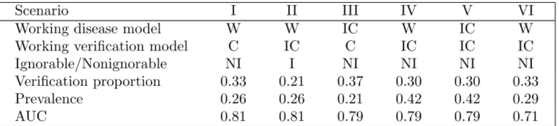
Table 1 summarizes some design statistics for each scenario, including whether the working models are correctly specified, verification proportion, disease preva-lence and the true AUC.
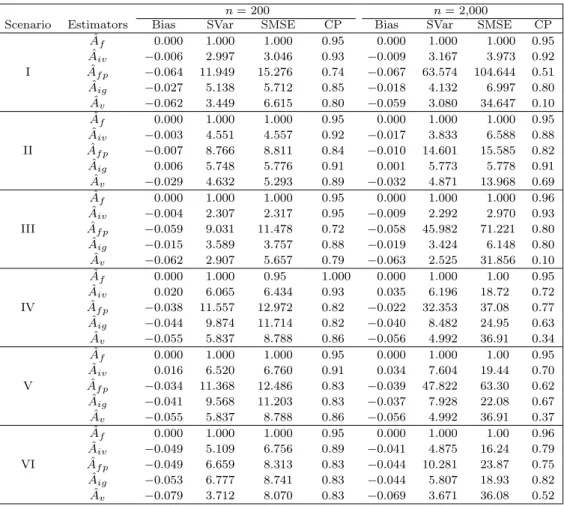
We considered 200 and 2,000 samples for each scenario and generated 500 data sets for each case. Four additional estimators were compared to the proposed estimator: ˆAig, ˆAf, ˆAv and ˆAf p, which stand for the AUC estimators using the
ignorable assumption (β = 0 and without using IV), using full data, using verified data only and using a full parametric disease model (Liu and Zhou (2010)), respectively. We calculated ˆAig and ˆAf pin the same way as ˆAiv, therefore, these
estimators differs in the estimation of parameters φand/or µ.
The estimator ˆAf was treated as the gold standard. A summary of the
simulation results is presented in Table 2, where the bias (defined as the mean difference with ˆAf), standardized sample variance (Svar) and standardized mean
square error (SMSE) are displayed for the six estimators considered. In Table 2, SVar (SMSE) of an estimator is defined as its variance (MSE) divided by the variance (MSE) of ˆAf, and SMSE is also known as relative efficiency. The
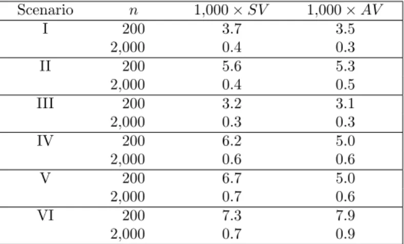
median value of the estimated asymptotic variances for the proposed estimators are compared with the Monte Carlo sample variances in Table 3. The following conclusions can be made from the simulation results.
1. When the verification model is correctly specified (Scenarios I and III), the proposed ˆAiv estimator achieves the best or almost the best performance. Specifically, for nonignorable cases, ˆAiv has the smallest bias and smallest
variance. Also, ˆAiv achieved a closer coverage probability to the nominal level than ˆAv, ˆAig and ˆAf p.
Table 1. Summary statistics for the simulation design. Notation: for working disease model, W – weak misspecification, i.e., disease model is misspecified as having a logistic form, IC – incorrect specification, not only disease model is misspecified as having a logistic form but also the covariates effect misspecified, for working verification model, C – correct specification, the selected instrument variable (IV) is indeed an IV, IC – incorrect specification, indicates that the selected IV is not an IV, I – ignorable scenario, and NI – nonignorable scenario.
Scenario I II III IV V VI
Working disease model W W IC W IC W
Working verification model C IC C IC IC IC
Ignorable/Nonignorable NI I NI NI NI NI
Verification proportion 0.33 0.21 0.37 0.30 0.30 0.33
Prevalence 0.26 0.26 0.21 0.42 0.42 0.29
AUC 0.81 0.81 0.79 0.79 0.79 0.71
2. ˆAiv is robust to the disease model (Scenario III). In the disease model, the
true covariate’s effect is cubic while we fit a linear covariate’s effect. ˆAiv is superior to ˆAv, ˆAig and ˆAf p.
3. When the verification model is incorrectly specified (Scenarios II, IV, V and VI), in the sense of bias or variance, ˆAiv does not always outperform other
estimators, but in the sense of MSE and coverage probability, it outperforms others. Moreover, the proposed estimator generally has similar bias as ˆAf p
but is more efficient than ˆAf p.
4. Further extensive simulation is reported in the supplementary document, including scenarios similar to Scenario III but with different verification proportion and different disease prevalence. The proposed estimator ˆAiv is superior in these studies too.
The asymptotic variance of ˆAiv is compared with its sample variance in Table 3. When the verification model is correct (scenario I and III), the asymptotic variance is very close to the sample variance: When the verification model is in-correctly specified, the asymptotic variance is slightly biased. This indicates that the variance estimation is slightly sensitive to the specification of the verification model.
4.2. Example
We used the Alzheimer’s Disease (AD) data set collected by the National Alzheimer’s Coordinating Center (NACC) to illustrate the proposed method. Liu and Zhou (2010) have analysed an earlier version of this data; the current
Table 2. Monte Carlo bias, standardized variance (SVAR), standardized mean squared error (SMSE) and 95% coverage probability (CP) of AUC estimators in simulation study.
ˆ
Af, ˆAiv, ˆAig, ˆAvand ˆAf pstand for the AUC estimators using full data, using IV method,
using ignorable assumption (missing at random), using verified data only and using a full parametric disease model (Liu and Zhou (2010)), respectively. SVar and SMSE stand for the standardized variance, and standardized MSE, respectively. SVar (SMSE) of an estimator is defined as its variance (MSE) divided by the variance (MSE) of ˆAf. Note
that SMSE is also known as relative efficiency and CP for each AUC estimator was calculated using the median of the sample estimators of the corresponding asymptotic variances.
n= 200 n= 2,000
Scenario Estimators Bias SVar SMSE CP Bias SVar SMSE CP ˆ Af 0.000 1.000 1.000 0.95 0.000 1.000 1.000 0.95 ˆ Aiv −0.006 2.997 3.046 0.93 −0.009 3.167 3.973 0.92 I Aˆf p −0.064 11.949 15.276 0.74 −0.067 63.574 104.644 0.51 ˆ Aig −0.027 5.138 5.712 0.85 −0.018 4.132 6.997 0.80 ˆ Av −0.062 3.449 6.615 0.80 −0.059 3.080 34.647 0.10 ˆ Af 0.000 1.000 1.000 0.95 0.000 1.000 1.000 0.95 ˆ Aiv −0.003 4.551 4.557 0.92 −0.017 3.833 6.588 0.88 II Aˆf p −0.007 8.766 8.811 0.84 −0.010 14.601 15.585 0.82 ˆ Aig 0.006 5.748 5.776 0.91 0.001 5.773 5.778 0.91 ˆ Av −0.029 4.632 5.293 0.89 −0.032 4.871 13.968 0.69 ˆ Af 0.000 1.000 1.000 0.95 0.000 1.000 1.000 0.96 ˆ Aiv −0.004 2.307 2.317 0.95 −0.009 2.292 2.970 0.93 III Aˆf p −0.059 9.031 11.478 0.72 −0.058 45.982 71.221 0.80 ˆ Aig −0.015 3.589 3.757 0.88 −0.019 3.424 6.148 0.80 ˆ Av −0.062 2.907 5.657 0.79 −0.063 2.525 31.856 0.10 ˆ Af 0.000 1.000 0.95 1.000 0.000 1.000 1.00 0.95 ˆ Aiv 0.020 6.065 6.434 0.93 0.035 6.196 18.72 0.72 IV Aˆf p −0.038 11.557 12.972 0.82 −0.022 32.353 37.08 0.77 ˆ Aig −0.044 9.874 11.714 0.82 −0.040 8.482 24.95 0.63 ˆ Av −0.055 5.837 8.788 0.86 −0.056 4.992 36.91 0.34 ˆ Af 0.000 1.000 1.000 0.95 0.000 1.000 1.00 0.95 ˆ Aiv 0.016 6.520 6.760 0.91 0.034 7.604 19.44 0.70 V Aˆf p −0.034 11.368 12.486 0.83 −0.039 47.822 63.30 0.62 ˆ Aig −0.041 9.568 11.203 0.83 −0.037 7.928 22.08 0.67 ˆ Av −0.055 5.837 8.788 0.86 −0.056 4.992 36.91 0.37 ˆ Af 0.000 1.000 1.000 0.95 0.000 1.000 1.00 0.96 ˆ Aiv −0.049 5.109 6.756 0.89 −0.041 4.875 16.24 0.79 VI Aˆf p −0.049 6.659 8.313 0.83 −0.044 10.281 23.87 0.75 ˆ Aig −0.053 6.777 8.741 0.83 −0.044 5.807 18.93 0.82 ˆ Av −0.079 3.712 8.070 0.83 −0.069 3.671 36.08 0.52
data includes the Uniform Data Set (UDS) data up through the September 2014 freeze. Here we want to study the diagnostic ability of the medical test Mini Mental State Examination (MMSE) in detecting AD. MMSE ranges from 0 to 30, with lower scores corresponding to larger risks of having cognitive impairment. The gold standard for AD is based on a primary neuropathological diagnostic test
Table 3. Variance comparison. SV, AV stand for sample variance and the median of estimated asymptotic variance for ˆAiv.
Scenario n 1,000×SV 1,000×AV I 200 3.7 3.5 2,000 0.4 0.3 II 200 5.6 5.3 2,000 0.4 0.5 III 200 3.2 3.1 2,000 0.3 0.3 IV 200 6.2 5.0 2,000 0.6 0.6 V 200 6.7 5.0 2,000 0.7 0.6 VI 200 7.3 7.9 2,000 0.7 0.9
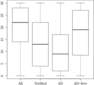
(NPTH), which requires brain autopsy. Some patients or their family do not wish a brain autopsy. These are the main reasons for missing disease status, and only about 10% patients have been verified. Originally, there were several values of NPTH, for example, “Normal”, “definitely AD”, “probably AD”, “possible AD”, etc; we define AD as “definitely AD” (Y = 1) and treat others as control sample (Y = 0). Five covariants, AGE, SEX, marriage status (MRGS), Depression (DEP) and Parkinson’s disease (PD) were considered; these are known to be related to AD or the disease verification. After removing missing values in MMSE and covariants, 52,673 samples remain, in which 5,707 samples were verified by autopsy. In the verified sample, 55% were AD. We also categorized MRGS into two groups; coding “never married” as 1 and the others as 0. The boxplots for MMSE are shown in Figure 1, which shows that lower MMSE scores are more likely to be associated with AD.
We fitted a logistic regression model as the disease model for verified samples: Pr(Yi= 1|Xi, VVVi, Ri = 1) =
1
1 + exp(µ1+µ2Xi+µµµ03VVVi)
, (4.1) whereVVV represents the vector of covariates (AGE, SEX, MRGS, PD, DEP), R
indicates whetherX is observed, andY andXstand for MMSE and true disease status, respectively. The verification model is the logistic regression model
πi = Pr(Ri= 1|Xi, VVVi, Yi) = 1
1 + exp(ψ1+ψ2Xi+ψψψ03VVV1i+βYi)
, (4.2) whereV1are the covariates without the selected IV. For demonstration purposes,
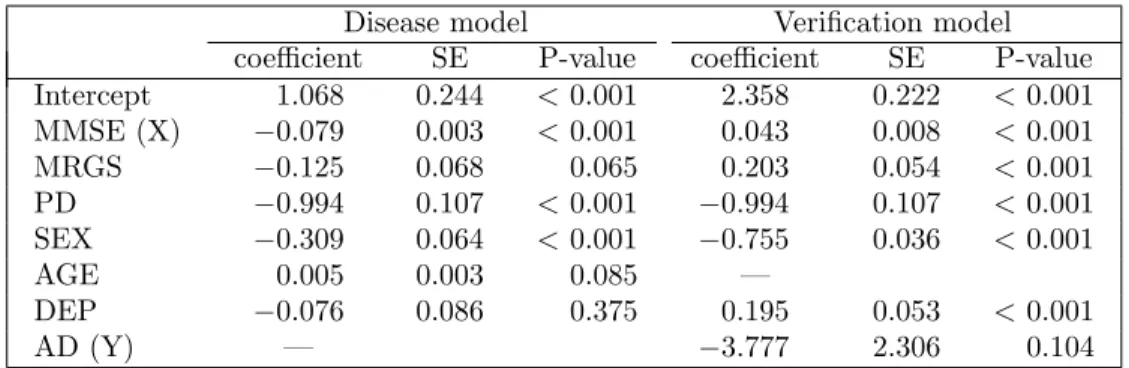
Table 4. Coefficients, Standard error (SE) and p-values.
Disease model Verification model
coefficient SE P-value coefficient SE P-value
Intercept 1.068 0.244 <0.001 2.358 0.222 <0.001 MMSE (X) −0.079 0.003 <0.001 0.043 0.008 <0.001 MRGS −0.125 0.068 0.065 0.203 0.054 <0.001 PD −0.994 0.107 <0.001 −0.994 0.107 <0.001 SEX −0.309 0.064 <0.001 −0.755 0.036 <0.001 AGE 0.005 0.003 0.085 — DEP −0.076 0.086 0.375 0.195 0.053 <0.001 AD (Y) — −3.777 2.306 0.104
covariate vector (MRGS, SEX, PD, DEP). In the Supplementary Material, we extend our study by using different variables as IV. Most of the studies lead to nonsignificantβ or non-convergence, which indicates that there may be no good IV in practice.
The estimated parameters, standard errors and their p-values are listed in Table 4; the p-value was decided by a Wald-statistic and the asymptotic vari-ances calculated according to Lemma 1.1 in the Supplementary Material. All parameters except DEP in the diseased model are significant. The nonignorable parameterβ is estimated to be−3.777 (two-side p-value is about 0.10), which in-dicates that the missing mechanism may be nonignorable. β=−3.777 indicates that the odds of verification for diseased individuals is about exp(3.78) = 43. units larger than it for non-diseased individuals with the same values of (MRGS, SEX, PD, DEP).
The AUC value calculated using only verified samples is 0.699 (95% Con-fidence Interval (CI): 0.686, 0.713), and the proposed estimators ˆAiv = 0.786 (95% CI: 0.754, 0.818). The 95% CIs were constructed using the normal distri-bution. There is a significant difference between our AUC estimators and the AUC calculated only using verified samples (Wald test, p-value < 0.001). The full parametric model in this example is not convergent and, based on our study, using AGE as IV is just for an illustrative example, there may not be good choices of IV here.
5. Concluding Remarks
As it is hard to specify a verification model correctly, sensitivity analyses, as suggested by Rotnitzky, Faraggi and Schisterman (2006), can be used to com-plement the non-robustness. One could also consider nonparametric techniques
"MM 7FSJGJFE "% "%−GSFF
Figure 1. Boxplots for MMSE. “All” – using all samples, “Verified” – using all verified samples, “AD” – using verified AD samples, and “AD-free” – using verified AD-free samples.
such as kernel regression models for the disease model. Bayesian modeling cou-pled with sensitivity analyses in the context of missing data (Daniels and Hogan (2008)) can also be considered for further analyses. This can be a topic of future study.
The proposed method is based on the instrumental variable (IV) assump-tion. We used the variable that had the lowest marginal correlation with R (the verification status) as the IV in our simulation study, which led to good per-formance. This method is not ideal but is simple. Selecting IV is not easy. A good practicable example of IV choice was introduced by Wang, Shao and Kim (2014) for a study of a data set from the Korean Labor and Income Panel Survey (KLIPS). We need more future studies on choosing IV.
After estimating the verification probability and disease probability for each individual, other types of AUC estimators can be used, for example, the other AUC estimators introduced in Alonzo and Pepe (2005) or Liu and Zhou (2010), such as using full imputation (FI) method or mean score imputation (MSI) method instead of inverse probability weighting (IPW) method. The proposed Instrumental Variable method can also be used for FL and MSI. Liu and Zhou (2010) noticed that FI and MSI method generally performed better than the IPW method. One probable reason is that for the IPW method, there are 1/πˆi terms,
and this may produce extreme values for the AUC estimator and its correspond-ing asymptotic variance estimator if the ˆπi are small. In addition to AUC, the
proposed method can be easily extended to the estimation of the other indexes related to ROC curve, such as sensitivity, specificity, and the partial area under the curve (McClish (1989)) as well as the modified area under the Curve (Yu, Chang and Park (2014)).
Supplementary Materials
Supplementary material is available online at http://www3.stat.sinica.edu. tw/statistica/, including proofs of Theorem 3.1, (3.3) and (3.5), and the results from extra numeric studies. The source codes for some of the simulation studies are available on https://github.com/wbaopaul/AUC-IV.
Acknowledgment
The research of Jae Kwang Kim was partially supported by Brain Pool pro-gram (131S-1-3-0476) from the Korean Federation of Science and Technology So-ciety and by a grant from NSF (MMS-1733572). The work of Taesung Park was supported by the Bio & Medical Technology Development Program of the NRF grant (2013M3A9C4078158) and by grants of the Korea Health Technology R & D Project through the Korea Health Industry Development Institute (KHIDI), funded by the Ministry of Health & Welfare, Republic of Korea (HI16C2037, HI15C2165). The NACC database is funded by NIA/NIH Grant U01 AG016976. NACC data are contributed by NIA funded ADCs.
References
Alonzo, T. A. and Pepe, M. S. (2005). Assessing accuracy of a continuous screening test in the presence of verification bias.Journal of the Royal Statistical Society C (Applied Statistics) 54, 173–190.
Baker, S. G. (1995). Evaluating multiple diagnostic tests with partial verification. Biometrics 51, 330–337.
Bamber, D. (1975). The area above the ordinal dominance graph and the area below the receiver operating characteristic graph.Journal of Mathematical Psychology 12(4), 387–415. Begg, C. B. and Greenes, R. A. (1983). Assessment of diagnostic tests when disease verification
is subject to selection bias.Biometrics 39, 207–215.
Daniels, M. J. and Hogan, J. W. (2008).Missing Data in Longitudinal Studies: Strategies for Bayesian Modeling and Sensitivity Analysis. Chapman & Hall / CRC.
receiver operating characteristic curve in the presence of verification bias. Statistics in Medicine 28(3), 361–376.
He, H. and McDermott, M. P. (2011). A robust method using propensity score stratification for correcting verification bias for binary tests.Biostatistics0, 1–15.
Kim, J. K. and Yu, C. L. (2011). A semi-parametric estimation of mean functionals with non-ignorable missing data.Journal of the American Statistical Association 106, 157–165. Kosinski, A. S. and Barnhart, H. X. (2003). Accounting for nonignorable verification bias in
assessment of diagnostic tests.Biometrics 59(1), 163–171.
Liu, D. and Zhou, X.-H. (2010). A model for adjusting for nonignorable verification bias in estimation of the ROC curve and its area with likelihood-based approach. Biometrics 66(4), 1119–1128.
Louis, T. A. (1982). Finding the observed information matrix when using the EM algorithm. Journal of the Royal Statistical Society. Series B (Statistical Methodological) 44, 226–233. McClish, D. K. (1989). Analyzing a portion of the ROC curve.Medical Decision Making 9(3),
190–195.
Riddles, M. K., Kim, J. K. and Im, J. (2016). Propensity-score-adjustment method for nonig-norable nonresponse.Journal of Survey Statistics and Methodology4(2), 215–245. Rodenberg, C. and Zhou, X.-H. (2000). ROC curve estimation when covariates affect the
veri-fication process.Biometrics 56(4), 1256–1262.
Sverchkov, M. (2008). A new approach to estimation of response probabilities when missing data are not missing at random. Proceeding of the Section on Survey Research Methods, 867-874.
Rotnitzky, A., Faraggi, D. and Schisterman, E. (2006). Doubly robust estimation of the area under the receiver-operating characteristic curve in the presence of verification bias.Journal of the American Statistical Association 101(475), 1276–1288.
Wang, S., Shao, J. and Kim, J. K. (2014). An instrumental variable approach for identification and estimation with nonignorable nonresponse.Statistic Sinica24, 1097–1116.
Yu, W., Chang, Y. I. and Park, E. (2014). A modified area under the ROC curve and its application to marker selection and classification.Journal of the Korean Statistical Society 43(2), 161–175.
Zhou, X.-H. (1996). A nonparametric maximum likelihood estimator for the receiver operating characteristic curve area in the presence of verification bias.Biometrics 52, 299–305. Zhou, X.-H. (1998). Comparing correlated areas under the ROC curves of two diagnostic tests
in the presence of verification bias.Biometrics 54, 453–470.
Zhou, X.-H. and Castelluccio, P. (2003). Nonparametric analysis for the ROC areas of two diagnostic tests in the presence of nonignorable verification bias. Journal of Statistical Planning and Inference 115(1), 193–213.
Zhou, X.-H. and Castelluccio, P. (2004). Adjusting for non-ignorable verification bias in clinical studies for alzheimer’s disease.Statistics in Medicine 23(2), 221–230.
Zhou, X.-H., Obuchowski, N. A. and McClish, D. K. (2011).Statistical Methods in Diagnostic Medicine, Volume 712. John Wiley & Sons.
Zhou, X.-H. and Rodenberg, C. A. (1998). Estimating an ROC curve in the presence of non-ignorable verification bias.Communications in Statistics-Theory and Methods 27(3), 635– 657.
Department of Biomedical and Health Informatics, Division of Oncology and Center for Child-hood Cancer Research, Childrens Hospital of Philadelphia, Philadelphia, PA, 19104, USA. E-mail: wbaopaul@gmail.com
Department of Statistics, Iowa State University, Ames, IA 50011, USA. E-mail: jkim@iastate.edul
Department of Statistics, Seoul National University, Shilim-Dong, Kwanak-Gu, Seoul 151-742, Korea.
E-mail: taesungp@gmail.com