Thesis Title
By:
Name of student
A thesis submitted in partial fulfilment of the requirements for the degree of Doctor of Philosophy
The University of Sheffield Faculty of ...
School (or Department) of ....
Submission Date
Sparse Machine Learning Methods for
Autonomous Decision Making
Danil Kuzin
A thesis submitted in partial fulfillment of the requirements for the degree of
Doctor of Philosophy
University of Sheffield 2018
ABSTRACT
Sparse regression methods are used for the reconstruction of compressed signals, that are usually sparse in some bases; or in feature selection problem, where only few features are meaningful. This thesis overviews the existing Bayesian methods for dealing with sparsity, improves them and provides new models for these problems. The novel models decrease complexity, allow to model structure and provide uncertainty distributions in such applications as medicine and computer vision.
The thesis starts with exploring Bayesian sparsity for the problem of compressive back-ground subtraction. Sparsity naturally arises in this problem as foreback-ground usually occupies only small part of the video frame. The use of Bayesian compressive sensing improves the solutions in independent and multi-task scenarios. It also raises an important problem of exploring the structure of the data, as foreground pixels are usually clustered in groups.
The problem of structure modelling in sparse problems is addressed with hierarchical Gaussian processes, that are the Bayesian way of imposing structure without specifying its exact patterns. Full Bayesian inference based on expectation propagation is provided for offline and online algorithms. The experiments demonstrate the applicability of these methods for the compressed background subtraction and brain activity localisation problems.
The majority of sparse Bayesian methods are computationally intensive. This thesis proposes a novel sparse regression method based on the Bayesian neural networks. It makes the prediction operation fast and additionally estimates the uncertainty of predictions, while requiring a longer training phase. The results are demonstrated in the active learning scenario, where the estimated uncertainty is used for experiment design.
Sparse methods are also used as part of other methods such as Gaussian processes that suffer from high computational complexity. The use of active sparse subsets of data improves the performance on large datasets. The thesis proposes a method of dealing with the complexity problem for online data updates using Bayesian filtering.
ACKNOWLEDGMENTS
I would like to thank my supervisor, Prof. Lyudmila Mihaylova for encouragement and guidance of my research. Her insights and knowledge were incredibly inspirational and important during my study. The advices and support kept me on the way to completing this thesis.
I am eternally grateful to my wife, Olga for her help with proofreading of papers and the thesis. Her support with long proofs of some of the methods was enormously helpful. Without the optimism and encouragement from Olga this work would not be possible.
I especially thank my parents, Andrey and Elena, for their financial support during the study. Their moral support was invaluably important for me as well during my life and allowed me to get to this point.
I also acknowledge the support of Seventh Framework Programme TRAcking in compleX sensor systems (TRAX) grant.
CONTENTS
List of Figures ix
List of Tables xi
List of Acronyms xii
List of Notation xiii
Chapter 1: Introduction 1
1.1 Different Forms of Sparsity . . . 1
1.1.1 Compressive Sensing . . . 1
1.1.2 Structural Sparsity . . . 2
1.1.3 Sparse Coding and Supervised Learning . . . 2
1.1.4 Sparse Approximations of Computational Algorithms . . . 2
1.2 Outline and Key Contributions . . . 2
1.3 Disseminated Results . . . 5 Chapter 2: Background 8 2.1 Sparse Regression . . . 8 2.1.1 Frequentist Interpretation . . . 8 2.1.2 Bayesian Interpretation . . . 12 2.2 Compressive Sensing . . . 16 2.2.1 Signal Representation . . . 17 2.2.2 Transform Coding . . . 18 2.2.3 Compressive Sensing . . . 18 2.3 Gaussian Processes . . . 19 2.3.1 Definition . . . 19 2.3.2 Regression . . . 21 v
2.3.3 Classification . . . 22
2.3.4 Scalability . . . 24
2.4 Summary . . . 24
Chapter 3: Compressive Background Subtraction 25 3.1 Background Subtraction . . . 26
3.2 Bayesian Compressive Sensing . . . 27
3.2.1 Multitask Bayesian Compressive Sensing (MTCS) . . . 30
3.2.2 Design matrix selection . . . 30
3.2.3 Complexity . . . 30
3.3 Experiments . . . 31
3.4 Summary . . . 34
Chapter 4: Structured Spike and Slab Models 37 4.1 Group Sparsity . . . 38
4.2 Spike and Slab Models . . . 39
4.2.1 Factor Graphs . . . 40
4.2.2 Spike and Slab Model . . . 40
4.2.3 Spike and Slab Model with a Spatial Structure . . . 41
4.2.4 Gaussian Processes Dynamics System . . . 42
4.3 The Proposed Spatio-temporal Structured Spike and Slab Model . . . 44
4.4 Expectation Propagation for the Hierarchical Spike and Slab Model . . . 46
4.4.1 Expectation Propagation . . . 46
4.4.2 Approximating Factors . . . 48
4.4.3 Full Posterior Approximation . . . 50
4.5 Online Inference with Bayesian Filtering . . . 55
4.5.1 Prediction . . . 55 4.5.2 Update . . . 57 4.5.3 Minibatch Filtering . . . 58 4.5.4 Implementation Details . . . 58 4.6 Experiments . . . 58 4.6.1 Synthetic Data . . . 60
vii
4.6.2 Real Data: Moving Object Detection in Video . . . 62
4.6.3 Real Data: EEG Source Localisation . . . 66
4.6.4 Parameters Selection . . . 67
4.7 Conclusions . . . 68
Chapter 5: Uncertainty Propagation in Sparse Bayesian Neural Networks 71 5.1 Bayesian Neural Networks . . . 72
5.1.1 Sampling Methods . . . 72
5.1.2 Variational Inference . . . 73
5.1.3 Expectation Propagation . . . 73
5.2 Neural Networks for Sparse Coding . . . 73
5.3 Bayesian Neural Network for Sparse Coding . . . 74
5.4 Uncertainty Propagation through Soft-Thresholding . . . 75
5.4.1 Initialisation Dense Layer . . . 75
5.4.2 Soft-Thresholding Nonlinearity . . . 76
5.4.3 Main Layers . . . 77
5.4.4 Bayesian LISTA Forward Propagation . . . 80
5.4.5 Approximation Quality . . . 80 5.5 Backpropagation . . . 81 5.5.1 Likelihood . . . 81 5.5.2 Prior . . . 83 5.5.3 Hyperparameter Optimisation . . . 83 5.6 Experiments . . . 83
5.6.1 Predictive Performance on Synthetic Data . . . 84
5.6.2 Predictive Performance on MNIST Data . . . 85
5.6.3 Active Learning . . . 86
5.7 Summary . . . 87
Chapter 6: Ensemble Kalman Filters for Sparse Gaussian Processes 91 6.1 Sparse Gaussian Processes . . . 92
6.2 Ensemble Kalman Filter Overview . . . 93
6.3.1 Dual Ensemble Kalman Filter for Gaussian Processes . . . 94
6.3.2 Liu-West Filter . . . 97
6.3.3 Computational Complexity of Dual Ensemble Kalman Filter for Gaus-sian Processes . . . 99
6.3.4 Joint Ensemble Kalman Filter for Gaussian Processes . . . 99
6.4 Experiments . . . 100 6.4.1 Synthetic Data . . . 102 6.4.2 House Prices . . . 104 6.5 Summary . . . 106 Chapter 7: Conclusion 108 7.1 Contributions . . . 108
7.2 Directions for Future Work . . . 109
7.2.1 Variational Inference . . . 109
7.2.2 Expectation Propagation . . . 110
7.2.3 Neural Networks Architecture . . . 110
LIST OF FIGURES
2.1 Contour lines example . . . 10
2.2 Graphical models for strong sparsity . . . 15
2.3 DCT transform . . . 17
2.4 CS reconstruction . . . 19
2.5 GP samples . . . 21
2.6 GP regression . . . 22
2.7 GP classification . . . 23
2.8 GP with inducing points . . . 23
3.1 Background subtraction example . . . 26
3.2 Graphical models for BCS . . . 28
3.3 Reconstruction on 2000 measurements . . . 31
3.4 Reconstruction on 5000 measurements . . . 32
3.5 Comparison on 2000 measurements . . . 34
3.6 Comparison on 5000 measurements . . . 35
4.1 Independent spike and slab model . . . 41
4.2 Spatial spike and slab model . . . 43
4.3 Gaussian process dynamic system model . . . 44
4.4 Spatio-temporal spike and slab model . . . 46
4.5 Synthetic data . . . 60
4.6 Synthetic experiment . . . 63
4.7 Background subtraction experiment . . . 64
4.8 Background subtraction reconstructino results . . . 65
4.9 Located dipoles in EEG source localisation . . . 68
4.10 Reconstructed EEG signal . . . 69
4.11 Quality of EEG source localisation . . . 69
5.1 Approximations of Bayesian LISTA . . . 79
5.2 Grid optimisation for the shrinkage parameter λon the synthetic data. . . 84
5.3 Different depth performance . . . 85
5.4 Different observation size performance . . . 86
5.5 Different iteration performance with small dictionary . . . 87
5.6 Different depth performance with large dictionary . . . 88
5.7 Posterior parameters for an image of digit 7 . . . 89
5.8 Samples from the posterior for an image of digit 7 . . . 89
5.9 Performance for the active learning experiment on the MNIST data . . . 90
6.1 Target function and classical GP approximation for the synthetic data . . . . 102
6.2 Performance of the Joint GP-EnKF on the synthetic data . . . 103
6.3 Performance of the Dual GP-EnKF on the synthetic data . . . 104
6.4 Performance of the Liu-West Dual GP-EnKF on the synthetic data . . . 105
6.5 History of quality measures . . . 106
LIST OF TABLES
2.1 Weak sparsity priors represented as the scale mixture of Gaussians . . . 16
3.1 Mean quality measures . . . 36
4.1 Two-level GP hyperparameters . . . 70
6.1 Performance on the synthetic data at N = 200 . . . 104
OMP orthogonal matching pursuit
ISTA iterative shrinkage and thresholding algorithm
LISTA learned iterative shrinkage and thresholding algorithm ADMM alternating direction method of multipliers
GP Gaussian process
BCS Bayesian compressive sensing
MTCS multi-task Bayesian compressive sensing
EP expectation propagation
EEG electroencephalogram
DNN deep neural network
BNN Bayesian neural network
EnKF ensemble Kalman filter NMSE normalised mean square error
LIST OF NOTATION
General notationN number of data points
n index of data point
D dataset K size of observations k index of observation y(n)∈RK n-th observation Y ∈RN×K set of observations D size of coefficients d index of coefficient β(n) ∈RD n-th coefficient B∈RN×D set of coefficients X∈RK×D design matrix ε(n)∈RK n-th noise term σ2 variance of noise
hλ(·) soft thresholding function
I identity matrix δ0(·) delta function Γ(·) gamma function E[·] expectation Var[·] variance Cov[·,·] covariance
Φ(·) standard Gaussian cumulative distribution function (cdf)
N(·) Gaussian distribution
Ber(·) Bernoulli distribution
IG(·) inverse gamma distribution
T(·) Student’st-distribution
Gam(·) gamma distribution Notation specific for Chapter 3
b∈RD background frame
v(n) ∈RD video frame
α precision for prior ofβ(n)
Notation specific for Chapter 4
g(n)(·) factor for distribution of β(n)
σβ2 variance of slab distribution ω(dn) indicator forβ(n)
Ω set of indicators
fd(n)(·,·) factor for distribution of ωd(n),βd(n) γd(n) probability of spike
Γ set of spike probabilities
h(dn)(·,·) factor for distribution of ωd(n),γd(n)
µ(n) mean of the spatial GP
Σ0 covariance of the spatial GP
r(n)(·,·) factor for distribution of γ(n),µ(n)
u(n)(·,·) factor for distribution of µ(n),µ(n−1)
W covariance of the temporal GP
Notation specific for Chapter 5
W LISTA bias matrix
wij element ofW
S LISTA multiplication matrix
xv
cl non-sparse coefficient approximation after layer l
L number of layers
b
βl coefficient approximation after layer l η precision of prior for weights
f(·) output of the Bayesian LISTA neural network
Z normalisation constant
Notation specific for Chapter 6
K number of grid points
g ∈RK mean of the GP
D dimensionality of input
x∈RD domain of the target function
Xg∈RK×D grid points
Lθ number of parameters of the covariance function
θ ∈RLθ parameters of the covariance function
N number of iterations
S number of function observations
y(n)∈RS function observations
Xnew locations of function observation σ2y the variance of noise
η∈RL full vector of algorithm parameters
Chapter 1
INTRODUCTION
Nowadays, massive amounts of data are available for processing. Modern databases contain billions of data entries with thousands of features and, moreover, they are being updated online with more data. It is important to distinguish relevant features for each desired outcome to focus the analysis on them.
The statistical analysis that deals with this problem is usually called variable selection and it is often based on a set of methods called sparse regression. For example, in genetics, variable selection is used to discover genes responsible for diseases from the set of three billion base pairs in the human genome. In electroencephalogram source localisation, the electromagnetic field is measured at a brain cortex and the measurements are used to discover a particular area inside the brain being active at specific activities of a person, which is usually assumed to be small.
1.1 Different Forms of Sparsity
Sparsity appears in many forms and can be used to replicate nature of data or to improve computational complexity.
1.1.1 Compressive Sensing
In the signal processing field, signals are usually represented as linear combinations of basis functions. Real-life periodic signals are generally well approximated in the Fourier basisthat is formed of sines and cosines, typically only a small amount of representation coefficients have large values and others are close to zero. Non-continuous signals or signals with a limited domain can be represented in the wavelet basis, that is a representation of a function by scaled and translated copies of a decaying oscillating waveform. The existence of such
sparse representationsof the real signals allows to reduce the number of samples required to
capture the signal. The area ofcompressive sensing researches ways of optimising sampling rates and it is, again, based on sparse regression methods.
1.1.2 Structural Sparsity
Further research of sparse regression problems leads to the following observation: sometimes genes responsible for deceases are grouped together in a small area of genome; an active brain area for a particular activity is usually small and localised. The knowledge about patterns of meaningful features allows to improve results of sparse regression, such approach is calledstructured sparsity.
1.1.3 Sparse Coding and Supervised Learning
Usually, the problem of sparse regression requires large computational resources for every new data point as the problems are solved independently. A different approach to the problem is based on supervised learning where an algorithm is built to solve sparse regression problems based on a dataset of input and output pairs. For example, a neural network can be trained for sparse regression in this context. It requires significant resources for initial training, but then allows to solve the sparse regression problem for new data efficiently.
1.1.4 Sparse Approximations of Computational Algorithms
The property of sparsity is also an important component of many algorithms. Sparse approximations increase the scalability of Gaussian process regression to larger amounts of data: they allow to select only a small subset of inputs that are most relevant. Sparse matrices of neural network weights may increase the performance of neural networks: they set some of the weights to zeros, thus removing redundant connections.
1.2 Outline and Key Contributions
Overall, this thesis develops machine learning methods for sparse regression, that allow faster, more accurate reconstruction of signals. It also develops sparse modifications of machine learning methods that improve computational requirements. This section provides an outline and key contributions of the thesis.
1.2 Outline and Key Contributions 3
Background
The sparse regression problem is actively researched in statistics with the seminal works of Mitchell and Beauchamp (1988), Tibshirani (1996), Tipping (2001), Gregor and LeCun (2010). These significant developments are presented in Chapter 2 of the thesis.
Compressive Background Subtraction
In Chapter 3 the compressive sensing methods for object detection in video are described and sparse Bayesian models are applied for this problem. They improve the quality results compared to previously existed methods. The main contributions of this chapter are:
Bayesian compressive sensing for background subtraction. The compressive back-ground subtraction problem is for the first time considered within the sparse Bayesian framework and its performance is compared with the existing frequentist methods.
Multitask Bayesian compressive sensing for background subtraction. The multi-task Bayesian framework extends the model for the sequential data that has similar properties.
Structured Spike and Slab Models
Models for structured sparsity are described in details in Chapter 4, and new structured methods that can work without prior knowledge about the exact patterns of sparsity and with online updates of the data are presented there. The key contributions of the chapter are:
Spike and slab model with a hierarchical Gaussian process prior. The model has a flexible structure which is governed only by the covariance functions of the Gaussian processes. This allows to model different types of structures and does not require any specific knowledge about the structure such as determination of particular groups of coefficients with similar behaviour. If, however, there is an information about the structure, it can be easily incorporated into the covariance functions. The model is flexible as spatial and temporal dependencies are decoupled by different levels of the hierarchical Gaussian process prior. Therefore, the spatial and temporal structures are
modelled independently allowing to encode different assumptions for each type of the structure.
Offline inference algorithm. The developed Bayesian inference algorithm based on ex-pectation propagation achieves full posterior inference and perform predictions.
Online inference algorithm. The novel online inference algorithm for streaming data based on Bayesian filtering improves computational time.
Real data applications. A thorough validation and evaluation of the proposed method over synthetic and real data is presented including electrical activity data for the EEG source localisation problem and video data for the compressive background subtraction problem.
Uncertainty Propagation in Sparse Bayesian Neural Networks
In Chapter 5 the sparse regression problem is considered in the context of supervised learning. A novel Bayesian neural network is proposed for sparse regression that combines efficient predictions from neural networks together with uncertainty estimates from Bayesian methods. The main contributions of this chapter are:
Uncertainty propagation for soft-thresholding. In the Bayesian neural network, un-certainty estimation of the predictions can be achieved as a result of sequential weight uncertainty propagation through the layers of a network which leads to complex re-sulting distributions due to nonlinearities involved. To make the posterior inference possible, for the first time a method for uncertainty propagation through the soft thresholding nonlinearity for a Bayesian neural network is proposed, that approximates the resulting distributions with the spike and slab family.
Bayesian LISTA. A posterior inference algorithm for weights and outputs of neural net-works with the soft thresholding nonlinearity is developed. This allows to design a novel Bayesian LISTA neural network for sparse coding.
1.3 Disseminated Results 5
Ensemble Kalman Filters for Sparse Gaussian Processes
In Chapter 6 new methods for sparse approximation of Gaussian processes are presented that use the idea of sequential estimation to operate with online data and they reduce the computational requirements. The main contributions of this chapter can be summarised as:
Gaussian processes with the ensemble Kalman filter method. For the first time the ensemble Kalman filter for the problem of online Gaussian process regression and learn-ing is proposed. The method treats the mean and hyperparameters of the Gaussian process as the state and parameters of the ensemble Kalman filter, respectively. This allows to reduce the computational complexity related to prediction, as the size of the invertible matrices is reduced according to the ensemble sizes. The online evaluation of the parameters and the state is performed on new upcoming samples of data. This procedure iteratively improves the accuracy of parameter estimates. The ensemble Kalman filter reduces the computational complexity required to obtain predictions with Gaussian processes preserving the accuracy level of these predictions.
Dual and joint versions. The dual and joint versions of the ensemble Kalman filter that differently approach the state-parameter relationship are presented in the chapter.
House prices experiments. The performance of the algorithms is compared using the synthetic dataset and real large dataset of the house prices.
Conclusions
Chapter 7 provides an overview of the main results of the thesis and directions for future work based on the methods proposed in the thesis.
1.3 Disseminated Results
The results from this research are disseminated in following papers:
• Danil Kuzin, Olga Isupova, and Lyudmila Mihaylova (2015). “Compressive sensing approaches for autonomous object detection in video sequences”. In: Proceedings of the
Sensor Data Fusion: Trends, Solutions, Applications Workshop (SDF). IEEE, pp. 1–6.
• Danil Kuzin, Olga Isupova, and Lyudmila Mihaylova (2017). “Structured sparse mod-elling with hierarchical GP”. in: Proceedings of the 6th Signal Processing with Adaptive
Sparse Structured Representations Workshop (SPARS).url: http://spars2017.lx.
it.pt/index_files/papers/SPARS2017_Paper_48.pdf
• Danil Kuzin, Le Yang, Olga Isupova, and Lyudmila Mihaylova (2018). “Ensemble Kalman filtering for online Gaussian process regression and learning”. In: Proceedings
of the 21st International Conference on Information Fusion (FUSION). IEEE, pp. 39–
46. doi: 10.23919/ICIF.2018.8455785
• Danil Kuzin, Olga Isupova, and Lyudmila Mihaylova (2018a). “Spatio-temporal structured sparse regression with hierarchical Gaussian process priors”. In: IEEE
Transactions on Signal Processing vol. 66, issue 17, pp. 4598–4611. doi: 10.1109/
TSP.2018.2858207
• Danil Kuzin, Olga Isupova, and Lyudmila Mihaylova (2018b). “Uncertainty propa-gation in neural networks for sparse coding”. In: Proceedings of the Third Workshop
on Bayesian Deep Learning (NeurIPS).url: http://bayesiandeeplearning.org/
2018/papers/47.pdf
• Danil Kuzin, Olga Isupova, and Lyudmila Mihaylova (2019). “Bayesian neural networks for sparse coding”. Accepted at IEEE International Conference on Acoustics, Speech and Signal Processing (ICASSP)
Other co-authored works during my study at the University are:
• Olga Isupova, Danil Kuzin, and Lyudmila Mihaylova (2015). “Abnormal behaviour detection in video using topic modeling”. In: USES Conference Proceedings. The University of Sheffield. doi: 10.15445/02012015.18
• Olga Isupova, Lyudmila Mihaylova, Danil Kuzin, Garik Markarian, and Francois Septier (2015). “An expectation maximisation algorithm for behaviour analysis in video”. In:
Proceedings of the 18th International Conference on Information Fusion (FUSION).
IEEE, pp. 126–133. url: https://ieeexplore.ieee.org/document/7266553/
• Olga Isupova, Danil Kuzin, and Lyudmila Mihaylova (2016). “Dynamic hierarchical Dirichlet process for abnormal behaviour detection in video”. In: Proceedings of the
1.3 Disseminated Results 7
19th International Conference on Information Fusion (FUSION). IEEE, pp. 750–757.
url: https://ieeexplore.ieee.org/document/7527962/
• Olga Isupova, Danil Kuzin, and Lyudmila Mihaylova (2018). “Learning methods for dynamic topic modeling in automated behavior analysis”. In: IEEE Transactions
on Neural Networks and Learning Systems vol. 29, issue 9, pp. 3980–3993. issn:
BACKGROUND
This chapter presents the sparse regression problem and important solutions for it that lay the foundation of the thesis. It also describes the compressive sensing problem that is used in most experiments throughout the thesis. In addition, it overviews a Gaussian process which is the significant part of the methodology in the thesis.
2.1 Sparse Regression
The main goal of sparse regression is to recover the coefficient vectors based on the observed
vectorsand the design matrix with the assumption of sparsity of the coefficient vectors. The
prevalent form of relationship between coefficients and observations is linear, as this degree of freedom is enough for many real-world applications. It can be achieved with a linear regression approach.
Let the data be represented byN observations asD={y(n),β(n)}N
n=1. Every observation
nconsists of the coefficient vectorβ(n)∈RD and the observed vector y(n) ∈
RK. The linear
relationship is represented using the design matrixX∈RK×D of covariates as
y(n)=Xβ(n)+ε(n), (2.1)
whereε(n)∈RK is the noise that captures other factors not included in the linear model.
The sparsity assumption can be expressed with penalty constraints in the frequentist interpretation of statistical inference, or priors in the Bayesian interpretation.
2.1.1 Frequentist Interpretation
In thefrequentist statistics the coefficients β(n) are fixed and unknown, they are selected so
that the resulting distribution ony(n) matches the real distribution for training data.
2.1 Sparse Regression 9
The frequentist interpretation of sparsity is to solve a regularised regression problem. For example, lp–norm penalty functions with 0< p <2 encourage sparse solutions of the
coefficient vector: β(n)=argminβ(n) h ||y(n)−Xβ(n)||22+||β(n)||ppi, (2.2) wherelp norm is ||β(n)||p = D X d=1 |βd(n)|p !1p . (2.3)
As papproaches zero, the penalty function becomes the function that counts the number of
non-zero elements of the coefficient vector, which could be interpreted as the true sparsity penalty for many problems.
For the intuition, whylp-penalty functions provide sparse solutions, Figure 2.1
demon-strates an example of two-dimensional contour lines for the error term ||y(n)−Xβ(n)|| 2 and the penalty term ||β(n)||p for different p. For sparsity-inducingp, the sum of these terms is
minimal when the solution is sparse.
Different choices ofpin these penalty functions provide solutions with different properties,
that are further discussed. While there exist a great amount of algorithms for different frequentist interpretations of sparsity (Bach et al. 2012a), this section presents only the examples that are used in the thesis.
Regularisation with Non-zero Counting Penalty
The non-zero counting penalty function (p→0) is the most obvious approach for sparsity,
but the solution of such optimisation problem is NP-hard (Bach et al. 2012a). The globally optimal solution can be found only by comparing the target function for all possible values of coefficients, that is computationally intensive. Greedy algorithms, such as matching pursuits (Mallat and Zhang 1993), are used for this problem, however, they tend to find only locally optimal solutions.
Consider the problem (2.2) for one data pointn. Orthogonal matching pursuit (OMP) is
a greedy method that iteratively updates the set γ of the non-zero elements ofβ(n). Initially,
3 2 1 0 1 2 3 2.0 1.5 1.0 0.5 0.0 0.5 1.0 1.5 2.0 (a)l2-ball 3 2 1 0 1 2 3 2.0 1.5 1.0 0.5 0.0 0.5 1.0 1.5 2.0 (b) l1-ball 3 2 1 0 1 2 3 2.0 1.5 1.0 0.5 0.0 0.5 1.0 1.5 2.0 (c)l1/2-ball 3 2 1 0 1 2 3 2.0 1.5 1.0 0.5 0.0 0.5 1.0 1.5 2.0 (d) l1/8-ball
Figure 2.1: Example contour lines for different values ofp. Red lines are the contour lines for
the error term, with minimum atβ(n)= (1.5,1.0). Blue lines are the contour lines for the
penalty term, with minimum atβ(n)= (0,0). The minimal sum of these terms is displayed
as a point, one of which components moves towards zero asp approaches zero, therefore
2.1 Sparse Regression 11
d∗ as the most correlated with the current residual and not included in the active set yet d∗ = argmin d6∈γ n min ω ||y (n)−Xβ(n) l −ωx:,d||2 o , (2.4)
wherex:,d denotes thed-th column ofX. The inner optimisation is solved as ω= x > :,drl ||x:,d||22 , (2.5) withrl =||y(n)−Xβ (n)
l ||2 being the current residual.
Regularisation with lp-quasinorm, 0< p <1
For 0< p <1, the penalty term (2.3) is non-convex. While, in theory, these penalties may
provide better results than the l1 penalty and be more computationally efficient than the non-zero counting penalty, there are no optimisation methods developed for these penalties. The recent piece-wise quadratic error potentials method (Gorban et al. 2016) is an attempt to tackle this problem, however, it is not well-researched yet and is out of scope for this thesis.
Regularisation with l1-norm
For p = 1, the problem (2.2) is called lasso (Tibshirani 1996). The penalty function is
convex, but non-smooth. The convexity of the problem allows to use general efficient convex optimisation methods to find optimums.
Iterative shrinkage and thresholding algorithm (ISTA) (Daubechies et al. 2004) iteratively obtains the new approximation of the coefficient vector [βb
(n)
]l at the iteration l as the
linear transformation of the inputy(n) with the previous approximation [βb (n)
]l−1 and then propagates the new approximation through the soft thresholding function hλ(·)
hλ(v) =sgn(v) max(|v| −λ,0), (2.6)
whereλis a shrinkage parameter. The linear transformation is
b
β(ln)=Wy(n)+Sβb (n)
l−1, (2.7)
with weights W =X>/E, E — the upper bound on the largest eigenvalue of X>X and S=ID×D −WX,ID×D is the identity matrix of size D.
Alternating direction method of multipliers (ADMM) is the general-purpose algo-rithm that can solve the convexl1 optimisation problem using the augmented Lagrangian scheme (Boyd et al. 2011). It augments the problem with an additional variable c, and weightsγ,ρ, and Λ
L= 0.5||y(n)−Xβ(n)||2
2+γ||c||1+ 0.5ρ||β(n)−c||22+Λ(β(n)−c), (2.8) and minimises the Lagrangian sequentially w.r.t. to the targetβ(n) and augmented variable
c thus solving two less complex optimisation problems: the least-square regression and independent one-dimensionall1 minimisation that has soft thresholding as a solution.
Regularisation with lp-norm,1< p <2
When1< p <2, the penalty term is convex and smooth. An example is the elastic net (Zou
and Hastie 2005). Smooth penalty function allows to use more efficient gradient-based techniques, but solutions are less sparse then in the previous cases.
2.1.2 Bayesian Interpretation
In the Bayesian interpretation, the distribution of noise is assumed Gaussian, ε(n) ∼ N(0, σ2I), and distribution of coefficients β(n) and noise varianceσ are assumed unknown.
A prior distribution of coefficients is used to update a posterior distribution of the coefficients based on the likelihood of the observed data. The posterior distribution is estimated using the Bayes rule
p(β(n), σ|y(n)) = p(y
(n)|β(n), σ)p(β(n), σ) R
p(y(n)|β(n), σ)p(β(n), σ)dβ(n)dσ. (2.9) The prior term p(β(n), σ) has been extensively studied in the literature to find an optimal
representation of the prior knowledge. In this chapter the solutions leading to sparse posterior estimates ofβ(n) are considered.
The main difficulty in the Bayesian approach is evaluation of the integral in (2.9). In order to make it tractable,conjugacy is used: given thelikelihood p(y(n)|β(n), σ), theprior p(β(n), σ) is usually selected in the way that the posterior p(β(n), σ|y(n)) lies in the same class of distributions as the prior. The examples are: the beta likelihood with the binomial prior, the multinomial likelihood with the Dirichlet prior, or the Gaussian likelihood with the Gaussian-inverse-Wishart prior. All these distributions belong to theexponential family.
2.1 Sparse Regression 13
In most cases the integral in (2.9) is intractable. This leads to a great amount of inference techniques proposed in the literature. A general overview of inference methods is given by Bishop (2006), Koller and Friedman (2009), and Murphy (2012).
The Bayesian models for sparse regression can be classified into the models withweak
sparsity prior and strong sparsity prior. The weak sparsity prior is a unimodal distribution
of the coefficient vector with a sharp peak at zero. The strong sparsity prior is a mixture of latent binary variables that capture whether a coefficient is zero or not.
Strong Sparsity
The two important strong sparsity prior models are the spike and slab model and the
Bernoulli–Gaussian model. These models put the discrete probability of being zero on each
coefficient.
In the first spike and slab formulation (Mitchell and Beauchamp 1988) each component of β(n) is selected from a mixture of a spike, that is the delta-function in zero, and a slab,
that is the uniform distribution with width 2a:
βd(n)|ω∼
{0}, with the probabilityω;
U[−a;a]\ {0}, with the probability1−ω.
(2.10) Sparsity naturally comes from the prior formulation as the coefficients are exactly zeros with the predefined probability ω. This sparsity representation has been further developed by
utilising different distributions for slabs.
The spike and slab model can be represented in terms of mixtures of Gaussian distribu-tions (George and McCulloch 1993)
βd(n)|ωd, τd, cd∼ωdN(βd(n); 0, τd2) + (1−ωd)N(βd(n); 0, c2dτd2). (2.11)
In this model the spike is a narrow Gaussian distribution with the variance τd, while the
slab is a wide Gaussian distribution, where the variance is cdτd.
Following the Bayesian approach, hidden variableszd(n) that are indicators of spikes are
inverse gamma distributions are placed over the model varianceσβ2 (Murphy 2012)
βd(n)|zd(n), σ2β ∼(1−zd(n))N(βd(n); 0, σβ2) +zd(n)δ0, (2.12a)
zd(n)|ω ∼Ber(zd(n);ω), (2.12b) σ2|aσ, bσ ∼IG(σ2;aσ, bσ). (2.12c)
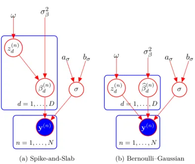
The graphical model for such spike and slab formulation can be found in Figure 2.2a. The Bernoulli-Gaussian model is also widely considered (Soussen et al. 2011; Zhou et al. 2009). Coefficients are presented as a pair-wise product of
β(n)=z(n)◦βb (n) , (2.13a) zd(n)|ω∼Ber(zd(n);ω), (2.13b) b βd(n)|σβ2 ∼ N(βb (n) d ; 0, σ 2 β), (2.13c) σ2|aσ, bσ ∼IG(σ2;aσ, bσ). (2.13d)
The model is different from the spike and slab formulation in the sense of a hierarchy between coefficients and latent variables. This can be seen from graphical model in Figure 2.2b. Inference
The most popular inference schemes for these models aresampling methods (Chipman et al. 2001). In addition, the message passing algorithms can be used: approximate message
passing(Donoho et al. 2009) andexpectation propagation (Lobato,
Hernández-Lobato, et al. 2015). The advantage of the Bernoulli–Gaussian formulation is that it allows to implement the mean-field variational inference (Titsias and Lázaro-Gredilla 2011). Weak Sparsity
The weak sparsity prior models are the other class of priors for sparse Bayesian regression. Many exponential family distributions can be represented as a ratio of two independent variables, where the denominator has the standard Gaussian distribution (Andrews and Mallows 1974). These models, that are calledscale mixtures of Gaussians, allow to create symmetrical unimodal distributions that are peaked in zero and have heavy tails.
2.1 Sparse Regression 15 y(n) βd(n) σ zd(n) ω σβ2 aσ bσ d= 1, . . . , D n= 1, . . . , N (a) Spike-and-Slab y(n) b βd(n) σ zd(n) ω σβ2 aσ bσ d= 1, . . . , D n= 1, . . . , N (b) Bernoulli–Gaussian
Figure 2.2: Graphical models for the sparse regression problem. In the spike and slab model (a) latent variables {zd(n), β(dn)}are organised in hierarchy and the indicators of spikes
zd(n) can be integrated out. In the Bernoulli-Gaussian model (b) the product z(dn)βb (n)
d always
exists.
Scale mixtures of Gaussians can be represented as a hierarchical model:
β(n)|µ,Σ∼ N(β(n);µ,Σ), (2.14)
µ,Σ|τ ∼ψ(µ,Σ;υ). (2.15)
whereψ is the mixing distribution parameterised byυ, which may vary in different models.
Marginalisation of the parameters of the Gaussian distribution leads to
p(β(n)|υ) =
Z
N(β(n);µ,Σ)ψ(µ,Σ;υ)dµdΣ. (2.16)
For sparse priors,µ is set to a zero vector to ensure that the distributions have a peak
exactly at this point.
scale mixtures of Gaussians can be used (Polson and Scott 2010):
βd(n)|τ, λd∼ N(βd(n); 0, τ λd), (2.17)
λd∼π(λd), (2.18)
τ|σ∼φ(τ;σ), (2.19)
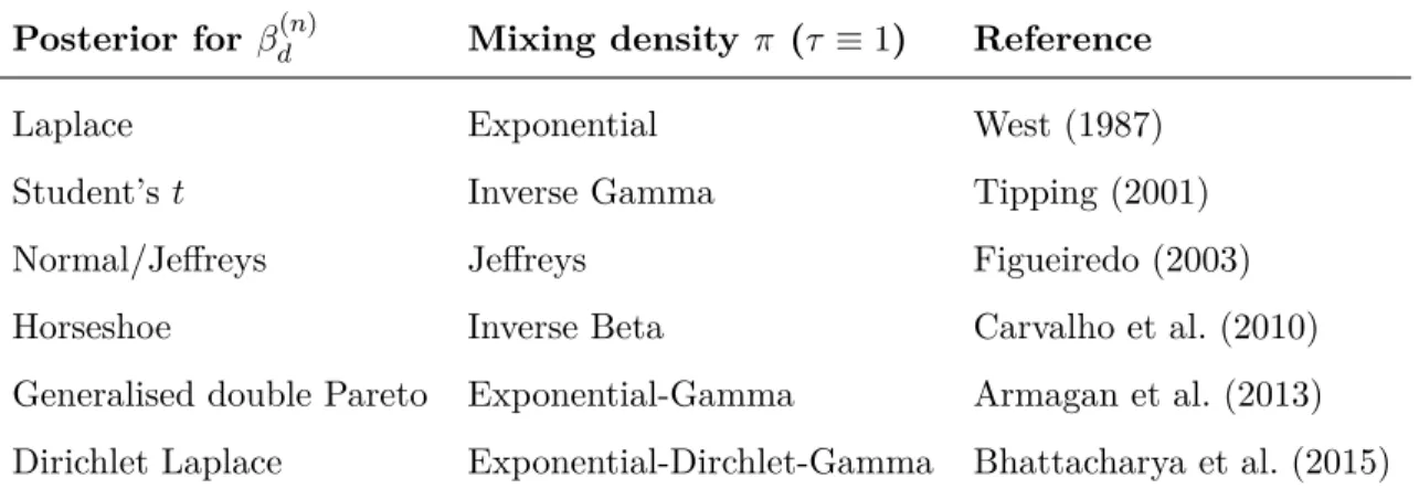
whereπ andφare priors for the local varianceλand global variance τ, respectively. Many
of the existing sparse priors have this representation. They are summarised in Table 2.1
Posterior for β(dn) Mixing density π (τ ≡1) Reference
Laplace Exponential West (1987)
Student’st Inverse Gamma Tipping (2001)
Normal/Jeffreys Jeffreys Figueiredo (2003)
Horseshoe Inverse Beta Carvalho et al. (2010)
Generalised double Pareto Exponential-Gamma Armagan et al. (2013) Dirichlet Laplace Exponential-Dirchlet-Gamma Bhattacharya et al. (2015)
Table 2.1: Weak sparsity priors represented as the scale mixture of Gaussians
Laplace and Student’stpriors are very popular in the literature and different approaches
to inference have been proposed: Gibbs sampling (Hans 2009; Park and Casella 2008), expectation propagation (Seeger 2008), variational inference (Armagan 2009), double-loop algorithm (Seeger and Nickisch 2011) and expectation maximisation (Tipping and Faul 2003).
The Horseshoe density has the infinite spike at zero and heavy tails (Carvalho et al. 2010). This leads to better sparse recovery (Bhattacharya et al. 2015; Polson and Scott 2010).
2.2 Compressive Sensing
Signal acquisition and compression are important areas in signal processing. The compressed information can be used to reconstruct the original signal and for its analysis. Thecompressive
2.2 Compressive Sensing 17 4600 4800 5000 5200 5400 time, ms −3000 −2000 −1000 0 1000 2000 3000 am pli tud e
(a) Part of the signal
0 200 400 600 800 1000 frequency −40000 −20000 0 20000 40000 60000 80000 100000 DC T co eff ic ie nt s
(b) First coefficients of DCT transform
Figure 2.3: Example signal and its DCT transform. It can be noted that after this transform, the resulting coefficients are sparse, as there are only few dominating frequencies.
to reduce the number of measurements required for the ideal reconstruction of the signal. Compression is achieved utilising sparse representations of the signals in preselected basis. 2.2.1 Signal Representation
In signal processing signals are usually represented in bases. If the vectors {ψd}D
d=1 form an orthonormal basis ofRD then any signalθ(n) ∈RD from the set of signalsΘ={θ(1). . .θ(N)}
can be represented in the form
θ(n) = D
X
d=1
β(dn)ψd, (2.20)
where basis coefficientsβ(dn) =hθ(n),ψdi=PD
l=1θ (n)
l ψld are projections of the signal onto
the basis vectors. Consider matrix Ψ:= [ψ1. . .ψD]. The representation of the signal can
be written as
θ(n)=Ψβ(n). (2.21)
Often, signals can be represented in the Fourier-related basis, that is a sum of sinusoidal functions with scaled amplitudes. It can be achieved with, for example, a discrete cosine transform (DCT). Figure 2.3 demonstrates the transform of the sample signal with DCT.
For signals with discontinuities, Fourier coefficients become oscillating and, therefore,β(n)
Mallat 2008) are another important example of bases that better approximate non-smooth or localised signals. They usually achieve sparse representation in image compression. 2.2.2 Transform Coding
The information about sparse representation is used for compressing signals. One of the examples of the algorithms for compression is calledtransform coding(Baraniuk, Cevher, et al. 2010). It is used in MPEG and JPEG formats for media compression. The algorithm consists of the following steps:
1. acquire the full signalθ(n);
2. compute set of basis coefficientsβ(n)=Ψ−1θ(n);
3. locateS largest coefficients and discard others, whereS is the sparsity of the signal;
4. encode locations and values of the largest coefficients.
Then the original signal can be reconstructed from this information. 2.2.3 Compressive Sensing
Compressive sensing (Candes, Romberg, et al. 2006; Donoho 2006) integrates the acquisition
and compression steps and allows to reconstruct the original signal from less measurements and without the information of coefficient locations compared to transform coding. This includes two components: random projections and information that the signal is sparse in some basis.
Assume that the signal θ(n) is not observed directly and only the random projections
y(n) of the signal are aquired
y(n) =Aθ(n). (2.22)
Here matrixAis the random projections matrix that produces a linear transformation of the signal, which is less in dimensionality that the original signal. The signalθ(n) can’t be
restored directly from the measurements, therefore the additional assumption of sparsity is used (2.21). The resulting problem is
2.3 Gaussian Processes 19 0 200 400 600 800 1000 frequency −40000 −20000 0 20000 40000 60000 80000 100000 DC T co eff ic ie nt s true reconstructed (a) DCT coefficients 4600 4800 5000 5200 5400 time, ms −3000 −2000 −1000 0 1000 2000 3000 am pli tud e true reconstructed (b) Signal
Figure 2.4: Reconstruction after compressive sensing. Matrix A is used to generate random projections with size10% of the signal. MatrixΨis the inverse DCT operator.
whereβ(n) is a sparse vector. This prior information is used to regularise the problem and
find a unique solutionβ(n) and, therefore, restore the signalθ(n). The reconstruction results
for the previously considered sample signal are presented in Figure 2.4.
Usually, the components of the matrix Aare sampled from the independent Gaussian distributions, but in general it can be any matrix, which is close to orthonormal1.
2.3 Gaussian Processes
Gaussian process (GP) is one of the Bayesian approaches for placing a prior distribution over the space of functions. This is a broad area that has different applications: latent variable models (Damianou et al. 2016) that are used for non-linear dimensionality reduction, Bayesian optimization (Brochu et al. 2010) that is used for black-box optimisation of unknown functions, and spatio-temporal modelling (Sarkka et al. 2013).
2.3.1 Definition
In probability theory, random variables are sometimes represented in collections. A collection of random variables indexed by set T is called stochastic processξ(t), t∈ T. Index sets can 1The measure of how close the matrix is to orthonormal is derived with restricted isometry property (Candes
represent time, space, or more general concepts.
Gaussian processf(t) is a stochastic process, such that for every finite subset of indices
T = {t(1), . . . ,t(N)} ∈ T values f = {f(t(1)), . . . , f(t(N))} have a multivariate Gaussian distribution with a meanµand covariance matrix Σ
p(f) =N(f;µ,Σ). (2.24)
The mean and covariance for subsets of indices are generalised into the mean and covariance functions of the GP
• Mean function
m(t) =Ef(t). (2.25)
• Covariance function
k(t(n0),t(n00)) =cov(f(t(n0)), f(t(n00))). (2.26)
With the mean and covariance functions, the mean and covariance matrix for the subset of indices are µ= m(t(1)) . . . m(t(N)) , Σ= k(t(1),t(1)) . . . k(t(1),t(N)) . . . . k(t(N),t(1)) . . . k(t(N),t(N)) . (2.27)
Mean and covariance functions completely define a GP. Different covariance function families characterise smoothness and stationarity of a GP.
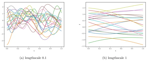
An example of an infinitely smooth covariance function is the squared exponential function
k(t(n0),t(n00)) =σ2exp ( X k (t(kn0)−t(kn00))2 lk ) , (2.28)
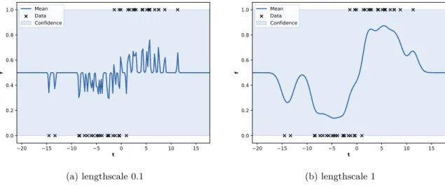
whereσ2 is the variance parameter,lis the vector of lengthscale parameters. The example of samples from a GP with the squared exponential function is demonstrated in Figure 2.52
2.3 Gaussian Processes 21 0.0 0.2 0.4 0.6 0.8 1.0 t −3 −2 −1 0 1 2 f (a) lengthscale 0.1 0.0 0.2 0.4 0.6 0.8 1.0 t −1.5 −1.0 −0.5 0.0 0.5 1.0 1.5 f (b) lengthscale 1
Figure 2.5: Samples from the GP with the squared exponential covariance function. This covariance function provides very smooth samples with different length-scales.
2.3.2 Regression
One of the basic machine learning problems solved with GPs is regression: predict unknown function values at the test points t∗ based on known function values at the training data points {t(n), y(n)}N
n=1. Usually observations are corrupted with noise
y(n)=f(t(n)) +ε(n), ε(n)∼ N(0, σ2). (2.29)
Denote y = [y(1), . . . , y(N)]. In case of the Gaussian noise, p(f(t∗)|y) is a conditional
Gaussian distribution and it is possible to analytically compute predictions
p(f(t∗)|y) =
Z
p(f(t∗)|f)p(f|y)df. (2.30)
In this equation, all distributions are Gaussian, therefore predictions are also Gaussian
f(t∗|y)∼ N(µ∗,Σ∗). (2.31)
The parameters of this distribution are computed based on the properties of Gaussian distributions. Denote T= [t(1), . . . ,t(N)], then
µ∗=k(t∗,T)[k(T,T) +σ2I]−1y, (2.32a)
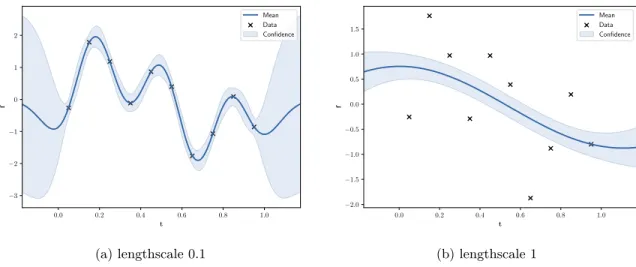
0.0 0.2 0.4 0.6 0.8 1.0 t −3 −2 −1 0 1 2 f Mean Data Confidence (a) lengthscale 0.1 0.0 0.2 0.4 0.6 0.8 1.0 t −2.0 −1.5 −1.0 −0.5 0.0 0.5 1.0 1.5 f Mean Data Confidence (b) lengthscale 1
Figure 2.6: Predictions of Gaussian process regression. For every point, its predicted mean and variance can be computed.
Parameters of the covariance function can be optimised by maximising the likelihood of the observations p(y|t(1), . . . ,t(N)), however, this optimisation may converge to local extrema. An example of GP regression is provided in Figure 2.6.
2.3.3 Classification
Another basic machine learning problem is two-class classification: map test data into one of two classesy∈ {0,+1}, based on known classes for train data {t(n), y(n)}N
n=1. The relationship between observations and class labels is non-linear, it can be represented with, for example, the logistic function
y(n)= 1
1 + exp(−f(t(n)) +ε(n)), (2.33) that outputs values in the interval(0,1).
The likelihood function is not Gaussian, and this integral cannot be analytically computed
p(f(t∗)|y) =
Z
p(f(t∗)|f)p(f|y)df. (2.34)
The same problem holds for all types of non-linear functions that can be used for classifica-tion. Different approaches were proposed for this problem, such as numerical integration,
2.3 Gaussian Processes 23 20 15 10 5 0 5 10 15 t 0.0 0.2 0.4 0.6 0.8 1.0 f Mean Data Confidence (a) lengthscale 0.1 20 15 10 5 0 5 10 15 t 0.0 0.2 0.4 0.6 0.8 1.0 f Mean Data Confidence (b) lengthscale 1
Figure 2.7: GP classification. The class label {0,1}is predicted based on the distribution of the latent function at the corresponding point.
sampling methods (Markov chain Monte Carlo), approximate Bayesian inference (expectation propagation, variational inference, Laplace approximation).
An example of GP classification is presented in Figure 2.7.
2 0 2 4 6 8 10 12 t 2 1 0 1 f Mean Inducing Confidence
(a) Sparse predictions with randomly selected inducing points 2 0 2 4 6 8 10 12 t 4 3 2 1 0 1 2 3 4 f Mean Confidence (b) Full GP prediction
Figure 2.8: Inducing points for Gaussian process regression. A subset of training data was used for predictions. The locations of inducing points can be optimised for better predictions.
2.3.4 Scalability
All operations with GPs require inverting a matrix of sizeN×N, whereN is the number of
training data points. This hasO(N3)computational complexity and requiresO(N2)storage,
which limits the application of GPs to large datasets.
Currently, there is an ongoing work to reduce the computational and memory complexities, which is mostly based on the idea of sparse approximations: choose a small active subset of data points, called inducing points, that give similar prediction results to the whole training dataset.
An example of inducing points for GPs is presented in Figure 2.8
2.4 Summary
This chapter provides on overview of relevant sparse methods. First, the sparse linear regression problem is introduced with the frequentist and Bayesian approaches. Then, the overview of sparse representation in signal processing is described. Finally, sparsity in Gaussian processes is presented.
Chapter 3
COMPRESSIVE BACKGROUND
SUBTRACTION
Sparse models are actively applied for image and video processing (Mairal, Bach, and Ponce 2014). One of the essential problems in video processing is background subtraction, that is detection of changes in sequential video frames. This is important for object localisation and classification, which can be used, for example, for gesture recognition or traffic monitoring. Sparsity is natural for the background subtraction problem, as the foreground objects occupy the small regions on a frame. Background subtraction hence represents a natural application area for sparse modelling. The idea to apply compressive sensing for background subtraction is originally proposed by Cevher et al. (2008), where the sparse regression problem is formulated as the optimisation problem with l1-optimisation.
The Bayesian approach for compressive sensing (Ji, Xue, et al. 2008) provides two desirable properties for the solution: first, it naturally provides the uncertainty estimation of the predictions from the posterior distribution; second, it allows to use adaptive approach for design matrix selection, thus improving efficiency of compression. In this chapter the sparse Bayesian models are considered for compressed background subtraction. As it is shown in the experiments section, they also achieve better computational time.
The chapter is organised as following. In Section 3.1 the sparse model of background subtraction is explained. The Bayesian compressive sensing approaches for this problem is presented in Section 3.2. The experimental results are presented in Section 3.3. Section 3.4 summarises the chapter.
The materials of this chapter were published as
• Danil Kuzin, Olga Isupova, and Lyudmila Mihaylova (2015). “Compressive sensing approaches for autonomous object detection in video sequences”. In: Proceedings of the
(a) Background frame (b) Frame with object (c) Foreground mask
Figure 3.1: Example of background subtraction problem: extract foreground car silhouette from the image. For static camera foreground is sparse, as it occupies only small part of the image.
Sensor Data Fusion: Trends, Solutions, Applications Workshop (SDF). IEEE, pp. 1–6.
doi: 10.1109/SDF.2015.7347706
3.1 Background Subtraction
In a typical background subtraction application the data consists of the sequential frames V(n) ∈RD1×D2, n ∈ {1, . . . , N} from the camera. Assume that the camera is static and
it is possible to acquire a frame B ∈ RD1×D2 from the camera that is referenced as the
background. The problem is to estimate the mask of the foreground objects in the camera frames. The example of camera frames is presented in Figure 3.1.
To preprocess the video, the camera frames are converted to greyscale and flattened: the resulting background frame is vectorb∈RD, the video frames are vectorsv(n)∈
RD, where
D=D1D2.
Usually the foreground objects take only a part of the image, therefore the majority of the foreground maskβ(n)=v(n)−bvalues are close to zero. This leads to the application of sparse regression and compressive sensing theory to this problem. They reduce the number of measurements that need to be taken (Candès and Wakin 2008) and also the results may be denoised (Mairal, Bach, and Ponce 2014). The values of the foreground mask are estimated
3.2 Bayesian Compressive Sensing 27
based on the set of the compressed measurements y(n)∈RK
y(n) =Xβ(n), (3.1)
where the design matrixX∈RK×D consists of i.i.d. Gaussian variables, according to Bara-niuk, Davenport, et al. (2008).
Sinceβ(n)=v(n)−b, the estimates of the coefficientsy(n)can be done on the acquisition step as
y(n)=Xv(n)−Xb. (3.2)
The vectors Xband Xv(n) are the linear combinations of the pixels of the video frames, and a single pixel camera (Duarte et al. 2008) may be used for simultaneous capturing and compression of the video.
In this chapter the Bayesian weak sparsity models for sparse regression are used for the background subtraction problem and their performance is compared with OMP (Sec-tion 2.1.1).
3.2 Bayesian Compressive Sensing
Model
In Bayesian compressive sensing (BCS), the system (3.1) is reformulated as a linear regression model (Ji, Xue, et al. 2008)
y(n)=Xβ(n)+ε(n), (3.3)
whereε(n)is a vector which elements are the independent noise from the Gaussian distribution
ε(dn)∼ N(0, σ2) with the varianceσ2. Therefore, the likelihood can be expressed as
p(y(n)|β(n), σ2) = K
Y
k=1
N(yk(n);xk,:β(n), σ2I), (3.4) wherexk,:is the k-th row of the matrix X.
To implement the full Bayesian approach, the prior distributions are imposed on all parameters p(β(n)|α) = D Y d=1 N(βd(n); 0, α−d1), (3.5)
y(n) β(n) α a b s c d K
(a) Bayesian compressive sensing y(n) β(n) α a b s c d K
(b) Multitask Bayesian com-pressive sensing
Figure 3.2: Graphical models for Bayesian compressive sensing. Multitask model shares the hyperparameters for several signals of similar structure, thus reducing required number of measurements.
whereα is a prior parameter vector;
p(α) = D Y d=1 Γ(αd;a, b), (3.6) p(σ2) =IG(σ2;c, d). (3.7)
The graphical model is displayed in Figure 3.2a.
According to the Bayes rule the posterior distribution can be written as follows
p(β(n),α, σ2|y(n)) = p(y(n)|β(n),α, σ2)p(β(n),α, σ2)
p(y(n)) , (3.8)
where p(y(n)|β(n),α, σ2) is the likelihood term, p(β(n),α, σ2) is the prior term, p(y(n)) is
the evidence term. The latter can be expressed as
p(y(n)) =
Z
β(n),α,σ2
p(y(n)|β(n),α, σ2)p(β(n),α, σ2)dβ(n)dαdσ2. (3.9)
3.2 Bayesian Compressive Sensing 29
Inference
In Bayesian compressive sensing (Ji, Xue, et al. 2008), the decomposition of the posterior probability into the product of the tractable and intractable probabilities is used and the intractable part is approximated with the delta-function in its mode
p(β(n),α, σ2|y(n)) =p(β(n)|y(n),α, σ2)p(α, σ2|y(n)). (3.10)
The Bayes rule for the first term of (3.10) is
p(β(n)|y(n),α, σ2) = p(y
(n)|β(n), σ2)p(β(n)|α)
p(y(n)|α, σ2) . (3.11) These are all the Gaussians, so the probabilityp(β(n)|α, σ2,y(n))can be calculated based on
the properties of Gaussians. It is the Gaussian distribution N(β(n);µ,Σ) with parameters
Σ= (σ−2X>X+A)−1, (3.12)
µ=σ−2ΣX>y(n), (3.13)
whereA=diag(α1, . . . , αD).
The second term of the posterior probability (3.10) can be expressed as
p(α, σ2|y(n)) = p(y
(n)|α, σ2)p(α)p(σ2)
p(y(n)) . (3.14)
The denominator here is not tractable. The most probable values of α, σ2 are used. To
achieve this, the term p(y(n)|α, σ2) needs to be maximised p(y(n)|α, σ2) =
Z
p(y(n)|β(n), σ2)p(β(n)|α)dβ(n). (3.15)
Maximisation of (3.15) w.r.t. α andσ2 gives the following iterative process αnewd = γd µ2d, (3.16) (σ2)new= ky (n)−Xµk2 2 σ−2−Σ ddγd , (3.17)
whereγd= 1−αdΣdd,Σdd is the diagonal element of the matrix Σ(3.12), µis the mean
vector (3.13). Then the steps (3.16) and (3.17) iterate with the steps (3.12) and (3.13) until convergence.
Note that the marginal distribution on βis p(β(dn)) = b aΓ a+1 2 (2π)12Γ(a) b+(β (n) d )2 2 !− a+12 . (3.18)
This is the Student’st-distribution, that has the most probable area concentrated around
zero. Thereby, it leads to the sparse vectorβ(n).
3.2.1 Multitask Bayesian Compressive Sensing (MTCS)
In Ji, Dunson, et al. (2009) the Bayesian method to process several signals that have a similar sparse structure is proposed. The multitask setting reduces the number of measurements that should be taken comparing to processing all the signals independently. The hyperparameterα
is considered to be shared by all the tasks. The graphical model is displayed in Figure 3.2b. 3.2.2 Design matrix selection
The uncertainty estimation, that is achieved with the Bayesian approach allows to adaptively modify the matrixXwith the goal of reducing uncertainty ofβ(n). Such approach is usually
called active learning. The common approach for the adaptive design is the minimisation of the entropy of target variables (Settles 2009). It is shown by Ji, Xue, et al. (2008), that the minimisation of the differential entropy ofβ(n) can be achieved by choosing the rows ofX such that they maximise the variance of the expected measurementy(n+1).
3.2.3 Complexity
At every iteration the most computationally intensive step is (3.12), that involves matrix inversion. It’s complexity isO(D3). For OMP, computational complexity is O(KD) (Tropp
and Gilbert 2007).
Though the complexity is high for all methods, compressive background subtraction can be used in scenarios with limited resources. One of these scenarios is the usage of sigle pixel cameras (Takhar et al. 2006), that use a single optical sensor to sample and compress in one measurement process. Another scenario is embedded systems where compression is performed on the device with limited resoures and random projections, and reconstruction can be achieved relatively cheap on powerful hardware.
3.3 Experiments 31
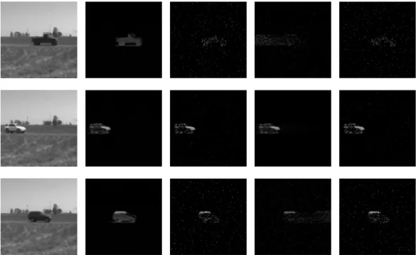
Figure 3.3: Comparison of foreground reconstruction based on 2000 measurements by the algorithms. The three rows correspond to the three sample frames. From left to right columns: the input uncompressed frame, uncompressed background subtraction, compressed background subtraction with Bayesian compressive sensing, compressed background subtrac-tion with multi-task Bayesian compressive sensing, compressed background subtracsubtrac-tion with orthogonal matching pursuit
3.3 Experiments
For the background subtraction problem the Convoy dataset (Warnell et al. 2015) is used, which consists of 260 greyscale frames and the background frame. The frames are scaled to the less resolution of 128×128to avoid memory problems. For the multitask algorithm
the batches of 40 frames are run together, while for the Bayesian compressive sensing and OMP algorithms all the frames are processed independently. There are two sets of the experiments: one withK = 2000measurements and the other withK = 5000measurements.
For both sets of the experiments all three methods are run for 10 times with 10 different design matrices Xshared among the methods. For the quantitative comparison the median values of quality measures among these runs are presented.
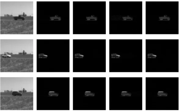
Figure 3.4: Comparison of foreground reconstruction based on 5000 measurements by the algorithms. The three rows correspond to the three sample frames. From left to right columns: the input uncompressed frame, uncompressed background subtraction, compressed background subtraction with Bayesian compressive sensing, compressed background subtrac-tion with multi-task Bayesian compressive sensing, compressed background subtracsubtrac-tion with orthogonal matching pursuit
The qualitative comparison of the models with the same design matrix X is displayed in Figures 3.3 - 3.4. The three demonstrative frames are presented. One can notice that with the same design matrix the models demonstrate similar results. The figures show that2000
measurements can be used for object region detection, while5000measurements which is
only about30%of the input resolution are enough even to distinguish parts of the objects
like doors and windows of the cars.
For the quantitative comparison of the results the following measures are used:
Reconstruction error. kβ(n)−βb (n)
k2 kβ(n)k2
,whereβ(n) is the signal ground truth, βb (n)
is the signal, reconstructed by the algorithm;
3.3 Experiments 33
Background subtraction quality measure (BS quality). |S(β(n))∩S(βb (n) )| |S(β(n))∪S(βb (n) )| , where S(β(n)) is the ground truth foreground pixels, S(βb
(n)
) is the algorithm detected
foreground pixels, | · | is the cardinality of the set;
Peak signal-to-noise ratio (PSNR). 10 log10
peakval2 MSE
,where peakval is the
maxi-mum possible pixel value, that is 255 in our case. MSE is the mean square error betweenβ(n) andβb
(n) ;
Structural similarity index (SSIM). (2µβ(n)µ
b β(n) +C1)(2σβ(n) b β(n) +C2) (µ2 β(n)+µ 2 b β(n) +C1)(σ 2 β(n)+σ 2 b β(n)+C2) , where µ β(n), µbβ (n), σ β(n), σbβ (n), σ β(n)bβ
(n) are the local means, standard deviations, and
cross-covariance for the images β(n) andβb (n)
respectively, and C1, C2 are the regularisation constants.
The difference between the uncompressed current framev(n) and the uncompressed back-ground frame b is used as the ground truth signal β(n) for every frame (the second columns
in Figures 3.3 - 3.4), since this is the signal which is compressed by (3.1).
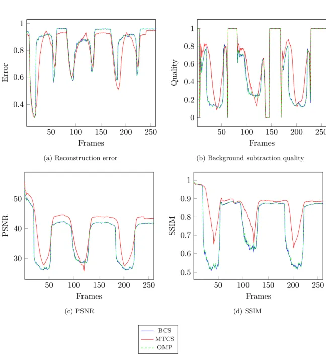
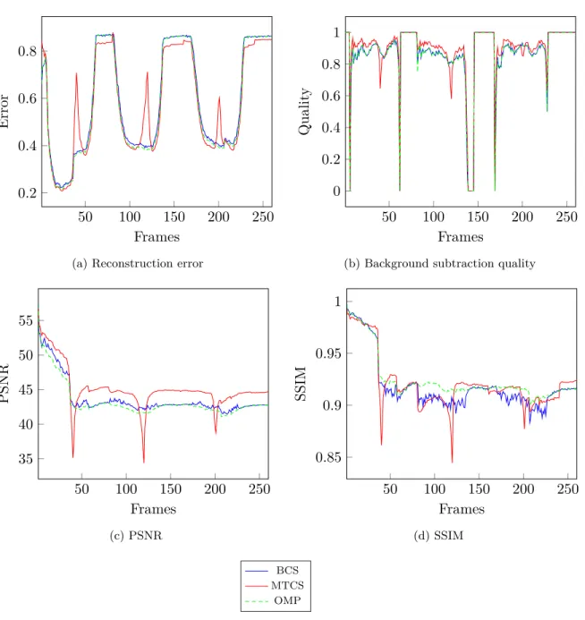
The results are presented in Figures 3.5 - 3.6. All the quality measures – reconstruction error, BS quality, PSNR and SSIM – are calculated for every frame. The mean values among the frames for each measure and computational time can be found in Tables 3.1a – 3.1b. The computational time is provided for a batch of 40 frames (BCS and OMP process each frame independently with 4 parallel workers, multitask BCS processes all 40 frames together). Implementation is made on the laptop with i7-4702HQ CPU with 2.20GHz, 16 GB RAM using MATLAB 2015a.
Multitask Bayesian compressive sensing demonstrates the best results according to almost each measure. Bayesian compressive sensing and OMP show the competitive results but Bayesian compressive sensing works faster. It is worth to note that multitask Bayesian compressive sensing has the biggest variance among the runs with the different design matrices, while the variances of the Bayesian compressive sensing and OMP runs for the same matrices are quite small.
50 100 150 200 250 0.4 0.6 0.8 1 Frames Error
(a) Reconstruction error
50 100 150 200 250 0 0.2 0.4 0.6 0.8 1 Frames Qualit y
(b) Background subtraction quality
50 100 150 200 250 30 40 50 Frames PSNR (c) PSNR 50 100 150 200 250 0.5 0.6 0.7 0.8 0.9 1 Frames SSIM (d) SSIM BCS MTCS OMP
Figure 3.5: Quantitative method comparison on the frame level for the set of the experiments with 2000 measurements
3.4 Summary
This chapter presents two Bayesian compressive sensing algorithms in the application of background subtraction. These are the applications of the Bayesian compressive sensing and of the multitask Bayesian compressive sensing algorithms. The results presented in
3.4 Summary 35 50 100 150 200 250 0.2 0.4 0.6 0.8 Frames Error
(a) Reconstruction error
50 100 150 200 250 0 0.2 0.4 0.6 0.8 1 Frames Qualit y
(b) Background subtraction quality
50 100 150 200 250 35 40 45 50 55 Frames PSNR (c) PSNR 50 100 150 200 250 0.85 0.9 0.95 1 Frames SSIM (d) SSIM BCS MTCS OMP
Figure 3.6: Quantitative method comparison on the frame level for the set of the experiments with 5000 measurements
Figures 3.3 – 3.4 demonstrate the satisfactory reconstruction quality of the original image based on only 5000 measurements (that is ≈30% of the original image size).
The conventional Bayesian compressive sensing method demonstrates the similar results to the greedy algorithm OMP but BCS is more effective in terms of the computational time.
Table 3.1: Mean quality measures
(a) Method comparison based on 2000 measurements
Algorithm Reconstruction error BS quality PSNR SSIM Time (hours)
BCS 0.8037 0.3518 34.2007 0.7198 0.23
Multitask BCS 0.7608 0.4820 37.542 0.8384 0.67
OMP 0.8028 0.3510 34.1705 0.7204 0.51
(b) Method comparison based on 5000 measurements
Algorithm Reconstruction error BS quality PSNR SSIM Time (hours)
BCS 0.4713 0.8119 43.8251 0.9186 0.9
Multitask BCS 0.4702 0.8421 45.0028 0.9212 8.5
OMP 0.4578 0.8109 43.2720 0.9266 4.8
If the computational time is not critical the extension of the Bayesian method designed for a multitask problem can improve the performance in terms of the different measures. Therefore, other extensions of the Bayesian method to include the prior information need further research.
In this chapter the components of the foreground intensities are assumed independent. For most cases the objects are grouped into several clusters, therefore more sophisticated sparsity models can be introduced to reflect the structure of the foreground. Chapter 4 presents the hierarchical sparse Bayesian model that is capable of modelling structured data.