Southern Methodist University
Southern Methodist University
SMU Scholar
SMU Scholar
Statistical Science Theses and Dissertations
Statistical Science
Fall 12-19-2020
Improved Statistical Methods for Time-series and Lifetime Data
Improved Statistical Methods for Time-series and Lifetime Data
Xiaojie Zhu
Follow this and additional works at:
https://scholar.smu.edu/hum_sci_statisticalscience_etds
Part of the
Applied Statistics Commons
,
Longitudinal Data Analysis and Time Series Commons
,
Statistical Methodology Commons
, and the
Survival Analysis Commons
Recommended Citation
Recommended Citation
Zhu, Xiaojie, "Improved Statistical Methods for Time-series and Lifetime Data" (2020). Statistical Science
Theses and Dissertations. 19.
https://scholar.smu.edu/hum_sci_statisticalscience_etds/19
This Dissertation is brought to you for free and open access by the Statistical Science at SMU Scholar. It has been
accepted for inclusion in Statistical Science Theses and Dissertations by an authorized administrator of SMU
IMPROVED STATISTICAL METHODS FOR
TIME-SERIES AND LIFETIME DATA
Approved by:
Dr. Hon Keung Tony Ng
Prof. of Statistical Science
Dr. Ian Harris
Assoc. Prof. of Statistical Science
Prof. Wayne A. Woodward
Prof. of Statistical Science
Dr. Pankaj Choudhary
IMPROVED STATISTICAL METHODS FOR
TIME-SERIES AND LIFETIME DATA
A Dissertation Presented to the Graduate Faculty of the
Dedman College
Southern Methodist University
in
Partial Fulfillment of the Requirements
for the degree of
Doctor of Philosophy
with a
Major in Statistical Science
by
Xiaojie Zhu
B. S. , Ocean Univ. of China
Ph.D., Texas A&M University
ACKNOWLEDGMENTS
This work could not have been accomplished without the wisdom of my advisor, Prof.
Ng, along with wonderful professors in the Department of Statistical Science here at SMU.
I hereby would like to thank my advisor, Professor Hon Keung Tony Ng for his constant
guidance, great encouragement and supervision. I also would like to express my sincere
gratitude to Professor Wayne Woodward for his valuable suggestions and critical insights
in this dissertation. I also would like to thank Professor Ian Harris and Professor Pankaj
Choudhary for their valuable guidance and comments. Last but not the least, my sincere
thanks are also due to my friends and colleagues and the department faculty and staff for
making my time at SMU a great experience.
I’m forever grateful to my family for being so supportive of me. I am grateful that
my husband Bo Chen is my powerful and strong pillar of strength, that my lovely kids
Maddie, Jacey and Wolfram cheer me up everyday, and that my selfless parents Benqiang
Zhu, Suhuai Lu and my caring parents-in-law Xiuying Zhou, Lejun Chen are always there
whenever I need help.
Zhu, Xiaojie
B. S. , Ocean Univ. of China
Ph.D., Texas A&M University
Improved Statistical Methods for
Time-Series and Lifetime Data
Advisor: Dr. Hon Keung Tony Ng
Doctor of Philosophy degree conferred December 19, 2020
Dissertation completed July 9, 2020
In this dissertation, improved statistical methods for time-series and lifetime data are
developed. First, an improved trend test for time series data is presented. Then, robust
parametric estimation methods based on system lifetime data with known system
signa-tures are developed.
In the first part of this disseration, we consider a test for the monotonic trend in time
series data proposed by Brillinger (1989). It has been shown that when there are highly
correlated residuals or short record lengths, Brillinger’s test procedure tends to have
sig-nificance level much higher than the nominal level. This could be related to the
discrep-ancy between the empirical distribution of the test statistic and the asymptotic normal
distribution. Hence, different bootstrap-based procedures are proposed based on the
Brillinger test statistic. The performances of proposed bootstrap test procedures are
eval-uated through an extensive Monte Carlo simulation study, and are compared to other
trend test procedures in the literature.
In the second part of this dissertation, we consider the estimation of component
re-liability based on system lifetime data with known system signature using the minimum
density divergence estimation method. Different estimation procedures based on the
min-imum density divergence estimation method are proposed. We also study the standard
error estimation and interval estimation procedures for the proposed minimum density
di-vergence estimator. Based on the proposed procedures, a Monte Carlo simulation study
is used to evaluate the performance of these proposed procedures and compare these
procedures with the maximum likelihood estimation under different contaminated
mod-els. Then, a numerical example is presented to illustrate the minimum density divergence
estimation method. In particular, we show that the proposed estimation procedures are
robust to contamination and model misspecification.
TABLE OF CONTENTS
LIST OF FIGURES . . . .
viii
LIST OF TABLES . . . .
xii
CHAPTER
1.
Introduction . . . .
1
1.1. Introduction of Improved Test for Monotonic Trend in Time Series Data . . .
2
1.2. Introduction of Robust Parameter Estimation Based on System
time
Data
.
.
.
.
.
.
.
.
.
.
.
.
.
.
.
.
.
.
.
.
.
.
.
.
.
.
.
.
.
.
.
.
.
.
.
.
.
.
.
.
.
.
.
.
.
.
.
.
.
.
.
.
.
.
.
.
.
.
.
.
.
4
1.3. Scope of The Dissertation. . . .
6
2.
Improved Test for Monotonic Trend in Time Series Based on Resampling
Method
.
.
.
.
.
.
.
.
.
.
.
.
.
.
.
.
.
.
.
.
.
.
.
.
.
.
.
.
.
.
.
.
.
.
.
.
.
.
.
.
.
.
.
.
.
.
.
.
.
.
.
.
.
.
.
.
.
.
.
.
.
.
.
.
.
.
.
.
8
2.1. The Issue of Inflated Significance Levels . . . .
8
2.2. Test Procedures Based on Bootstrap Methods . . . .
12
2.3. Performance of the Proposed Procedures . . . .
15
2.3.1. Significance Level . . . .
16
2.3.2. Power . . . .
20
2.4. Comparison with Other Trend Tests . . . .
22
2.5. Illustrative Example . . . .
25
3.
Robust Parameter Estimation of Component Lifetime Distribution based on
System
Lifetime
with
Known
Signature
.
.
.
.
.
.
.
.
.
.
.
.
.
.
.
.
.
.
.
.
.
.
.
.
.
.
.
.
.
.
.
.
.
.
.
.
.
27
3.1. System Lifetime Data . . . .
27
3.2. Minimum Density Divergence Estimator for System Lifetime Data . . . .
29
3.2.1. Minimum Density Divergence Estimator . . . .
29
3.2.2. Standard Error Estimation and Confidence Intervals . . . .
33
3.2.2.2. Based on The Observed Fisher Information Matrix . . . .
36
3.2.2.3. Based on The Bootstrap Method . . . .
37
3.3. Monte Carlo Simulation Studies . . . .
38
3.3.1. Results for Estimation of Scale and Shape Parameters . . . .
39
3.3.1.1. Results for The
M DE
S
Procedure . . . .
39
3.3.1.2. Results for The
M DE
C
Procedure . . . .
49
3.3.1.3. Results for The
M DE
P
Procedure . . . .
52
3.3.2. Results for Estimating The Mean Component Lifetime . . . .
71
3.3.3. Results for Standard Error Estimation and Confidence Interval
Estimation
.
.
.
.
.
.
.
.
.
.
.
.
.
.
.
.
.
.
.
.
.
.
.
.
.
.
.
.
.
.
.
.
.
.
.
.
.
.
.
.
.
.
.
.
.
.
.
.
.
.
.
.
.
75
3.3.3.1. Determining a Suitable Bootstrap Size for Standard
Error
Estimation
.
.
.
.
.
.
.
.
.
.
.
.
.
.
.
.
.
.
.
.
.
.
.
.
.
.
.
.
.
.
.
.
.
.
.
.
.
.
78
3.3.3.2. Performance of Standard Error Estimates . . . .
79
3.3.3.3. Performance of Confidence Intervals . . . .
79
3.4. Illustrative Example . . . .
83
4.
Concluding Remarks and Future Research Directions . . . .
93
4.1. Concluding Remarks . . . .
93
4.1.1. Improved Test for Monotonic Trend in Time Series Data . . . .
93
4.1.2. Robust Parameter Estimation for System Lifetime Data . . . .
94
4.2. Future Research Directions . . . .
95
4.2.1. Improved Test for Monotonic Trend in Time Series Data . . . .
95
LIST OF FIGURES
Figure
Page
2.1
The empirical distributions of Brillinger’s test statistic (blue solid curves)
and the standard normal distributions (red solid curves) with different
record lengths. (a)
T
= 100
, (b)
T
= 500
, (c)
T
= 1000
and (d)
T
= 10000
. The black dash lines demonstrate the observed test
statistic, the blue dash lines are the critical values for rejecting the
null hypothesis based on the empirical distributions, the red dash
lines are the critical value for rejecting the null hypothesis based on
the asymptotic standard normal.. . . .
11
2.2
The variance of estimated significance and observed power for
Proce-dure 1, ProceProce-dure 2, and ProceProce-dure 3 with different record lengths.
The blue circle lines are for
T
= 100
, the red star lines are for
T
= 500
,
and the purple cross lines are for
T
= 1000
.
. . . .
17
2.3
Estimated significance levels of the three proposed bootstrap-based
pro-cedures (black for Procedure 1, blue for Procedure 2 and red for
Pro-cedure 3) with parametric and nonparametric bootstrap methods,
dif-ferent record lengths and autocorrelation coefficients. The dots
rep-resent the values of the estimated significance levels and the error
bars represent the Monte Carlo error.
. . . .
19
2.4
(a) Estimated power of the three proposed bootstrap-based procedures
(black for Procedure 1, blue for Procedure 2 and red for Procedure 3)
for
S
(
t
) =
√
t
and signal-to-noise ratio of 1, with parametric (dots) and
nonparametric (triangles)bootstrap methods. (b) Estimated power
values of the three proposed bootstrap-based procedures (black for
Procedure 1, blue for Procedure 2 and red for Procedure 3) for
S
(
t
) =
√
t
and parametric bootstrap method, with signal-to-noise ratios(S/N)
of 0.25 (dots) and 4.0 (triangles). The dots and triangles represent
the values of estimated power and the error bars represent the Monte
Carlo error.
. . . .
21
2.5
Global annual temperature anomaly (black solid line) from 1880 to 2016
with fifteen years running mean of annual data (blue dash line)
. . . .
26
3.1
(a) a 4-component series-parallel III system (
s
= (1
/
4
,
1
/
4
,
1
/
2
,
0)
,
re-ferred to as
system I) and (b) a 4-component mixed parallel I system
3.2
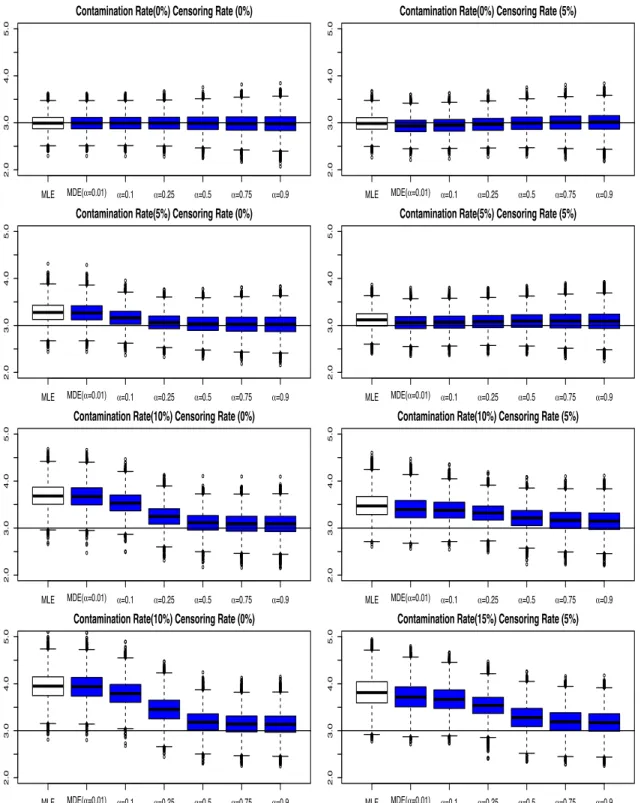
Boxplot of 10000 estimates of scale parameters by the
M DE
S
procedure
for the System I with the longer-life contamination model
. . . .
40
3.3
Boxplot of 10000 estimates of scale parameters by the
M DE
S
procedure
for the System I with the shorter-life contamination model
. . . .
41
3.4
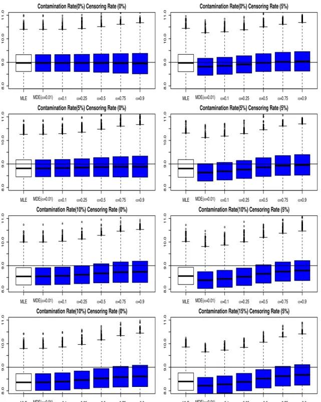
Boxplot of 10000 estimates of shape parameters by the
M DE
S
proce-dure for the System I with the longer-life contamination model
. . . .
42
3.5
Boxplot of 10000 estimates of shape parameters by the
M DE
S
proce-dure for the System I with the shorter-life contamination model
. . . .
43
3.6
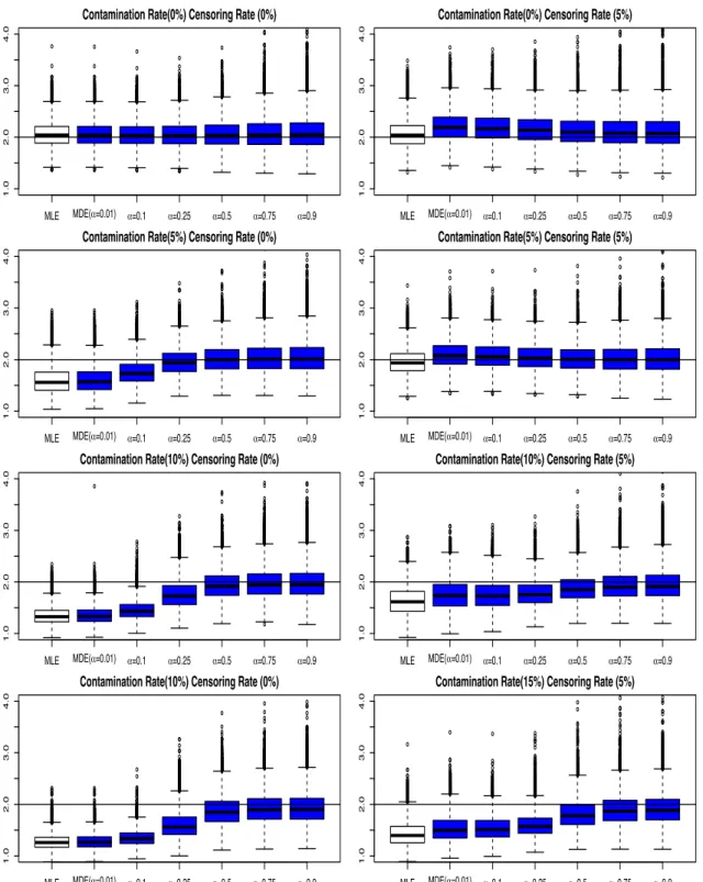
Boxplot of 10000 estimates of scale parameters by the
M DE
S
procedure
for the System II with the longer-life contamination model
. . . .
44
3.7
Boxplot of 10000 estimates of scale parameters by the
M DE
S
procedure
for the System II with the shorter-life contamination model
. . . .
45
3.8
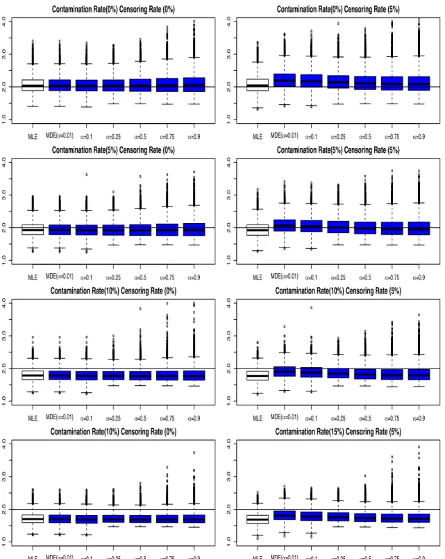
Boxplot of 10000 estimates of shape parameters by the
M DE
S
proce-dure for the System II with the longer-life contamination model
. . . .
46
3.9
Boxplot of 10000 estimates of shape parameters by the
M DE
S
proce-dure for the System II with the shorter-life contamination model
. . . .
47
3.10
Relative efficiencies of estimated scale parameter by the
M DE
S
proce-dure for the System I
. . . .
50
3.11
Relative efficiencies of estimated shape parameter by the
M DE
S
proce-dure for the System I
. . . .
50
3.12
Relative efficiencies of estimated scale parameter by the
M DE
S
proce-dure for the System II
. . . .
51
3.13
Relative efficiencies of estimated shape parameter by the
M DE
S
proce-dure for the System II
. . . .
51
3.14
Boxplot of 10000 estimates of scale parameters by the
M DE
C
procedure
for the System I with the longer-life contamination model
. . . .
53
3.15
Boxplot of 10000 estimates of scale parameters by the
M DE
C
procedure
for the System I with the shorter-life contamination model
. . . .
54
3.16
Boxplot of 10000 estimates of shape parameters by the
M DE
C
proce-dure for the System I with the longer-life contamination model
. . . .
55
3.17
Boxplot of 10000 estimates of shape parameters by the
M DE
C
3.18
Boxplot of 10000 estimates of scale parameters by the
M DE
C
procedure
for the System II with the longer-life contamination model
. . . .
57
3.19
Boxplot of 10000 estimates of scale parameters by the
M DE
C
procedure
for the System II with the shorter-life contamination model
. . . .
58
3.20
Boxplot of 10000 estimates of shape parameters by the
M DE
C
proce-dure for the System II with the longer-life contamination model
. . . .
59
3.21
Boxplot of 10000 estimates of shape parameters by the
M DE
C
proce-dure for the System II with the shorter-life contamination model
. . . .
60
3.22
Relative efficiencies of estimated scale parameter by the
M DE
C
proce-dure for the System I
. . . .
61
3.23
Relative efficiencies of estimated shape parameter by the
M DE
C
proce-dure for the System I
. . . .
61
3.24
Relative efficiencies of estimated scale parameter by the
M DE
C
proce-dure for the System II
. . . .
62
3.25
Relative efficiencies of estimated shape parameter by the
M DE
C
proce-dure for the System II
. . . .
62
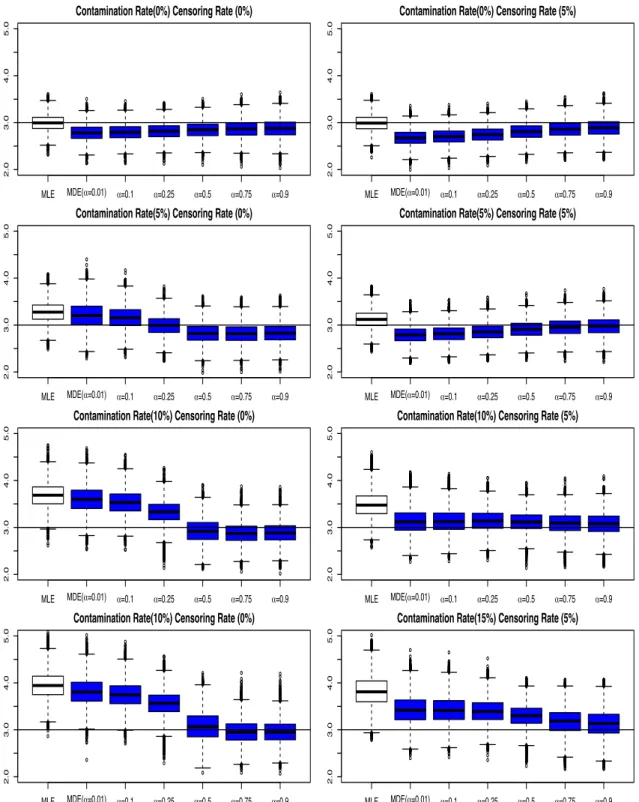
3.26
Boxplot of 10000 estimates of scale parameters by the
M DE
P
procedure
for the System I with the longer-life contamination model
. . . .
63
3.27
Boxplot of 10000 estimates of scale parameters by the
M DE
P
procedure
for the System I with the shorter-life contamination model
. . . .
64
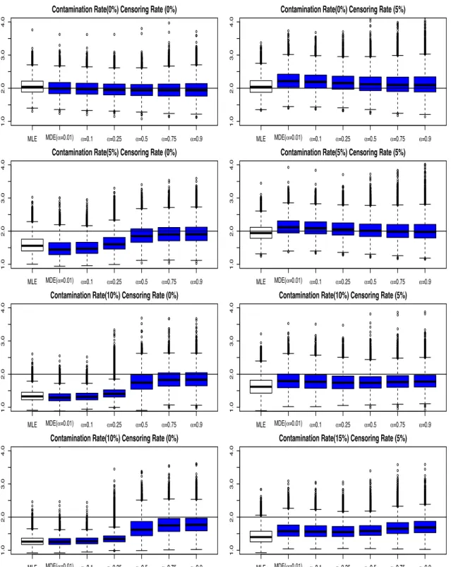
3.28
Boxplot of 10000 estimates of shape parameters by the
M DE
P
proce-dure for the System I with the longer-life contamination model
. . . .
65
3.29
Boxplot of 10000 estimates of shape parameters by the
M DE
P
proce-dure for the System I with the shorter-life contamination model
. . . .
66
3.30
Boxplot of 10000 estimates of scale parameters by the
M DE
P
procedure
for the System II with the longer-life contamination model
. . . .
67
3.31
Boxplot of 10000 estimates of scale parameters by the
M DE
P
procedure
for the System II with the shorter-life contamination model
. . . .
68
3.32
Boxplot of 10000 estimates of shape parameters by the
M DE
P
proce-dure for the System II with the longer-life contamination model
. . . .
69
3.33
Boxplot of 10000 estimates of shape parameters by the
M DE
P
3.34
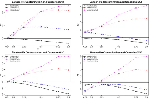
Relative efficiencies of estimated scale parameter by the
M DE
P
proce-dure for the System I
. . . .
72
3.35
Relative efficiencies of estimated shape parameter by the
M DE
P
proce-dure for the System I
. . . .
72
3.36
Relative efficiencies of estimated scale parameter by the
M DE
P
proce-dure for the System II
. . . .
73
3.37
Relative efficiencies of estimated shape parameter by the
M DE
P
proce-dure for the System II
. . . .
73
3.38
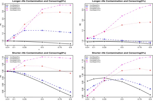
Relative efficiencies of estimated mean component lifetime for the
Sys-tem I with the longer-life contamination model
. . . .
76
3.39
Relative efficiencies of estimated mean component lifetime for the
Sys-tem I with the shorter-life contamination model
. . . .
76
3.40
Relative efficiencies of estimated mean component lifetime for the
Sys-tem II with the longer-life contamination model
. . . .
77
3.41
Relative efficiencies of estimated mean component lifetime for the system
II with the shorter-life contamination model
. . . .
77
3.42
Coefficient of variation of
SE
c
B
for scale parameter as a function of the
number of bootstrap samples
B . . . .
80
3.43
Coefficient of variation of
SE
c
B
for scale parameter as a function of the
number of bootstrap samples
B . . . .
80
4.1
Percentage of identifying a significant trend for testing the monotonic
trend with (a) the smooth window for spectrum
L
= 7
and the moving
average parameter
V
varying from 2 to 20 in interval of 2 and with
(b) the moving average parameter
V
= 5
and the smooth window for
LIST OF TABLES
Table
Page
2.1
Estimated significance levels (in %) of the Brillinger test for 1000
replica-tions of the model in Eq. (
1.1
) with a constant
S
(
t
)
and
E
(
t
)
in form
of
(1
−
φ
1
B
)
E
(
t
) =
a
(
t
)
, where
a
(
t
)
is a
N
(0
,
1)
Gaussian white noise
. . . .
9
2.2
Brillinger’s test statistic, average of
q
2
π
f
ˆ
EE
(0)
P
T
t
=1
[
c
(
t
)]
2
and standard
error of
L
=
P
T
t
=1
c
(
t
)
Y
(
t
)
for the 500 simulated time series sample of
the model
Y
(
t
)
with a constant signal term
S
(
t
)
and an AR(1) residual
(1
−
0
.
95
B
)
E
(
t
) =
a
(
t
)
, where
a
(
t
)
is a
N
(0
,
1)
white noise series.
. . . .
13
2.3
Estimated power (in %) for the three proposed bootstrap-based
proce-dures (parametric bootstrap) for different record lengths and different
forms of trends.
. . . .
22
2.4
Estimated significance level (in %) for simulations.
. . . .
25
3.1
The 24 possible arrangements of the component lifetime in a 4-component
series-parallel III system
. . . .
30
3.2
Simulated standard errors the
M DE
S
and the averaged standard error
estimates based on the theoretical results from
Basu et al.
(
1998
)
(
SE
c
A
), based on observed Fisher information matrix (
SE
c
F
), and based
on bootstrap method (
SE
c
B
) with bootstrap size
B
= 250
. . . .
81
3.3
Simulated coverage probabilities (in %) and average widths of confidence
intervals of the scale parameter computed based on MLE and
M DE
S
with different values of
α
under the longer-life and shorter-life
contam-ination models for System I
. . . .
84
3.4
Simulated coverage probabilities and average widths of confidence
inter-vals of the shape parameter computed based on MLE and
M DE
S
with different values of
α
under the longer-life and shorter-life
con-tamination models for System I
. . . .
85
3.5
Simulated coverage probabilities and average widths of confidence
in-tervals of the scale parameter computed based on MLE and
M DE
S
with different values of
α
under the longer-life and shorter-life
3.6
Simulated coverage probabilities and average widths of confidence
inter-vals of the shape parameter computed based on MLE and
M DE
S
with different values of
α
under the longer-life and shorter-life
con-tamination models for System II
. . . .
87
3.7
Simulated system lifetimes with system signature
s
= (1
/
4
,
1
/
4
,
1
/
2
,
0)
with component lifetime distribution
W eibull
(3
,
2)
. . . .
88
3.8
Simulated system lifetimes with system signature
s
= (1
/
4
,
1
/
4
,
1
/
2
,
0)
with component lifetime distribution of
W eibull
(3
,
2)
and one
contam-inated observation from
W eibull
(9
,
2)
. . . .
88
3.9
Point and interval estimates for Weibull scale parameter for the data set
presented in Table
3.7
. . . .
90
3.10
Point and interval estimates for Weibull shape parameter for the data set
presented in Table
3.7
. . . .
91
3.11
Point and interval estimates for Weibull scale parameter for the data set
presented in Table
3.8
. . . .
92
3.12
Point and interval estimates for Weibull shape parameter for the data set
Chapter 1
Introduction
The time dimension is an essential part in academic research. There are tremendous
observations along the time domain in many fields of studies, such as economics,
clima-tology, physics, chemistry, medical science and social sciences etc. When we analyze
measurements at each time points along a time line, we are dealing with time series data.
On the other hand, when we consider the time from an origin to an event that occurs, we
are dealing with time-to-event (lifetime/reliability/survival) data. We accordingly study the
two fields related to time - time series analysis and time-to-event data analysis - in this
dissertation.
In the analysis of time series data, one of the fundamental questions of interest is
whether there is a trend in the time series. The study of trends in times series is important
in many applications, such as in the scientific study of climate (
Cohn and Lins
,
2005
;
Woodward and Gray
,
1993
), in temperature and precipitation (
Feidas et al.
,
2004
;
Xu
et al.
,
2002
), in meteorology (
Bonaccorso et al.
,
2005
), and in economics. Detecting
trends in a time series has been discussed in the literature for linear trends (
Bloomfield
and Nychka
,
1992
;
Cochrane and Orcutt
,
1949
;
Sun and Pantula
,
1999
;
Woodward and
Gray
,
1993
,
1995
;
Woodward et al.
,
1997
), for quadratic trends (
Woodward and Gray
,
1995
;
Woodward
,
2003
) and for monotonic trends (
Balakrishnan et al.
,
2016
;
Brillinger
,
1989
;
Hofmann and Balakrishnan
,
2006
). For example, for temperature data, if there is
indeed an underlying trend in the data, it is typically either linear or quadratic. In the first
part of this dissertation, we focus on the general case of detecting monotonic trends.
In the second part, statistical analysis of system lifetime data with known system
struc-ture is considered. System lifetime data are commonly encountered in industrial or
en-gineering settings where
n
components form a system and only the failure time of the
system can be observed. Methods for estimating parameters of component lifetime
dis-tributions based on observed system lifetime data have been discussed in the literature
(
Balakrishnan et al.
,
2011a
;
Balakrishnan et al.
,
2011b
;
Ng et al.
,
2012
;
Yang et al.
,
2016
;
Zhang et al.
,
2015
). However, these classical estimation methods may perform poorly in
estimating component reliability when there are contaminations and/or outliers in the
ob-served system lifetime data. To resolve this, we propose a robust parametric estimation
for component lifetime distribution using the minimum density divergence method (
Basu
et al.
,
1998
) based on system lifetime data.
1.1. Introduction of Improved Test for Monotonic Trend in Time Series Data
In the study of tests for monotonic trends, we consider a general form of trend in which
the time series
Y
(
t
)
,
t
= 1
,
2
, . . . , T
, is decomposed as
Y
(
t
) =
S
(
t
) +
E
(
t
)
,
(1.1)
where
S
(
t
)
is a signal series and
E
(
t
)
is a stationary zero-mean noise series. The noise
series
E
(
t
)
could be a stationary white noise process, or a stationary zero-mean
autore-gressive process. The hypothesis of interest is whether
S
(
t
)
has no trend or a monotonic
trend.
To test the hypothesis that
S
(
t
)
has no trend or a monotonic trend, Brillinger (
Brillinger
,
L
=
T
X
t
=1
c
(
t
)
Y
(
t
)
,
(1.2)
where the coefficient
c
(
t
)
is defined as
c
(
t
) =
t
1
−
t
T
1
/
2
−
(
t
+ 1)
1
−
t
+ 1
T
1
/
2
.
If the noise series
E
(
t
)
is independent and identically distributed (i.i.d.) white noise, i.e.,
N
(0
, σ
2
)
, then the mean and variance of
L
are respectively
P
T
t
=1
c
(
t
)
S
(
t
)
and
σ
[
P
T
t
=1
c
(
t
)]
2
,
and we can use the test statistic in the form of
P
T
t
=1
c
(
t
)
S
(
t
)
/σ
[
P
T
t
=1
c
(
t
)]
2
. However,
when the noise series is a zero-mean autocorrelated process, while the mean of
L
is
still
P
T
t
=1
c
(
t
)
S
(
t
)
, the variance of
L
is no longer
σ
[
P
T
t
=1
c
(
t
)]
2
. Brillinger (
Brillinger
,
1989
)
assumed that the cumulant function of the noise series
E
(
t
)
is finite and the signal series
S
(
t
)
is square integrable and has finite Lipshitz integral modulus of continuity. Under these
assumptions, the variance of
L
can be obtained as
2
πf
EE
(0)
P
T
t
=1
[
c
(
t
)]
2
, with
f
EE
(0)
being
the power spectrum of the noise series
E
(
t
)
at frequency of 0. In our study, we consider
time series with an autocorrelated noise series
E
(
t
)
satisfying
φ
(
B
)
E
(
t
) =
a
(
t
)
, where
φ
(
B
) = 1
−
φ
1
B
− · · · −
φ
p
B
p
,
B
is the back-shift operator such that
B
k
E
(
t
) =
E
(
t
−
k
)
, and
a
(
t
)
,
t
= 1
,
2
, . . . , T
are i.i.d. normally distributed, denoted as
a
(
t
)
∼
N
(0
, σ
2
a
)
. For a large
T
(i.e., a long record length), the distribution of
L
is proved to be asymptotically normal
(
Brillinger
,
1989
).
Under the null hypothesis of a constant signal
S
(
t
)
, the distribution of
L
becomes
asymptotically normal with mean 0 and variance
2
πf
EE
(0)
P
T
t
=1
[
c
(
t
)]
2
. The test statistic
proposed by Brillinger (
Brillinger
,
1989
),
T
1
=
P
T
t
=1
c
(
t
)
Y
(
t
)
{
2
πf
EE
(0)
P
T
t
=1
[
c
(
t
)]
2
}
1
2
,
(1.3)
is asymptotically distributed as standard normal. We refer to the test statistics
T
1
in Eq.
(
1.3
) as Brillinger’s test statistic hereafter. In practice,
2
π
f
ˆ
EE
(0)
P
T
t
=1
[
c
(
t
)]
2
is used to
estimate the variance of
L, where
f
ˆ
EE
(0)
is a smoothed periodogram spectral estimate.
When testing a linear trend in time series, several testing procedures, such as the
Cochran-Orcutt (CO) procedure (
Cochrane and Orcutt
,
1949
), the maximum likelihood
procedure, and the Bloomfield and Nychka (BN) procedure (
Bloomfield and Nychka
,
1992
), tend to have a significance level higher than the nominal level when the time
se-ries is strongly auto-correlated and/or with short to moderate record lengths (
Park and
Michell
,
1980
;
Woodward and Gray
,
1993
;
Woodward et al.
,
1997
). To solve the
inflated-significance problem,
Woodward et al.
(
1997
) proposed an improved test for linear trends
using the empirical distribution of the test statistic of the CO procedure from bootstrap
samples.
In our study, it is found that the Brillinger test statistic also has the inflated-significance
problem when the time series is strongly auto-correlated. We will provide further detailed
discussions of this inflated-significance problem in Chapter 2. In the sequel, we propose
improved tests for monotonic trends using the Brillinger test statistic, by adopting the
bootstrap idea from
Woodward et al.
(
1997
).
1.2. Introduction of Robust Parameter Estimation Based on System Lifetime Data
We first formally describe a system with
n
components, where only the failure time of
the system can be observed. Suppose the
n
component’ lifetimes,
X
1
, X
2
, ..., X
n
, are i.i.d.
with probability density function (p.d.f.)
f
X
(
t
;
θ
)
, cumulative distribution function (c.d.f.)
F
X
(
t
;
θ
)
, and survival function (s.f.)
F
¯
X
(
t
;
θ
)
. The ordered component lifetimes are
X
1:
n
<
X
2:
n
... < X
n
:
n
, where
X
i
:
n
is the
i-th ordered component lifetime. The failure of the whole
system, measured by the system lifetime
T
, depends on the order of failure time of the
n
components. Accordingly, we define a system signature as an
n-element probability
vector
s
= (
s
1
, s
2
, ..., s
n
)
, where
s
i
is the probability that the
i-th ordered component failure
Note that the system signature depends on the system structrue only, and is distribution
free. With a known system signature, the p.d.f. and s.f. of the system lifetime
T
for an
n-component system can be expressed respectively as (
Kochar et al.
,
1999
):
f
T
(
t
;
θ
) =
n
X
i
=1
s
i
n
i
if
X
(
t
;
θ
) [
F
X
(
t
;
θ
)]
i
−
1
¯
F
X
(
t
;
θ
)
n
−
i
,
(1.4)
and
¯
F
T
(
t
;
θ
) =
n
X
i
=1
s
i
i
−
1
X
j
=0
[
F
X
(
t
;
θ
)]
j
¯
F
X
(
t
;
θ
)
n
−
j
.
(1.5)
Based on the p.d.f. and s.f. of the system lifetime
T
, statistical inference of the
com-ponent lifetime distribution based on system lifetime data with a known system signature
has been discussed extensively in the literature. For example,
Balakrishnan et al.
(
2011a
)
developed an exact nonparametric inference for population quantiles and tolerance limits
of the component lifetime distribution in a system.
Balakrishnan et al.
(
2011b
) derived
the best linear unbiased estimator (BLUE) for the component lifetime of reliability systems
with known signatures.
Ng et al.
(
2012
) discussed the method of moments, the maximum
likelihood method and the least squares method for system lifetime data based on a
pro-portional hazard rate model.
Chahkandi et al.
(
2014
) proposed nonparametric methods to
construct prediction intervals for the lifetime of a system with known signature.
Zhang et
al.
(
2015
) proposed a regression-based method for model parameters of the component
lifetime in a censored system failure data with known signature.
Yang et al.
(
2016
)
pro-posed a stochastic expectation-maximization (SEM) algorithm for obtaining the maximum
likelihood estimates of the parameters in component lifetime distribution based on system
lifetimes. More recently,
Yang et al.
(
2019
) developed the expectation maximization
algo-rithm to obtain the maximum likelihood estimates (MLEs) of the parameters in component
lifetime distribution based on system lifetime data when the system structure is unknown.
In industrial experiments on systems, there are many situations in which the
under-lying system is removed from experimentation before the occurrence of a failure of the
system. Two common reasons for such pre-planned censoring are saving the time on
test and reducing the cost associated with the experiment because failure implies the
de-struction of a system, which can be costly (
Cohen
,
1991
;
Meeker and Escobar
,
1998
).
In this dissertation, we consider a Type-II right censoring scheme in which the number
of observed failures is pre-specified as
r
and the experiment is terminated as soon as a
r-th ordered system failure is observed. Several studies on the Type-II censored system
lifetime data with system signature have been conducted (
Balakrishnan et al.
,
2011b
;
Ng
et al.
,
2012
;
Yang et al.
,
2016
,
2019
;
Zhang et al.
,
2015
).
Finally, when there are contaminations or outliers in observed lifetime data, the
perfor-mance of the maximum likelihood or other classical estimation methods may be affected,
resulting in poor estimates of the component reliability characteristics.
Basu et al.
(
1998
)
developed a family of density-based divergences measure with a single power parameter
α
that controls the trade-off between robustness and efficiency, and proposed a procedure
for estimating model parameters based on minimizing the density divergence.
Base et al.
(
2006
) further extended the minimum density divergence procedure to censored survival
data with and without contamination, and found that the minimum density divergence
es-timator (M DE) is superior than the MLE when there is contamination in the censored
survival data.
In our study, we propose to use the MDE for parameter estimation of component
re-liability based on system lifetime data with and without contamination. For lifetime data,
since censoring is a common feature as a result of time or budget constraints, we consider
Type-II censoring in this study (
Cohen
,
1991
;
Meeker and Escobar
,
1998
), and evaluate
the performance of the
M DE
with and without the Type-II censoring.
1.3. Scope of The Dissertation
In Chapter 2, we investigate the-inflated-significance-level problem in the Brillinger test
for testing monotonic trends. As mentioned, the Brillinger test can have an inflated
sig-nificance level, especially when the autoregressive process is strong in time series. This
could be caused by the differences between the empirical distribution of the Brillinger
test statistic and the asymptotic normal distribution of the Brillinger test statistic. We
pro-pose three different bootstrap testing procedures for testing monotonic trends, based on
the Brillinger test statistic. In order to evaluate the performance of the three proposed
bootstrap-based procedures, we then carry out a Monte Carlo simulation study under
different settings. The observed significance level and the power of proposed
bootstrap-based procedures are further investigated and compared with the Brillinger test
proce-dure. Moreover, the proposed bootstrap-based procedures are also compared with four
other trend testing procedures in the literature.
In Chapter 3, we discuss robust parameter estimation of the component lifetime
dis-tribution based on system lifetime data. In the literature, parametric and nonparametric
estimation of the component lifetime distribution based on system lifetime data have been
developed. However, some methods have poor performance when there are
contam-inations in the data. To resolve this issue, we adopt the minimum density divergence
estimator to system lifetime data to make statistical inference of component lifetime
distri-bution, and propose three procedures based on the minimum density divergence
estima-tor. In addition, we conduct a Monte Carlo simulation to evaluate the performance of the
proposed minimum density divergence estimation procedures, and provide an illustrative
example to illustrate the proposed estimation methods for component lifetime distribution
based on system lifetime data.
Finally, in Chapter 4, we present some concluding remarks with some
recommenda-tions on the two studies, testing for monotonic trends and robust parameter estimation of
component lifetime based on system lifetime data. We also provide some possible future
research directions based on these two studies.
Chapter 2
Improved Test for Monotonic Trend in Time Series Based on Resampling Method
In this chapter, we present the improved monotonic trend test based on the Brillinger
test statistic. In Section 2.1, we illustrate the issue of inflated significance level of the
Brillinger test and analyze the possible reasons for this issue. By adopting the resampling
method, three different bootstrap testing procedures based on Brillinger’s test statistic
are proposed in Section 2.2. In Section 2.3, a Monte Carlo simulation study is used to
evaluate the performance of the proposed bootstrap-based procedures in terms of their
significance levels and power values under different settings. In Section 2.4, the
pro-posed procedures are compared with four other trend testing procedures and are further
discussed on their performance under different scenarios. In Section 2.5, the proposed
methodologies are illustrated by testing for trend in the annual global mean temperature
anomaly from 1880 to 2016.
2.1. The Issue of Inflated Significance Levels
When there are highly correlated residuals or short record lengths, Brillinger’s test
procedure tends to have a significance level much higher than the nominal level. To
illustrate this inflated-significance issue in the Brillinger test procedure, we first conduct a
preliminary Monte Carlo simulation study. In the simulation study, we generate time series
based on the model in Eq. (
1.1
), assuming a constant
S
(
t
)
and a noise series
E
(
t
)
with
a first-order autoregressive (AR(1)) structure (i.e.,
φ
(
B
) = 1
−
φ
1
B). We consider eight
autoregressive coefficients
φ
1
= 0
.
8
and
0
.
95
. For each setting, 1000 replications are used
to estimate the significance level of the Brillinger test.
The estimated significance levels of the Brillinger test under different settings are
pre-sented in Table
2.1
. We can see that with an autoregressive coefficient of 0.95, the
es-timated significance level for testing monotonic trends is 76% for a record length of 100,
and reaches 4.9% only when the record length becomes 25000. With a smaller
autore-gressive coefficient (φ
1
= 0
.
8
), the inflated-significance problem is less severe; however,
the estimated significance levels are still higher than 8% for record lengths
T
= 100
, 500
and 1000, indicating the existence of an inflated-significance problem in the Brillinger test
procedure when the autocorrelation is strong and/or when the record length is short. In
the sequel of this section, we refer to small sample size as
T
≤
200
, moderate sample
size as
200
< T
≤
1000
, and large sample size as
T >
1000
for convenience.
One plausible reason for the inflated-significance-level problem is that the actual
small-sample sampling distribution of the test statistic cannot be well approximated by a normal
distribution. In order to study the sampling distribution of Brillinger’s test statistic, we
simulate time series from the model in Eq. (
1.1
) with a constant signal series
S
(
t
)
and
an AR(1) residual series,
(1
−
φ
1
B
)
E
(
t
) =
a
(
t
)
, where
a
(
t
)
is an i.i.d.
N
(0
,
1)
Gaussian
white noise series. Fixing the autocorrelation coefficient
φ
1
to be 0.95, we set the record
length
T
to be 100, 500, 1000 and 10000. For each simulated time series with a certain
record length, we estimate the autoregressive coefficients
φ
1
, denoted as
φ
ˆ
1
, for the noise
series by assuming a constant signal term
S
(
t
)
. With the estimated coefficient
φ
ˆ
1
, we
Table 2.1: Estimated significance levels (in %) of the Brillinger test for 1000 replications
of the model in Eq. (
1.1
) with a constant
S
(
t
)
and
E
(
t
)
in form of
(1
−
φ
1
B
)
E
(
t
) =
a
(
t
)
,
where
a
(
t
)
is a
N
(0
,
1)
Gaussian white noise
Record length (T
)
100
500
1000
5000
10000
15000
20000
25000
φ
1
= 0
.
95
76.0
50.0
32.6
14.0
8.9
7.9
5.9
4.9
then generate 500 bootstrap samples (N
b
= 500
) from the associated AR(1) time series
and calculate Brillinger’s test statistic for each bootstrap sample. To illustrate the
obser-vations from the simulation study, the histograms and the estimated density curves (blue
curves) for Brillinger’s test statistics of the 500 simulated samples are compared with the
asymptotic normal distribution (red curves) in Figure
2.1
for one of the simulations.
Figure
2.1
demonstrates that there are substantial discrepancies between the
em-pirical distribution of Brillinger’s test statistic,
T
1
, and the standard normal distribution,
especially for short record length and large autoregressive coefficient
φ
1
. For example,
with a record length of 100, both empirical distribution and standard normal distribution
are centered at 0, but the empirical distribution of
T
1
has a much fatter tail compared to
the standard normal distribution (Figure
2.1
a). As a result, the absolute values of the
crit-ical values for rejecting the null hypothesis based on the empircrit-ical distribution of
T
1
(blue
dashed lines in Figure
2.1
a) are larger than those critical values based on the standard
normal distribution (red dashed lines in Figure
2.1
a). Hence, for example, with the value
of the test statistic
T
1
being 14.78 (black dashed line in Figure
2.1
a), we fail to reject the
null hypothesis based on the empirical distribution of
T
1
, but reject the null hypothesis
based on the standard normal distribution.
We also observe that when the record length increases, the discrepancies between
the empirical distribution of
T
1
and the standard normal distribution become smaller, as
is to be expected. When the record length increases to 500 and 1000, the empirical
distributions of Brillinger’s test statistics become closer to the standard normal distribution,
but they still have relatively heavier tails compared to the standard normal distribution
(Figures
2.1
b and
2.1
c). When the record length reaches 10000, the empirical distribution
of Brillinger’s test statistic shows a bell shape similar to the standard normal distribution
(Figure
2.1
d). These observations suggest that the asymptotic normal approximation
works well for long record lengths, which verifies the results in
Brillinger
(
1989
).
In order to further investigate the reason for inflated significance level, we study the
accuracy of the variance estimate of the linear combination
L
in Eq. (
1.2
) using Monte
T=100
Density
−30
−20
−10
0
10
20
30
0.0
0.1
0.2
0.3
0.4
0.5
emperical distribution of
T
1
Standard Normal
T=500
Density
−10
−5
0
5
10
0.0
0.1
0.2
0.3
0.4
0.5
T=1000
Density
−6
−4
−2
0
2
4
6
0.0
0.1
0.2
0.3
0.4
0.5
T=10000
Density
−3
−2
−1
0
1
2
3
0.0
0.1
0.2
0.3
0.4
0.5
Figure 2.1: The empirical distributions of Brillinger’s test statistic (blue solid curves) and
the standard normal distributions (red solid curves) with different record lengths. (a)
T
=
100
, (b)
T
= 500
, (c)
T
= 1000
and (d)
T
= 10000
. The black dash lines demonstrate
the observed test statistic, the blue dash lines are the critical values for rejecting the null
hypothesis based on the empirical distributions, the red dash lines are the critical value
for rejecting the null hypothesis based on the asymptotic standard normal.
Carlo simulation. In Brillinger’s test procedure, the standard deviation of
L
is estimated as
v
u
u
t
2
π
f
ˆ
EE
(0)
T
X
t
=1
[
c
(
t
)]
2
.
In the preliminary simulation study, we obtain the standard error of
L
for the 500 bootstrap
samples and compare it with the average value of
q
2
π
f
ˆ
EE
(0)
P
T
t
=1
[
c
(
t
)]
2
based on the
500 bootstrap samples (Table
2.2
). With a record length of 100, the standard error of
L
is about 10 times larger than the average of
q
2
π
f
ˆ
EE
(0)
P
t
T
=1
[
c
(
t
)]
2
. We observe that the
discrepancy between the standard error of
L
and the average of
q
2
π
f
ˆ
EE
(0)
P
T
t
=1
[
c
(
t
)]
2
becomes smaller when the record length increases. When the record length reaches
10000, the standard error of
L
is close to the average of
q
2
π
f
ˆ
EE
(0)
P
t
T
=1
[
c
(
t
)]
2
. This
indicates that the variance of
L
is well estimated by
2
π
f
ˆ
EE
(0)
P
T
t
=1
[
c
(
t
)]
2
for realizations
with long record lengths, but not for those with short to moderate record lengths.
2.2. Test Procedures Based on Bootstrap Methods
In the literature,
Woodward et al.
(
1997
) found the inflated significance level
prob-lem in the Cochrane-Orcutt (CO) procedure for testing a linear trend and proposed an
improved bootstrap-based procedure based on the CO procedure. By adopting the
boot-strap method, based on the investigations in the previous section, we first propose a
bootstrap-based procedure, namely Procedure 1, by using empirical distribution of the
Brillinger’s test statistic
T
1
from bootstrap samples. In Procedure 1, based on the
ob-served time series
Y
(
t
)
, we first estimate an autoregressive process under the null
hy-pothesis that
S
(
t
)
is a constant. We use the Burg estimate for the estimated
autocorrela-tion coefficients for the autoregressive process, denoted as
φ
ˆ
(
B
)
. Burg estimates for the
autoregressive coefficients (
Burg
,
1975
) uses the Durbin-Levinson algorithm to minimize
the forward and backward sum of squares (FBSS) of the
AR
(
p
)
model:
Table 2.2: Brillinger’s test statistic, average of
q
2
π
f
ˆ
EE
(0)
P
t
T
=1
[
c
(
t
)]
2
and standard error
of
L
=
P
T
t
=1
c
(
t
)
Y
(
t
)
for the 500 simulated time series sample of the model
Y
(
t
)
with a
constant signal term
S
(
t
)
and an AR(1) residual
(1
−
0
.
95
B
)
E
(
t
) =
a
(
t
)
, where
a
(
t
)
is a
N
(0
,
1)
white noise series.
Record length (T
)
100
500
1000
10000
Brillinger’s test statistic
14.78
3.69
3.03
0.48
Average of
q
(2
π
f
ˆ
EE
(0)
P
T
t
=1
[
c
(
t
)]
2
)
2.43
9.27
15.70
32.36
SE(
P
T
t
=1
c
(
t
)
Y
(
t
)
)
21.95
21.80
30.24
31.72
F BSS
=
T
X
t
=
p
+1
(
Y
(
t
)
−
φ
ˆ
1
Y
(
t
−
1)
. . .
−
φ
ˆ
p
Y
(
t
−
p
))
2
+
T
−
p
X
t
=1
(
Y
(
t
)
−
φ
ˆ
1
Y
(
t
+ 1)
...
−
φ
ˆ
p
Y
(
t
+
p
))
2
and always produce a stationary model. Then, the estimated residual, denoted as a
ˆ
a
(
t
)
,
is obtained as
Y
(
t
)
−
φ
ˆ
1
Y
(
t
−
1)
. . .
−
φ
ˆ
p
Y
(
t
−
p
)
, with variance
σ
ˆ
2
a
=
T
1
−
1
T
P
t
=1
[ˆ
a
(
t
)
−
¯
a
]
2
,
where
¯
a
=
P
T
t
=1
ˆ
a
(
t
)
/T
.
Note that when fitting the time series
Y
(
t
)
under the null hypothesis, the order of the
autoregressive process
φ
ˆ
(
B
) = 1
−
φ
ˆ
1
B
−
φ
ˆ
2
B
2
− · · · −
φ
ˆ
p
B
p
(i.e., the value of
p) best
fitting the observed series is not specified. We use the Akaike Information Criterion (AIC)
model selection criteria to determine the value of
p
that gives the best fitting stationary
autoregressive process and we let the order
p
vary from 0 to 12. Then, based on the
estimated autoregressive coefficients
φ
ˆ
(
B
)
, we generate
N
b
bootstrap samples of the
time series, denoted as
Y
n
(
t
)
as follows:
ˆ
We consider both the parametric and nonparametric bootstrap for generating the
boot-strap samples (
Efron and Tibshirani
,
1993
). For the parametric bootstrap, we generate
the residuals
a
(
t
)
,
t
= 1
,
2
, . . . , T
in model (
1.1
) for each bootstrap sample from a normal
distribution with mean zero and variance
σ
ˆ
2
a
. For the nonparametric bootstrap, we treat
the residuals from the original time series,
ˆ
a
(
t
)
,
t
= 1
,
2
, . . . , T
, as the sampling pool and
obtain a sample of size
T
with replacement from the sampling pool.
For each bootstrap sample, we obtain the Brillinger’s test statistic
T
1
. Then, we sort
the
N
b
values of
T
1
in ascending order to obtain
T
ˆ
(1)
1
<
T
ˆ
(2)
1
<
· · ·
<
T
ˆ
(
N
b
)
1
, which gives
the empirical distribution of the Brillinger test statistic
T
1
. Let the value of Brillinger’s test
statistic
T
1
based on the observed time series
Y
(
t
)
be
T
1
,obs
, then for a two-sided
α
level
test for the hypothesis, we reject the null hypothesis if
T
1
,obs
<
T
ˆ
[
αn/
2]
1
or
T
1
,obs
>
T
ˆ
[(1
−
α/
2)
n
]
1
,
where
[
a
]
is the integer part of
a.
The second bootstrap procedure, namely Procedure 2, is based on the bootstrap
es-timate of the standard error of
L
defined in Eq. (2). In Procedure 2, we first estimate
the variance of
L
based on the bootstrap samples
Y
n
(
t
)
,
n
= 1
,
2
, . . . , N
b
. Specifically,
using the same bootstrap method described in the Procedure 1, we compute the linear
combination
L
n
=
P
T
t
=1
c
(
t
)
Y
n
(
t
)
given in Eq. (
1.2
) for the
n-th bootstrap sample and then
estimate the standard error of the linear combination
P
T
t
=1
c
(
t
)
Y
(
t
)
as
s
L
=
v
u
u
t
1
N
b
N
b
X
n
=1
(
L
n
−
L
¯
)
2
,
where
L
¯
=
P
N
b
n
=1
L
n
/N
b
. The test statistic for Procedure 2 is
T
2
=
P
T
t
=1
c
(
t
)
Y
(
t
)
s
L
in which the standard error of
P
T
t
=1
c
(
t
)
Y
(
t
)
is estimated by the bootstrap method. Based
on the results of
Bloomfield and Nychka
(
1992
), the asymptotic distribution of the test
statistic
T
2
can be approximated by a standard normal distribution and hence, we reject
the null hypothesis at
α
level if
|
T
2
|
> z
α/
2
, where
z
q
is the
q-th upper percentile of the
standard normal distribution.
The third bootstrap procedure, namely Procedure 3, is based on the linear combination
of the time series
L. Similar to the bootstrap procedure in the Procedure 1, based on the
estimated autoregressive coefficients
φ
ˆ
(
B
)
, we generate
N
b
bootstrap samples of the time
series (denote as
Y
n
(
t
)
,
n
= 1
,
2
, . . . , N
b
). We obtain the test statistic
T
3
=
L
=
T
X
t
=1
c
(
t
)
Y
(
t
)
(2.2)
for each bootstrap sample and we sort the
N
b
values of
T
3
in ascending order to obtain
ˆ
T
3
(1)
<
T
ˆ
3
(2)
<
· · ·
<
T
ˆ
(
N
b
)
3
. Then, for a two-sided
α
level test, we reject the null hypothesis
if
T
3
,obs
<
T
ˆ
[
αn/
2]
3
or
T
3
,obs
>
T
ˆ
[(1
−
α/
2)
n
]
3
, where
T
3
,obs
is the test statistic
T
3
of the observed
time series
Y
(
t
)
.
2.3. Performance of the Proposed Procedures
A Monte Carlo simulation study is conducted to evaluate the performance and
prop-erties of the proposed bootstrap procedures for testing a monotonic trend. Significance
levels of all test procedures are estimated through Monte Carlo simulations under the null
hypothesis that
S
(
t
)
is a constant, i.e., there is no trend, while power of all test procedures
are evaluated with Monte Carlo simulations under the alternative hypothesis that
S
(
t
)
has
a monotonic trend, i.e.,
S
(
t
) = ln(
t
)
,
√
t
and
at
+
b. Then, the significance level is
esti-mated as the percentage of correctly identified constant signal series, and the power is
estimated as the percentage of correctly identified a monotonic trend. When constructing
the realization of
Y
(
t
)
, we assume an AR(1) noise term (i.e.,
(1
−
φ
1
B
)
E
(
t
) =
a
(
t
)
) with
autoregressive coefficients
φ
1
of 0.8 and 0.95. We evaluate the proposed procedures with
three different record lengths, i.e.,
T
= 100
,
500
and
1000
. We use 1000 replications for
each setting.
Moreover, we consider different values of the ratio of the variance of the signal series
S
(
t
)
(denoted as
σ
2
S
)to the variance of the noise series
E
(
t
)
(denoted as
σ
E
2
). Specifically,
we consider the signal-to-noise (S/N) ratio
σ
S
2
/σ
E
2
to be
0
.
25
,
1
and
4
. In order to construct
the time series
Y
(
t
)
with a specified S/N ratio, we generate
S
(
t
)
from a specific form of
signal and generate
E
(
t
)
from an autoregressive process separately. Then, we
standard-ize the generated series
S
(
t
)
and
E
(
t
)
, and multiply standardized
S
(
t
)
by a constant that
reflect the S/N ratio. After that, we add the two series together to get the time series
Y
(
t
)
.
For the size of the bootstrap samples in the bootstrap-based procedure, we conduct
an additional simulation with different sizes of bootstrap samples, i.e.,
N
b
= 50
,
100
,
200
,
400
,
500
,
700
and
1000
. Then, the variance of the estimated significance levels and
esti-mated power values are evaluated to decide a proper size of bootstrap samples. There
are three record lengths being considered, which are
T
= 100
,
500
and
1000
. From the
simulation results, we observe that the smaller the record length, the larger the variances
of estimated significance levels and observed power values (Figure
2.2
). However, for
all three record lengths, the variances of the estimated significance levels and estimated
power values are relatively flat after bootstrap size reaches 200. Moreover, all three
pro-posed procedures show similar performance regarding the bootstrap sizes. Hence, we
use 200 bootstrap samples (N
b
= 200
) in our bootstrap-based procedures.
2.3.1. Significance Level
Comparing with the estimated significance level of the Brillinger’s test (Table
2.1
), we
see that the estimated significance levels of the three proposed bootstrap-based
proce-dures are greatly improved. When the record length is 100, for highly correlated residuals
(φ
1
= 0
.
95
), the estimated significance level in the proposed procedures is around 10%,
o
o
o
o
o
o
o
200
400
600
800 1000
0.0
0.1
0.2
0.3
0.4
0.5
Procedure 1
var
iance of Significance
*
*
*
*
*
*
*
+ +
+
+ +
+
+
o
*
+
n=100
n=500
n=1000
o
o o
o o
o
o
200
400
600
800 1000
0.0
0.1
0.2
0.3
0.4
0.5
Procedure 2
var
iance of Significance
* * *
*
*
*
*
+ + +
+ +
+
+
o
o
o
o o
o
o
200
400
600
800 1000
0.0
0.1
0.2
0.3
0.4
0.5
Procedure 3
var
iance of Significance
*
*
*
*
*
*
*
+ +
+
+ +
+
+
o o o