Two Novel Learning-Based Criteria and Methods Based on Multiple Classifiers for Rejecting Poor Handwritten Digits

(1)

Two Novel Learning-Based Criteria

and Methods Based on Multiple Classifiers

for Rejecting Poor Handwritten Digits

Weina Wang

A Thesis in

The Department of

Computer Science and Software Engineering

Presented in Partial Fulfillment of the Requirements for the Degree of Master of Computer Science at

Concordia University Montreal, Quebec, Canada

April 2013

(2)

CONCORDIA UNIVERSITY School of Graduate Studies This is to certify that the thesis prepared

By: Weina Wang

Entitled: Two Novel Learning-Based Criteria and Methods Based on Multiple Classifiers for Rejecting Poor Handwritten Digits

and submitted in partial fulfillment of the requirements for the degree of Master of Computer Science

complies with the regulations of the University and meets the accepted standards with respect to originality and quality.

Signed by the final Examining Committee:

Chair Dr. Y. Yan Examiner Dr. B. Fung Examiner Dr. L. Lam Supervisor Dr. C. Y. Suen Approved by Chair of Department or Graduate Program Director

20 Dr. Drew, Robin A. L., Dean

(3)

iii

Abstract

Two Novel Learning-Based Criteria and Methods Based on Multiple Classifiers for Rejecting Poor Handwritten Digits

Weina Wang

In pattern recognition, the reliability and the recognition accuracy of a classification system are of same importance, because even a small percentage of errors could cause a huge loss in real-life handwritten numeral recognition systems, like cheque-reading at financial institutions.

Aiming at improving the reliability of recognition systems, this thesis presents two novel learning-based rejection criteria for single classifiers including SVM-based measurement (SVMM) and Area Under the Curve measurement (AUCM).

Voting based combination methods of multiple classifier system (MCS) are also proposed for rejecting poor handwritten digits. Different rejection criteria (FRM, FTRM and SVMM) are individually combined with MCSs as weight parameters in voting. This method is then evaluated on three renowned databases including MNIST, CENPARMI and USPS. Experimental results indicate that these combinations improve the rejection performances consistently. To further improve the performance of the MCS based rejection method, specialist information has been integrated into the combination process by introducing a new confidence weight parameter. The best result on MNIST is obtained by the simpler one of the two proposed methods of deriving this parameter, which reaches 100% reliability with a rejection rate of only 4.09%, the best value in this field.

(4)

iv

Acknowledgements

I would like to thank my supervisor, Dr. Ching Y. Suen, for his patient guidance, encouragement and advice throughout my time as his student. I feel extremely fortunate to have a supervisor who cared so much about my work and responded so promptly to all my questions. This thesis could not be accomplished without his valuable suggestions and enthusiasm.

I must also express my gratitude to Dr. Louisa Lam who gave me a lot of creative suggestions and comments on my research work.

In particular, I would like to thank my boyfriend, Mr. Zi Ye, for his endless support and encouragement. He has always been there cheering me up and stood by me through the good times and bad.

Completing this work would have been more difficult without the support and friendship provided by other Centre for Pattern Recognition and Machine Intelligence (CENPARMI) members: Dr. Andreas Fischer, Fariba Haghbin, Adnan Abueid, Muna G. Al-Khayat, Mahdi Biparva and Ms. Guilin Guo, and two exchange Ph.D students: Boyuan Feng and Xuyao Zhang,

Special thanks to our Research Manager, Mr. Nicola Nobile, for his excellent technical support and to our Secretary, Ms. Marleah Blom, who cheer up all CENPARMI students by organizing activities. I also want to thank Ms. Phoebe Chan for her considerable efforts in editing and proofreading my thesis.

Finally, I am eternally grateful to my wonderful parents and friends who gladly and selflessly sacrificed their time and effort during my research endeavor.

(5)

v

List of Figures

Figure 1. Structure of CNN model LeNet5 [4] ... 16

Figure 2. Structure of a simplified CNN model [30] ... 17

Figure 3. Image samples from MNIST handwritten digit database... 18

Figure 4. Image samples from CENPARMI handwritten digit database... 19

Figure 5. Image samples from USPS handwritten digit database ... 20

Figure 6. Flow chart of SVM-based Measurement (SVMM)... 27

Figure 7. ROC curves of SVMM and other rejection criteria with classifier "M0".... 28

Figure 8. Samples in FR-SR feature space... 29

Figure 9. ROC curves of different rejection criteria with other CNN models... 31

Figure 10. The approximating trapezoids under the curve... 33

Figure 11. ROC curves of AUCM and other rejection criteria with classifier "M0".. 34

Figure 12. Samples from MNIST database and their distorted counterparts... 39

Figure 13. Flow chart of voting based combination of MCS for pattern rejection... 45

Figure 14 (a). ROC curves of MCS (SM) and single models with SVMM on MNIST database... 47

Figure 14 (b). ROC curves of MCS (SM) and single models with FTRM on MNIST database... 47

Figure 14 (c). ROC curves of MCS (SM) and single models with FRM on MNIST database ... 48

Figure 15 (a). ROC curves of MCS (DR) and single models with SVMM on MNIST database... 49

Figure 15 (b). ROC curves of MCS (DR) and single models with FTRM on MNIST database... 49

Figure 15 (c). ROC curves of MCS (DR) and single models with FRM on MNIST database... 50

Figure 16 (a). ROC curves of MCS (SM) and single models with FTRM on CENPARMI database... 52

Figure 16 (b). ROC curves of MCS (DR) and single models with FTRM on CENPARMI database... 53

Figure 17 (a). ROC curves of MCS (SM) and single models with SVMM on CENPARMI database... 53

Figure 17 (b). ROC curves of MCS (DR) and single models with SVMM on CENPARMI database... 54

Figure 18 (a). ROC curves of MCS (SM) and single models with FTRM on USPS-V1 database... 56

Figure 18 (b). ROC curves of MCS (DR) and single models with FTRM on USPS-V1 database... 57

Figure 19 (a). ROC curves of MCS (SM) and single models with SVMM on USPS -V1 database... 57

Figure 19 (b). ROC curves of MCS (DR) and single models with SVMM on USPS-V1 database... 58

(7)

vii

Figure 20 (a). ROC curves of MCS (SM) and single models with FTRM

on USPS –V2 database... 58 Figure 20 (b). ROC curves of MCS (DR) and single models with FTRM

on USPS –V2 database... 59 Figure 21 (a). ROC curves of MCS (SM) and single models with SVMM

on USPS –V2 database... 59 Figure 21 (b). ROC curves of MCS (DR) and single models with SVMM

on USPS –V2 database... 60 Figure 22. ROC curves of original combination and combination with

specialist information calculated by S1 and S2 in MCS (SM)... 68 Figure 23. ROC curves of original combination and combinations with

specialist information with FRTM as weight parameter in MCS (DR)... 70 Figure 24. ROC curves of original combination and combinations with

(8)

viii

List of Tables

Table 1. Selected testing results on MNIST database... 18

Table 2. Selected testing results on CENPARMI database... 19

Table 3. Selected testing results on USPS database... 21

Table 4. Information about SM in MCS on MNIST database... 38

Table 5. Information about DR in MCS on MNIST database... 38

Table 6. Information about SM in MCS on CENPARMI database... 39

Table 7. Information about DR training sets on CENPARMI database... 39

Table 8. Information about SM in MCS on USPS database... 40

Table 9 (a). Information about DR training sets on USPS database (V1)... 41

Table 9 (b). Information about DR training sets on USPS database (V2)... 41

Table 10. MCS rejection based on hard voting method... 43

Table 11. Combination results of different MCSs designed by different methods with different types of weight parameters on MNIST... 51

Table 12. Rejection performances of different rejection methods on CENPARMI.... 55

Table 13 (a). Confusion matrix of M0... 65

Table 13 (b). Confusion matrix of M1... 65

Table 13 (c). Confusion matrix of M2... 66

Table 13 (d). Confusion matrix of M3... 66

Table 13 (e). Confusion matrix of M4... 66

Table 13 (f). Confusion matrix of M5... 67

Table 13 (g). Confusion matrix of M6... 67

(9)

1

Chapter 1: Introduction

An overview of the research topic, purpose, challenge, previous works and the outline of this thesis will be presented in this chapter. Section 1.1 will provide a brief description of the research topic. Then, the following Sections 1.2 and 1.3 will explain the purpose of this topic and the major challenges respectively. Section 1.4 will review some of the previous works that has been completed in this field. An overall description of our new method will be depicted in Section 1.5 and finally Section 1.6 will provide the outline of this thesis.

1.1 Research Topic

Pattern recognition contains many branches including character recognition, object recognition, voice recognition, face recognition and etc, among which, handwritten recognition has been studied extensively for the last several decades. To achieve the goal of creating a machine that could recognize human's handwriting with as few errors as possible, tremendous efforts have been made, making handwriting recognition important and intriguing to researchers. Two main types, online and offline are known in the field of handwriting character recognition. Considering online recognition utilizes real time information that is not available to the offline one, discrepancies are shown between performances. As a result, the offline handwriting recognition requires continuous improvement which explains why more research is needed in the field. The main goal of this thesis is to further improve the performance

(10)

2

of offline handwriting recognition system, especially on unconstrained numeral tasks, allowing the system’s reconfiguration in enhancing its accuracy and reliability.

1.2 Motivation

Handwritten numeral recognition is playing a significant role in solving handwriting recognition problems, as it is helpful in a variety of specific applications such as cheque processing at the financial institutes, ZIP codes reading in the postal system and numbers extracting from forms. A lot of this work that was used to be conducted by human beings can now be performed by automatic systems with high accuracy rates with the help of handwriting recognition technology. Actually, some handwritten recognition systems have already been developed and used in real-world applications [1, 2].

However, as in most of the other pattern recognition systems, errors still persist in any handwriting recognition systems for the reason that it is the machine, instead of human, who is conducting the recognition job. Misclassifications can be caused by a lot of unpredictable reasons such as confusing nature of some pairs of samples, the width of the tip of the pen, different people’s writing styles, cursive writing, low quality of scanning instruments, etc. Hence, some handwritten characters cannot be classified correctly even by human beings [3]. Although a recognition system learns from a large amount of training data inputs, it is requested to classify totally unknown data in the testing set. That is why a perfect recognition rate is still difficult to attain. Therefore, our goal is to enable automation of handwriting recognition systems through the improvements of recognition rate along with the reliability so that the

(11)

3

systems will be eventually adopted by institutions.

1.3 Challenge

In pattern recognition, the recognition rate is always an important factor in evaluating the classifier’s performance. Plenty of classifiers or multiple classifier systems have achieved high recognition rates based on different datasets like MNIST digit database [4], CENPARMI digit database [5], USPS handwritten digit database [6], NIST character database [7], and so forth in the past decades. Although some models have reached error rates of less than 1% on the benchmark MNIST dataset and CENPARMI numeral dataset [8, 9], 100% recognition accuracy is still unattainable. Therefore, disparity continues to exist between researches in the lab and usages in practical applications. In real world applications, a small percentage of errors in recognition could still cause an enormous loss at financial institutions. Even if they may be discovered later without any fiscal loss, much resources would be spent through labor and time loss. So, it is necessary to build systems that focus on the reliability, as illustrated through formulas, to prevent this scenario from occurring.

In order to improve a classifier's reliability, some confusing patterns must be rejected before entering the testing loop in order to prevent errors. That is why some

(12)

4

useful rejection criteria are produced to determine and filter out the confusing samples. The main challenge is to design rejection criteria that can keep high reliabilities with as few samples rejected as possible.

1.4 Previous Works

Handwriting recognition has been intensively investigated by researchers for several decades and many of them have made extraordinary achievements in improving recognition accuracy and reliability. In this section, recent studies of offline handwriting numeral recognition and some benchmark rejection criteria will be introduced.

During the research history of offline handwritten isolated digits recognition, various classic statistical classifiers have been applied to solve the problem, such as K-Nearest Neighbors (KNN), Fisher discriminant analysis [10], Modified Quadratic Discriminant Function (MQDF) [11] and so forth. In addition, many improved machine learning classifiers are widely adopted in this field, including Multi-Layer Perceptrons (MLP) [12], Radial Basis Function networks (RBFs) [13], Polynomial Classifier (PC) [14, 15] and so on. Among these classifiers, Support Vector Machine (SVM) is the most popular one, not only because of its simpler model when compared to many others; but also its outstanding recognition ability in various branches of pattern recognition such as face recognition [16], text recognition [17], speech recognition [18], and handwriting recognition [8, 19]. The introduction of the deep learning idea by LeCun et al [20] makes the research of handwriting recognition step into a new era.

(13)

5

Most of the studies focus on increasing the recognition rate by choosing more recognition-sensitive features and by designing more effective classification models. For feature extraction, many approaches have been introduced [21] and among them, directional feature has been proven to be one of the most effective features in handwriting recognition [22]. Liu et al [9] pre-processed images with normalization and blurring, and extracted different types of features for recognition afterwards. With a SVM based on 8 direction gradient features, an error rate of only 0.85% was obtained on CENPARMI numeral dataset. They also evaluated the proposed pre-process method on NIST numeral dataset which yielded a recognition rate of 99.47% with the same features based on discriminative learning quadratic discriminant function (DLQDF) [23]. LeCun, one of the fore-runners of deep learning algorithm, achieved a recognition rate of 99.05% with the proposed LeNet5 [20] Convolutional Neural Network (CNN) model and 99.30% with the boosted LeNet4 CNN model on MNIST numeral database [4]. Simard et al proposed elastic distortion algorithm to expand datasets and gained an error rate of 0.40% with simple CNN model [24]; Lauer et al introduced a novel TFE-SVM classifier which used LeNet5 CNN model in trainable feature extracting and performed the recognition tasks with a SVM. It outperformed either of the single models. By adopting the training set expanding method used by Simard et al in 2003, it achieved error rates of 0.56% and 0.54% with elastic and affine distortion respectively based on MNIST digit dataset [25].

(14)

6

Classifier System (MCS) which consists of several different classifiers in order to improve the individuals’ performances. MCS is supposed to perform better than single ones for the reason that different classifiers are sensitive to different features or samples and the ensemble system can combine the decisions of several classifiers and make a final decision. Lam et al [26] implemented Bayesian combination algorithm and a weighted majority voting method to combine 7 different classifiers. The combination system was then evaluated on handwritten numerals and proven that combination of classifiers can improve the performance of single ones. Meanwhile, Suen et al [27] applied different combination methods to different types of outputs which produced higher recognition rates. Yet, the better results were accompanied with higher costs. Recently, some researchers have yielded state-of-the-art performances in handwritten numeral recognition based on differently designed MCSs. Recognition rates of 99.77% on the MNIST numeral dataset and 99.23% on NIST SD19 [7] digits dataset are achieved with an MCS consisting of 35 CNN classifiers by Ciresan et al [28]. They built the 35 committees by normalizing the width of all characters and randomly initializing CNN models. Wu et al obtained the same recognition rate of 99.77% on MNIST digits based on a cascade-based MCS with 5 CNNs trained on different training sets as well as different operations of spatial pooling [29]. Niu et al produced the best recognition rate so far: 99.81% on MNIST numeral dataset, with a hybrid classifier consisting of a CNN model for feature extracting and a SVM model for classification [30].

(15)

7

attracted plenty of researchers who sought to produce reliable handwritten recognition systems for practical applications. As a result, some useful rejection criteria have been created. He and Suen [31] proposed a Linear Discriminant Analysis Measurement (LDAM) rejection criterion based on Linear Discriminant Function (LDF) method [10] and tested its performance on different handwriting numeral datasets. The results proved that it surpassed other classic rejection criteria including the First Rank Measurement [19] and First Two Rank Measurement FTRM [5] in performance. They also introduced another two rejection criteria including Differential Measurement (DM) and Probability Measurement (PM), and a hybrid system consisted of a SVM, a MQDF, a CNN and the combination of the three. The hybrid system achieved recognition rates ranging from 95.54% to 99.11% with a reliability of 99.54% to 99.11% [32]. A cascade-based MCS was proposed and applied for the purpose of handwritten digits recognition and rejection by Zhang [33]. The results of 99.96% reliability with minimal rejection and 99.59% recognition rate without rejection indicated that this method could enhance the performances in both recognition rate and reliability.

Based on this literature review, we design two novel learning-based rejection criteria for single classifiers, as well as attempting to conduct rejection with multiple classifiers which will be discussed in the next section.

1.5 Proposed Methods

In this thesis, our work is mostly focused on handwritten numerals. Considering that current recognition systems is unable to achieve 100% recognition rate and that

(16)

8

mistakes may cause extensive damage in the long run, a classifier’s reliability, defined in Eq.(1, 2, 3), is as important as its recognition accuracy. Again, some confusing patterns that are error-prone must be thrown out before making the final decision in order to prevent errors. Some helpful rejection criteria are therefore produced to determine and filter out the confusing samples. In the previous studies, the criteria are designed based on some heuristic ideas while the rejection processes are performed in or after the testing stage. The measurement-level outputs [32] are extracted to solve a two-class recognition problem, one of which stands for rejection and the other for non-rejection. These methods perform rejection by setting thresholds and comparing with the confidence values of a sample according to different criteria.

Considering a classifier learns to recognize specific types of samples from the training set, it is assumed that the quality of the training process affects the testing result in a large scale. In other words, the testing results are based on whether useful and recognition-sensitive information has been extracted from the training data; thus, the training phase is critical to the whole pattern recognition procedure. From this, it can be assumed that training data is as significant for pattern rejection as for recognition and we attempt to extend the rejection process from heuristic design to learning-based procedure. Compared to the traditional rejection criteria, the use of learning-based method on the training set to predict the rejection on testing samples is more straight-forward and can make use of much more information extracted from the data.

(17)

9

novel rejection criteria are proposed, including Support Vector Machine based Measurement (SVMM) and Area Under the Curve Measurement (AUCM). SVMM uses the SVM classifier as a basic model and locates an optimal boundary between confusing and clear samples based on the training data. AUCM uses a model based on the ROC curve representing the relationship between the number of rejected samples and the reliability. It searches for the best combination of measurement-level outputs to maximize the area under the curve for rejection based on training set. Both of them are tested on the benchmark MNIST database with a CNN model to verify their effectiveness.

Besides these two learning-based rejection criteria for single classifier, a rejection method based on MCS has also been introduced. In the past several decades, MCS has contributed a lot to recognition and has achieved many outstanding results; however, it is seldom used in rejection. MCS is so effective in recognition that it is assumed to be useful in rejection as well. Therefore, we propose a weighted voting method to combine decisions from single classifiers in a MCS for rejection which will eventually be evaluated through MNIST, CENPARMI and USPS.

1.6 Thesis Outline

The main content of this thesis can be summarized in two phases: (a) learning-based rejection criteria for single classifier; and (b) voting-based rejection method with multiple classifiers. From here, the rest of the thesis will be organized as the following:

(18)

10

as well as database information used for our research. To be more specific, some background knowledge and traditional pattern rejection methods will be presented. Then, theoretical background of CNN classifier will be explained along with its two structures that have achieved high recognition rates. We will also provide the basic information about the databases that are used. At last, we will briefly study the elastic distortion algorithm that is applied in the phase of dataset re-sampling within MCS construction.

Chapter 3 will introduce two novel learning-based rejection criteria: SVMM and AUCM. Main designing ideas and architectures of these two criteria will be provided while comparisons with other traditional criteria based on MNIST handwritten digits database will be presented afterwards.

Chapter 4 will discuss the architecture and algorithm of a new rejection method with MCS. It is implemented by using voting methods to combine decisions from various single classifiers. To construct the MCS committees, two simple ways including dataset re-sampling and structure modification have been chosen. The performance of this rejection method will be tested on MNIST, CENPARMI and USPS.

Chapter 5 is a continuation of Chapter 4. In order to further improve the MCS based rejection method's efficiency, we will add specialist information of single models in various categories into the combination process. A new confidence weight parameter will be introduced with the purpose of representing the specialist capability of single classifiers. On MNIST database, the new weight parameter will be adopted

(19)

11

into the process of combination to evaluate its effectiveness.

Chapter 6 will draw conclusions and will illustrate the main contributions of this thesis. Also, future research directions will be presented in a brief synopsis.

(20)

12

Chapter 2: Theoretical Background

The concepts behind basic algorithms and rejection criteria in pattern recognition will be introduced in this chapter. Section 2.1 will look at the background knowledge of pattern rejection along with three classic criteria including First Rank Measurement (FRM), First Two Rank Measurement (FTRM), and Linear Discriminant Analysis Measurement (LDAM) [31]. Then, CNN classifier and two structures of it which have achieved high recognition rates will be discussed in Section 2.2. Section 2.3 will look at the three databases that are used for evaluation: MNIST, CENPARMI and USPS handwritten digit databases. In addition, randomly selected samples and previous extraordinary results will be displayed respectively. Section 2.4 will look at an elastic deformation algorithm that forms the basis for MCS construction in later chapters.

2.1 Rejection Criteria

Pattern rejection can be viewed as a two-class recognition problem, taking the output values of a classifier as features to recognize a pattern as a confusing one to reject or a clear one to accept. Generally, for a regular classifier, the output is always a vector consisting of confidence values or probabilities of possible classes. Given a pattern , suppose the output vector of the classification is ( is the number of possible classes):

Then, this pattern is classified according to . In case that the outputs are negative, normalization can be used to guarantee that all the values are

(21)

13 positive (e.g. ).

In the field of rejection, some traditional rejection criteria have been studied before and have produced high recognition rates as well as high reliabilities. In this section, some useful criteria are presented. The first rank confidence value (FR) and the second rank confidence value (SR) can be described as:

They are the most meaningful ones among all the confidence values. FR is expected to be much larger than all the other output values for a clear sample. Besides, the gap between FR and SR is also viewed as a practical factor to reflect the sample’s quality. That is why First Rank Measurement (FRM) and First Two Rank Measurement (FTRM) have been proposed for rejection [31].

(1) FRM

FRM is one of the most important criteria since it takes only FR of the output vector into account. It rejects samples by setting a threshold to FR and accepts those satisfying .

(2) FTRM

FTRM is another important factor for rejection. Unlike FRM, it emphasizes on the gap between FR and SR. FTRM sets a threshold to the gap and accepts only the samples satisfying .

(3) LDAM

He et al [31] propose a novel LDA measurement (LDAM), which relies on the principle of Fisher Linear Discriminant Function. The authors apply the

(22)

14

principle of LDA on outputs for the rejection option as a one dimensional application which shifts the Fisher criterion to:

where and are the centers of two classes and is within-class scatter respectively. Then, they define two classes for rejecting and accepting samples: _and _{, in order to maximize the separation}

between FR and all the other confidence values. (Here are confidence values in a descending order). Thus, in LDA, can be defined by:

where , , , and

.

A threshold is set and samples are accepted if they satisfy . The criterion has been proven to produce a better performance than FRM and FTRM based on eight-direction gradient features with SVM classifier for handwritten character recognition [31].

These three above-mentioned rejection criteria have been proven to be useful in pattern rejection [19, 31, 32]; hence, they are used for comparison with our proposed criteria in order to verify the effectiveness of the new ones.

2.2 Convolutional Neural Network (CNN)

The CNN classifier [4] is a special type of multi-layer neural network which adopts deep learning algorithm for parameter adjustment. It differs from the standard

(23)

15

neural network because of the function that allows automatic extraction of topological properties from the raw image. Therefore, it can work as both a feature extractor and a classifier. The feature extractor part retrieves topological features from raw images through multiple times of convolutional filtering calculation and down sampling. There are different numbers of feature maps which store the extracted features in the convolution layers. Each feature map has its own convolution coefficients and bias which are shared by all the units in this map. Each unit in the feature maps is calculated through the area at a specific spot of its previous layer, which is also known as receptive field, while performing a convolution operation with the coefficients plus the bias. Each convolution layer is followed by a sub-sampling layer including exactly the same number of feature maps to reduce their spatial resolution. The classifier part is just like traditional neural networks.

A widely used typical CNN classifier known as LeNet5 [4] is displayed in Figure 1. It takes an image of 32 by 32 pixels as an input and contains three convolution layers (C1, C3 and C5), 2 sub-sampling layers (S2 and S4) and two fully connected layers (F6 and output). C1, C3 and C5 are composed of 6, 16 and 120 feature maps respectively which are used for storing features. The sizes of feature maps in these convolution layers are 28 by 28 for C1, 14 by 14 for C3, and 1 by 1 single neuron for C5. Considering all the local receptive fields have the size of 5 by 5 pixels, all the feature maps have the size of their inputs minus 4 in both horizontal and vertical directions (2 pixels loss at each border) after convolution calculation. Sub-sampling layers are used to reduce the spatial resolution of the feature maps in convolution

(24)

16

layers, so they are put just after each convolution layer. Each unit of a sub-sampling layer relates to a 2*2 receptive field of its previous convolution layer. It is computed by averaging these 4 input units. That is the reason why feature maps in sub-sampling layers have the sizes of half of their inputs, as presented in Figure 1: S2 14 by 14 and S4 5 by 5. C5 and the last two layers are fully connected just like the standard neural network. The last layer has ten units for the 10 classes (0-9) in digit recognition. The neuron with the maximum value in this layer generates the final decision.

Figure 1. Structure of CNN model LeNet5 [4]

A simplified CNN architecture [30, 34] has achieved similar recognition results as LeNet5. In our research, we applied this simpler CNN model [30], which is presented in Figure 2, as a basic CNN model for our experiments. This CNN model compresses the architecture of LeNet5 to 5 layers including 1 input layer, 2 feature map layers, each conducting both convolutional filtering and down sampling tasks, and a hidden layer fully connected with the last output layer. The input is a 29 by 29 matrix with the normalized pattern centered inside. Then, the two feature map layers,

Input: 32*32 C1:6@28*28 S2:6@14*14 C3:16@10*10 S4:16@5*5 C5:120@1*1 Output:10 F6:84 Convolution

operation Sub-sampling Convolution operation Sub-sampling Full connecting Full connecting Full connecting

(25)

17

containing 25 and 50 feature maps respectively, retrieve the features by performing convolution and down sampling calculation with the receptive fields in their previous layers. After that, a hidden layer with 100 single units to store features is fully connected to the output layer. In the output layer, the final recognition decision is provided.

Figure 2. Structure of a simplified CNN model [30]

2.3 Description of Databases

Three famous handwritten digit datasets, including MNIST, CENPARMI and USPS, have been used for the experiments and they will be described briefly in the following section.

(1) MNIST database [4, 35]

MNIST database is a subset of well-known NIST database [7]. The training set contains 60000 binary images of handwritten digits. 30000 of them are constructed from NIST’s Special Database 3 (SD-3) and the other 30000 are

Input Layer 29*29

1st Feature Map Layer 25@13*13 … … … … … …

2nd Feature Map Layer 50@5*5

Hidden Layer

100@1*1 _Output Layer:10

5 by 5

(26)

18

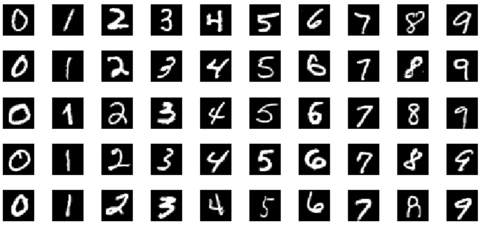
from Special Database 1 (SD-1). The testing set contains 10000 patterns, 5000 from SD-3 and 5000 from SD-1. All the patterns in the training set are developed by approximately 250 writers; and, the testing sets were developed by different writers. All the samples are normalized to fix-size (20 by 20 pixels) images and centered in 28 by 28 pixels planes. MNIST is a benchmark database for handwritten digit recognition and has been widely used to evaluate classifiers’ performances for over a decade [35]. Figure 3 displays some randomly selected images from the training set of MNIST, and some state-of-the-art recognition and rejection results on the MNIST isolated numerals database are listed in Table 1.

Figure 3. Image samples from MNIST handwritten digit database Table 1. Selected testing results on MNIST database

Method Distortion Error (%) Reject (%)

Boosted LeNet4 [20] Affine, scaling, squeezing 0.70 0.0

KNN [36] Non-linear deformation 0.52 0.0

TFE-SVM [25] Affine 0.54 0.0

CNN [24] Elastic 0.40 0.0

CNNs[37] Elastic 0.39 0.0

MCDNN [28] Width normalization 0.23 0.0

Cascaded CNNs [29] Elastic, scaling , rotating 0.23 0.0 Hybrid CNN-SVM [30] Elastic, scaling, rotating 0.19 0.0 Hybrid CNN-SVM [30] Elastic, scaling, rotating 0.00 5.6

(27)

19 (2) CENPARMI database [5]

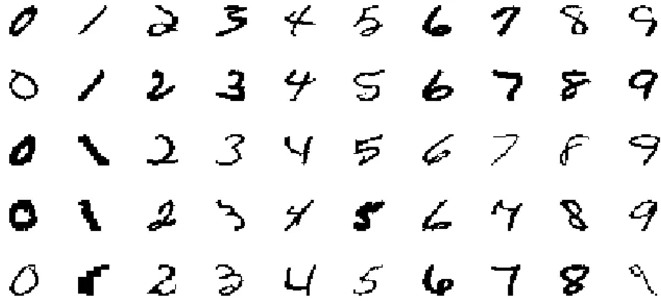
The CENPARMI handwritten digit database was assembled from U.S. ZIP code database of CENPARMI lab based at Concordia University. It contains approximately 17000 run-length coded binarized digits with an estimated number of 3400 writers. Samples are all unconstrained handwritten numeral images collected from dead letter envelopes, known as undeliverable mail, by the U.S. Postal Service which are then scanned in 166 PPI. In the CENPARMI database, there are 4000 images (equal number for each class of 0-9) used for training and 2000 (equal number for each class of 0-9) used for testing. All the images are of different sizes. Figure 4 displays some samples from the training set and Table 2 provides some sources of high accuracy on this database.

Figure 4. Image samples from CENPARMI handwritten digit database Table 2. Selected testing results on CENPARMI database

Method Error (%) Reject (%)

4-expert system[5] 0.0 6.95

multiple- expert system [38] 1.15 0.0

LQDF [8] 0.95 0.0

SVC-rbf [8] 0.95 0.0

8-direction, SVC-rbf [9] 0.85 0.0

(28)

20 (3) USPS database [6, 39]

USPS digits data was gathered as part of a project sponsored by the United States Postal Service. Digital images found in this database included approximately 500 city names, 5000 state names, 10000 ZIP Codes, and 50000 alphanumeric characters. They were scanned from mails in a working post office at 300 PPI in 8-bit grayscale [6]. This database was traditionally used in a splitting of 7291 samples for training and 2007 samples for testing (Version 1, referred to as V1). However, these two sets were actually collected in slightly different ways and samples in the testing set were much harder to classify than the ones in the training set. Hence, it was not very suitable for demonstrating learning algorithms. From there, all the samples from both training and testing sets were gathered and reshuffled to divide anew into training and test sets, containing 4649 samples each (Version 2, referred to as V2). All the 9298 digits images of USPS handwritten digit data have a fixed size of 16 by 16 pixels. Randomly selected samples from this database are displayed in Figure 5 while Table 3 lists selected previous recognition results.

(29)

21

Table 3. Selected testing results on USPS database

Method No. version Error (%) Reject (%)

Tangent Distance, 1-NN [40]* 1 2.5 0.0

Boosted Neural Network [41]* 1 2.6 0.0

LeNet1[42] 1 4.2 0.0 RVM [43] 1 5.1 0.0 GMD, VTS, TD [44] 1 2.7 0.0 KD, VTS, TD, Bagging [44] 1 2.2 0.0 SVM-rbf, e-grc3 [45] 1 2.39 0.0 SVM-rbf, e-grc3 [45] 2 1.33 0.0

*: training set extended with 2400 machine-printed digits

2.4 Distortion Methods

The CNN classifier is very powerful at classifying visual patterns, as it continues to yield state-of-the-art performances on visual analysis tasks. In order to further improve its recognition performance, especially in the cases where the numbers of training samples are small or the distributions have some transformation-invariant attributes, producing new samples to expand the datasets through transformation methods is feasible [24, 25]. Brief descriptions of two types of transformation methods are presented as follows:

(1) Affine distortion [25]

Affine distortion is a simple way to expand the dataset. It applies affine displacement fields to images in order to conduct the procedures of transformation including rotation, scaling and skewing. It is implemented by computing each pixel displacement fields, and , to locate the target position. The general form of affine distortion is:

(30)

22

where A is a 2*2 matrix and B is a column vector, storing parameters for transformation. For instance,

and are for scaling.

(2) Elastic distortion [24]

Elastic distortion is another transformation method introduced by Simard et al [24]. Within this transformation method, random displacement fields are first generated as shown in Eq. (9):

(9) where is a random number between and , generated by a uniform distribution. Then, and are convolved with a Gaussian standard deviation which stands for the elastic coefficient. A small means more elastic distortion while a large makes deformation approach affine. After that, the field values are normalized and multiplied by a scaling factor , controlling the intensity of deformation. Finally, the displacement fields are applied to each pixel of the image.

This elastic distortion method is adopted for dataset expansion for the process of MCS generation with dataset re-sampling method. Randomly selected samples from the training set are distorted with this method to generate new samples in order to form a new training set.

(31)

23

Chapter 3: Learning-based Rejection Criteria

Our main goal in this chapter is to improve the reliability of the single classifier by detecting error-prone samples and eliminating them from the testing process. To accomplish this, we have designed two novel rejection criteria, named SVM-based Measurement (SVMM) and Area Under the Curve Measurement (AUCM). The main difference between these two and other traditional rejection criteria is that they are learning-based criteria which extend the rejection process from heuristic design to learning procedure with training data. To evaluate the effectiveness of rejection, we can draw a Receiver Operating Characteristics (ROC) graph [46] in the coordinate system whose -axis is the number of rejected samples and -axis is reliability. A good rejection criterion can achieve a higher reliability with fewer samples rejected, so the curve is expected to be as close to the top left corner as possible. While the ROC curve will be introduced in Section 3.1, detailed designing ideas and architectures of SVMM and AUCM will be discussed in Sections 3.2 and 3.3 respectively. Both of these two novel rejection criteria will be compared with their traditional counterparts such as FRM, FTRM and LDAM through experiments on the MNIST database with the chosen CNN model.

3.1 Introduction of ROC analysis

A receiver operating characteristics (ROC) graph is used for visualizing, organizing and selecting classifiers based on their performance. It has a long history of usage in a variety of categories such as signal detection, visualizing and analyzing

(32)

24

diagnostic systems, medical decision making, etc. It is first adopted in the field of machine learning by Spackman in 1989 to evaluate and compare different algorithms [46].

ROC graphs are two-dimensional, depicting relative tradeoffs between benefits and costs. In the case of pattern rejection, there is always a tradeoff between two factors: the number of rejected samples and the reliability of the system. That is because reliability increases whenever confusing samples are rejected at early stages. In previous research of pattern rejection, reliability is always considered individually to evaluate a criterion’s effectiveness. However, it is insufficient to evaluate rejection performance based on this factor exclusively since it cannot be determined which method is superior in rejection if their reliabilities are based on different numbers of rejected samples. A system with low reliability based on few rejected samples may achieve very high reliability once the rejection rate increases. As a result, these two factors are supposed to be considered simultaneously to evaluate the performances of rejection systems and that is why we introduce the ROC curve for pattern rejection.

The ROC space is a two-dimensional coordinate system whose -axis and -axis represent the number of rejected samples and reliability, respectively. For a rejection criterion, there is always an output value and by setting thresholds for this value, it is decided whether a sample should be rejected or accepted. If different thresholds are set and rejection procedures are conducted accordingly, we can obtain a pair consisting of the number of rejected samples and corresponding reliability for each threshold. These pairs can be presented in the created ROC space as single points and

(33)

25

a smooth curve joining all of them (referred to as a ROC curve) represents the performance of the rejection criterion. A good rejection criterion can achieve a higher reliability with fewer samples rejected. So, we expect a good ROC curve to be as close to the top left corner as possible. This ROC curve will be used as a tool to evaluate all the proposed rejection criteria throughout the thesis.

3.2 SVM-based Measurement (SVMM)

3.2.1 Architecture of SVMM

Pattern rejection can be viewed as a two-class recognition problem, taking the classifier’s output values as features in order to recognize a pattern for rejection or acceptance. The traditional rejection criteria discussed in Section 2.2 have been designed based on some heuristic ideas. In this section, we propose a novel SVMM to extend the rejection process into a learning-based method.

Specifically, rejection can be viewed as a two-class recognition problem, one stands for rejected samples and the other for accepted ones. In SVMM, the classifier selected is SVM and the input is the output vector (always confidence values for possible classes) of a certain classifier. For a classifier, the output of a sample is a vector of confidence values , as mentioned before. Then, these values are used as features and sorted into a descending order:

The correctly and incorrectly classified samples are labeled differently: correctly classified samples are labeled with "1" while incorrectly classified ones are labeled

(34)

26

with "-1". This information is then used to train an SVM classifier. Linear SVM is selected for training in order to locate the rejection boundary. Therefore, the decision boundary is a linear function combining all the components of the output vector, represented in Eq. (11), where are the coefficients of SVM:

The reason for choosing a linear kernel for SVM rather than a nonlinear one, such as RBF kernel, is based on the following reasons:

(1) A linear kernel works very fast in training and testing, and an optimal linear separating boundary is a good way to avoid over-fitting.

(2) A linear boundary is more meaningful physically and function Eq.(11) includes some special cases in it. For instance, FRM can be viewed as a linear boundary with and ; while FTRM can be viewed as: and

.

Note that in the training process of SVMM, the number of samples in class "1" is always much larger than that of class "-1", because the baseline accuracy of the classifier is high. In this case, the problem is an unbalanced classification problem. To solve this problem, we use different weighting functions for different classes in the "libsvm" software [47]. In the testing process, the same features are extracted and sorted in descending order, and a sample is rejected if the calculated in Eq. (11) for it is smaller than a pre-defined threshold. Figure 6 is a flow chart depicting the whole rejection process:

(35)

27

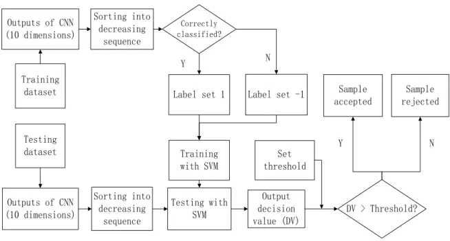
Figure 6. Flow chart of SVM-based Measurement (SVMM)

With this new criterion, the linear rejection boundary is found by training an SVM with the training set. The main difference between SVMM and other criteria, like FRM, FTRM and LDAM, is that SVMM extends the rejection process from heuristic design to a learning-based procedure. Using the learning-based method with training set to predict the rejection decision on testing samples is more straight-forward and allows researchers to use more information from the data.

3.2.2 Experiment with SVMM

In the selected CNN model presented in Section 2.2 (referred to as "M0"), the output of each sample is a 10-dimensional vector consisting of confidence values for the 10 possible classes. FRM, FTRM and LDAM are used respectively as rejection criteria with this basic model. Thresholds are searched incrementally. As in CNN model, the outputs are confidence values instead of probabilities, the most appropriate starting point, step and ending point for thresholds searching vary according to

Training dataset Outputs of CNN (10 dimensions)

Label set 1 Label set -1

Training with SVM Correctly classified? Y N DV > Threshold? Set threshold Sample rejected Sample accepted Y N Sorting into decreasing sequence Testing dataset Outputs of CNN (10 dimensions) Sorting into decreasing sequence Testing with SVM Output decision value (DV)

(36)

28

different rejection criteria. The search steps for them are all 0.1 at regular intervals and 0.01 at the sections where the number of rejected samples changes sharply.

Figure 7. ROC curves of SVMM and other rejection criteria with classifier "M0" For the newly proposed SVMM, "libsvm" tools are applied and the same CNN model "M0" is used as a feature extractor. Out of 60000, there are 216 samples labeled “-1” while the rest are labeled “1” for the training process. Since the training set is relatively unbalanced with the number of samples in class "1" at almost 300 times that of class "-1", the weight parameter is set to "400" for class "-1". A linear kernel is selected in order to find a linear decision boundary in the feature space. Normalization is conducted on the decision value with SVM of each sample with the purpose of making the threshold-setting procedure more convenient. Then, different thresholds are set for rejection. Since the output is a normalized value, the starting and ending points for threshold searching are 0 and 1 respectively while the search steps are 0.1 at regular places and 0.01 at the sections where the number of rejected samples fluctuates sharply. All the results are shown by the ROC curves presenting the

(37)

29

relationship between the number of rejected samples and reliability in Figure 7.

3.2.3 Comparison with other Rejection Criteria

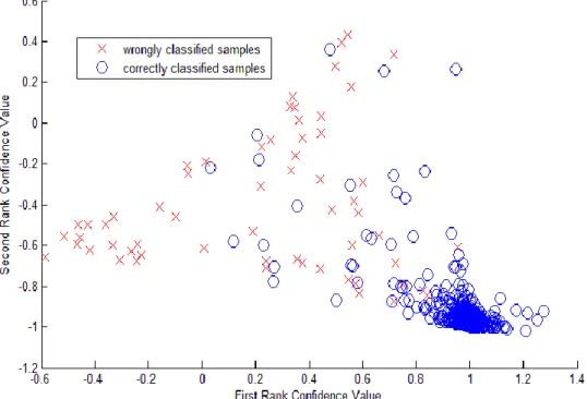
Although LDAM is proven to have a better performance than FRM and FTRM in He et al’s research [31] based on eight-direction gradient features with an SVM classifier; the results demonstrate that LDAM is the least useful one in our experimentations with the CNN model. As for FRM and FTRM from He’s work, their performances varied and yet, they are very similar when applied to the CNN model “M0”. Therefore, it can be concluded that these pre-defined criteria vary in performance with different classifier models or types of features. In Figure 8, some randomly selected samples from the training set are displayed in a 2-dimensional coordinate system based on their first two rank confidence values (FR and SR).

Figure 8. Samples in FR-SR feature space

(38)

30

1 and -1 respectively. As a result, a line with slope "1" standing for FTRM in the coordinate system is an optimal boundary to separate wrongly and correctly classified samples. That is why FTRM is an effective criterion in this model. Another effective criterion, FRM, can also be viewed as a way of finding a boundary parallel to the -axis, which is less effective than FTRM through observations. However, it is noticed that although these two criteria can be useful, many correctly classified samples will also be rejected by them no matter where the boundary is.

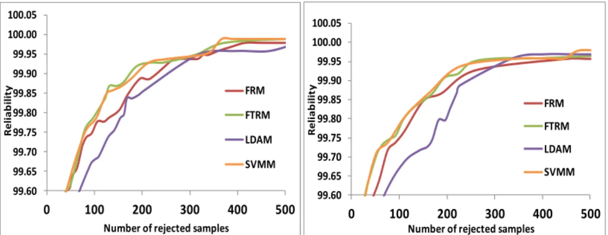
It is also shown in Figure 7 that SVMM works as effectively as FTRM in rejection and their performances are too close to determine which one is better. The same work has been completed with two other CNN models whose structures are similar to "M0". These CNN models produced only small changes in the number of maps in feature map layers. The results of these two models are displayed in Figure 9. It is apparent that SVMM and FTRM are always the relatively best ones among all of the rejection criteria. The reason behind the performances can be traced back to the training process of CNN model where the expected values in the decision layer are set to be "1" for the true class and "-1" for the other classes. Hence, FTRM is already a distinctively effective criterion to determine the quality of a sample as analyzed with Figure 8. When we use the SVMM, which uses all the values of the output vector, FR and SR contribute much more than the other eight confidence values since the others are slightly different from SR. Therefore, the rejection boundary of SVMM is very close to that of FTRM, explaining why these criteria display similar performances. In addition, despite the presence of a weight parameter for the class of rejection in

(39)

31

SVM training, the unbalanced data remains a critical factor affecting SVMM’s overall performance.

Figure 9. ROC curves of different rejection criteria with other CNN models

3.3 Area Under the Curve Measurement (AUCM)

3.3.1 Algorithm of AUCM

AUC, the name given to the novel rejection criterion, is the abbreviation of the expression: “area under the curve”. It is mentioned previously in Section 3.1 that in order to evaluate the effectiveness of a rejection criterion, we can draw a ROC curve in the coordinate system whose -axis represents the number of rejected samples whereas -axis represents the reliability. A good rejection criterion can achieve a higher reliability with fewer samples rejected, hence we expect a good curve to be as close to the top left corner as possible. In other words, we expect a good rejection criterion to make the area under this ROC curve to be as large as possible. To accomplish this goal, we attempt to determine a linear combination of FR and SR as a rejection criterion based on all training samples, because FR and SR are the most meaningful ones among all these confidence values.

99.60 99.65 99.70 99.75 99.80 99.85 99.90 99.95 100.00 100.05 0 100 200 300 400 500 Reli a b il it y

Number of rejected samples FRM FTRM LDAM SVMM 99.60 99.65 99.70 99.75 99.80 99.85 99.90 99.95 100.00 100.05 0 100 200 300 400 500 Reli a b il it y

Number of rejected samples FRM FTRM LDAM SVMM

(40)

32

Firstly, we create a linear combination of FR and SR, as followed in Eq. (12):

where , , and and are two parameters that will be derived from the training data to maximize the area under the ROC curve. Specifically, we simply fix the value of at “1” and search different values for . For each , there is a combination where

is the outcome. Pairs of number of rejected samples and reliability are calculated individually based on different thresholds of and displayed as single points in the ROC space. Then, a ROC curve is formed by connecting all the single points smoothly.

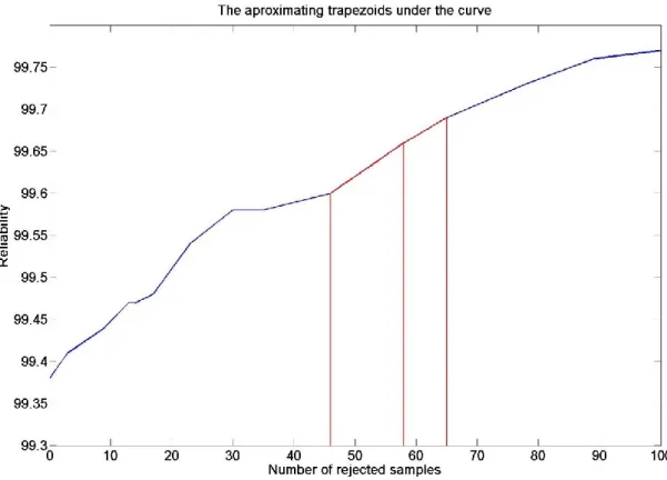
In order to compute the area under this curve, we approximate it by the sum of hundreds of small trapezoids as shown in Figure 10. The segmentation of the small trapezoids is based on the thresholds. For each combination of , rejection decision values of all the training samples can be calculated in order to find out the maximum value and the minimum value. Subsequently, the space between these two is divided equally into 200 parts, each of which is set as a threshold incrementally and used to generate a small trapezoid. The two parallel sides are the reliability values with the current threshold and its previous one. The height is the absolute difference between the number of rejected samples based on the current threshold and its previous one. Then, the area of the trapezoid for each threshold is calculated and the area under the curve can be computed accordingly by summing all of the small trapezoids. The areas under the curve of different s are compared to find out the maximum one in order to

(41)

33 obtain the best .

In the testing process, with the optimal , the responding combination is adopted as rejection criterion for the testing samples. A sample is rejected if its rejection value of is smaller than a pre-defined threshold.

Figure 10. The approximating trapezoids under the curve

3.3.2 Experiment with AUCM

This AUCM rejection criterion is also evaluated with CNN model “M0” on MNIST database. As mentioned in Section 3.3.1, is fixed at “1”. The is searched from “-5.0” with an incremental step of “0.05” until “5.0”. For each pair, the area under the curve is calculated through the approximation of the sum of hundreds of small trapezoids under it, as discussed in Section 3.3.1. The optimal searched out to maximize the area under the ROC curve is “-1.75” in our experiment. So, the rejection criterion is determined to be:

(42)

34

A sample is rejected if its rejection decision value in Eq. (13) is smaller than a threshold.

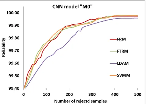
Figure 11. ROC curves of AUCM and other rejection criteria with classifier "M0"

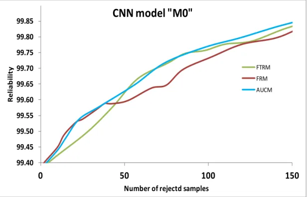
In the testing process, because the range of the output values varies according to the different combination Ts, the starting and ending points for threshold setting remain unstable. So, we first look for the maximum and minimum values for a specific to determine the starting and ending points. In this experiment, the starting point is -0.4 and the ending point is 2.7. The search steps for the threshold are still 0.1 at regular places and 0.01 at the sections where the number of rejected samples fluctuates sharply. The rejection result of AUCM is shown in Figure.11 with those of FRM and FTRM, as ROC curves illustrating the relationships between the number of rejected samples and reliability.

99.40 99.45 99.50 99.55 99.60 99.65 99.70 99.75 99.80 99.85 0 50 100 150 Rel ia b il it y

Number of rejectd samples

CNN model "M0"

FTRM FRM AUCM

(43)

35

3.3.3 Comparison with other Rejection Criteria

It is clearly indicated from Figure 11 that the AUCM achieves a higher performance than the other two criteria, because its ROC curve is closer to the left-top corner and remains higher than those of FTRM and FRM in almost its entire path. It means that with AUCM, we can always obtain a higher system reliability when compared with FTRM and FRM based on the same number of patterns rejected. It proves the effectiveness of this new rejection criterion.

The advantage of AUCM can be explained from its designing idea of finding the optimal combination of FR and SR as a rejection criterion from the training data. This information is then interpreted as finding the best combination to maximize the area under the ROC curve, which is applied to evaluate the rejection criterion’s performance. In the parameters searching process, the coefficient of FR ( ) is fixed at "1" and that of SR ( ) varies between "-5" and "5", which includes the FRM and FTRM as special cases of the combinations ( for FRM and

for FTRM). Therefore, the combination with the optimal and pair works more effectively than FRM and FTRM based on the training set, since its area under the curve is the largest among all including those of FRM and FTRM. Generally, it is assumed that the training and testing sets are closely related; hence demonstrating that the optimal combination on the training set is supposed to achieve a better performance on testing set. Later, this assumption is proven by the experimental result that the optimal combination of FR and SR on the training set works more effectively than other criteria on the testing set as well.

(44)

36

Chapter 4: Rejection with MCS

In this chapter, the Multiple Classifier System (MCS) will be studied for the purpose of pattern rejection which is implemented by using voting methods to combine decisions from different single classifiers. The CNN classifier "M0" [30] will still be used as a basic model. To construct the committees of a MCS, two simple methods including dataset re-sampling (DR) and structure modification (SM) are chosen. The details on how the MCSs are constructed will be described in Section 4.1. Section 4.2 will provide the proposed voting-based combination methods’ algorithms. Both hard voting and soft voting will be considered. In Section 4.3, the new MCS based rejection method will be evaluated on three notable handwritten digit databases: MNIST, CENPARMI and USPS. All the experimental results and analyses will also be displayed in this section.

4.1 Construction of MCS

Re-sampling the dataset (with Bagging [48], Boosting [49] and so forth) and changing the classifier (in structure or type [50]) are two main ways to produce committees of MCSs. Many researchers have used these methods to produce a group of classifiers and applied certain combination methods for recognition. On the other hand, CNN classifier, especially MCS based on CNN, works extremely effectively in handwritten character recognition [28, 29, 30]. Therefore, the CNN model "M0" is selected as the core classifier and both of the two methods, dataset re-sampling (DR)

(45)

37

and structure modification (SM), are adopted to build MCSs according to our strategy. As seen in Chapter 2, our CNN model "M0" has 2 feature map layers and 1 hidden layer with 25, 50 and 100 feature maps respectively to store the features after convolutional filtering and they are named as F1, F2 and F3. Two types of modifications have been explored: one is by adding or subtracting the numbers of feature maps in each of the three feature map layers; the other is using "Bagging" method, such as dataset re-sampling, to randomly select samples from the training sets to train the same CNN model numerous times.

(1) MNIST

For the MNIST database, SM method is initially applied to build committees. We alter the model's structure slightly by increasing and decreasing the number in each feature map layer. Specifically, there are six modified structures ("M1" to "M6"), as shown in Table 4 below. In order to diversify recognition results, we change the number of feature maps in one of these layers and keep the rest intact every time. In M1 and M2, we merely change F1, in M3 and M4, we change F2, and in M5 and M6, F3. Then, all of the models are trained to the 500th epoch until the recognition rates of the training set remain stable. All the error rates, generated from the testing loops, are listed in Table 4.

After that, the model structure is fixed at "M0" and DR is adopted to generate the committees. It is noted that 30000 samples, which represent half of the samples in the training set, are randomly extracted for each committee. The elastic distortion algorithm [24] is then implemented to produce 30000 new

(46)

38

samples with parameters and . Some samples as well as their distorted counterparts are presented in Figure 12. Afterwards, these two groups of samples are merged to form the new training set with 60000 samples. This procedure is repeated five times to create five distinct training datasets while the "M0" is trained on them respectively to build a MCS with five committees ("G1" to "G5"). The information of each re-sampled training set is listed in Table 5 along with their recognition error rates based on the MNIST testing dataset at the 300th epoch of training when the recognition rates achieve stability.

Table 4. Information about SM in MCS on MNIST database

M0 M1 M2 M3 M4 M5 M6

F1 25 25 25 25 25 10 40

F2 50 50 50 30 80 50 50

F3 100 80 120 100 100 100 100

Training Error Rate (%) 0.36 0.34 0.31 0.34 0.26 0.34 0.29 Testing Error Rate (%) 0.62 0.63 0.61 0.60 0.58 0.63 0.61

Table 5. Information about DR in MCS on MNIST database

G1 G2 G3 G4 G5 0 2938 2936 2945 2940 3009 1 3467 3412 3399 3339 3420 2 3008 2936 3026 2953 2939 3 2959 3083 3055 3105 3028 4 2895 2866 2850 2996 2803 5 2672 2745 2700 2676 2788 6 2990 2982 2946 2996 3031 7 3144 3076 3165 3060 3137 8 2906 2965 2992 2987 2954 9 3021 2999 2922 2948 2891

Training Error Rate (%)

of re-sampled dataset 0.79 1.10 1.11 1.43 1.10

of original dataset 0.68 0.76 0.72 0.83 0.74

Testing Error Rate (%) 0.60 0.73 0.75 0.79 0.71

(47)

39

Figure 12. Samples from MNIST database and their distorted counterparts (2) CENPARMI

For the CENPARMI database, we start by increasing the numbers of feature maps in each feature map layer (F1, F2 and F2) of the "M0" while training all the models to the 150th epoch when the error rates remain stable, as shown in Table 6, to construct the MCS.

Table 6. Information about SM in MCS on CENPARMI database

M0 (basis) M1 M2 M3

F1 25 50 50 70

F2 50 75 90 75

F3 100 120 100 100

Training Error Rate (%) 0.50 0.38 0.38 0.43

Testing Error Rate (%) 2.45 2.45 2.25 2.45

Table 7. Information about DR training sets on CENPARMI database

G1 G2 G3 G4 0 474 450 458 402 1 462 408 482 440 2 416 358 408 380 3 350 404 340 390 4 332 394 372 430 5 394 382 410 426 6 380 424 392 370 7 370 424 426 412 8 400 396 386 350 9 422 360 326 400

of re-sampled dataset 1.65 1.52 1.27 1.77

of original dataset 1.42 1.78 1.9 1.4

(48)

40

DR method is then used to build the MCS. During this phase, model structure is fixed as the basic one. Different training sets are formed by randomly selecting 2000 training samples and distorting them with elastic distortion algorithm [24] using the same parameters as in MNIST ( and ). The process is repeated four times to obtain four different training sets (G1-G4) with 4000 samples each, as seen in Table 7 alongside with recognition results on the testing set after 150 epochs when the error rates get stable.

(3) USPS

For the USPS database, there are two versions including one with 7291 training samples and 2007 testing samples (referred to as V1) and the other version with 4649 samples for each of the two sets (referred to as V2).

Firstly, we increase the amount of feature maps in each feature map layer (F1, F2 and F3) of the "M0" to build “M1” to “M3”. All the models are trained for 300 epochs until the recognition rates on training set achieve stability. This work is completed for both of the two versions of USPS database and the results are shown in Table 8.

Table 8. Information about SM in MCS on USPS database

M0 M1 M2 M3

F1 25 40 25 25

F2 50 50 80 50

F3 100 100 100 120

Training Error Rate (%) on V1 2.15 2.13 2.08 2.07

Testing Error Rate (%) on V1 3.84 4.04 3.89 3.99

Training Error Rate (%) on V2 2.41 2.54 2.58 2.47

(49)

41

Table 9 (a). Information about DR training sets on USPS database (V1)

G1 G2 G3 G4 0 600 621 606 617 1 487 460 505 494 2 378 373 371 351 3 324 299 327 332 4 347 326 355 342 5 276 295 267 269 6 321 311 310 311 7 311 311 303 321 8 291 302 273 284 9 310 347 328 324

Training Error Rate of

5.47 4.75 4.66 4.65

re-sampled dataset on V1(%) Training Error Rate of

re-sampled dataset onV1 (%) 3.74 3.32 3.51 3.51

Testing Error Rate on V1 (%) 4.63 4.93 4.83 4.98

Table 9 (b). Information about DR training sets on USPS database (V2)

G1 G2 G3 G4 0 365 380 393 398 1 301 295 275 290 2 240 220 254 248 3 194 231 219 195 4 229 187 197 209 5 193 164 164 175 6 215 21