The implementation of monetary and fiscal rules in the EMU: a welfare-based analysis

(1)

FIW, a collaboration of WIFO (www.wifo.ac.at), wiiw (www.wiiw.ac.at) and WSR (www.wsr.ac.at).

FIW – Working Paper

The implementation of monetary and

fiscal rules in the EMU:

a welfare-based analysis*

Amedeo Argentiero

This paper implements a methodology to evaluate the desiderability of monetary

and fiscal rules within the context of the EMU using a DSGE model within a New

Keynesian framework with sticky prices. The approach adopted is a

welfare-based criterion that measures the welfare losses associated with these rules

through a welfare loss function. Monetary policy follows a standard Taylor rule

augmented by a stochastic component, driven by a union-wide monetary shock,

whereas fiscal policy is made up of a countercyclical and debt-stabilizing public

expenditure and of distortionary taxation on labor, dividends and interests on

public bonds.

We find that: 1) in the presence of our monetary rule alone, domestic inflation

variance falls more than in the only presence of fiscal rules, whereas output gap

smoothing is stronger in the only presence of fiscal rules; 2) the combination of our

monetary rule and fiscal rules reduces welfare losses more than the same rules

singly considered.

JEL classification:

E63, F41, E32;

Keywords:

Fiscal Rules, Monetary Rule, Feedback-on-Debt, Welfare

Losses;

Amedeo Argentiero

is researcher at the University of Rome Tor Vergata as well as at

the Institute for Study and Economic Analysis (ISAE).

E-Mail:

[email protected]

or

[email protected]

* The author is very grateful to Francesco Nucci for his supervisor activity, to Patrizio Tirelli, Fabrizio Mattesini, Pierpaolo Benigno and Fabio Cesare Bagliano for their very useful comments. He would like to thank the Department of Economics of University of Rome Tor Vergata and the Italian Ministry of Economy and Finance for their financial support for this research project. He would like to thank Gustavo Piga, Paolo Paesani, Rita Ferrari, Mario Tommasino, Paolo Biraschi, Juan J. Pradelli, Alessandra Pelloni, Alessandro Girardi, Rafaella Basile, Gabriele Velpi and Guido Lorenzoni for many conversations and precious advice. He also thanks the participants of XVI International Tor Vergata Conference on Banking and Finance, of the First Italian Doctoral Workshop in Economics and Policy Analysis of Collegio Carlo Alberto and of the second FIW Research Conference on "International Economics" in Vienna for comments on previous versions of the paper.

Abstract

The author/s

FIW Working Paper N°33

(2)

(3)

1

Introduction

The Stability and Growth Pact (henceforth SGP) with its budget rules repre-sents a sort of ex-post …scal coordination mechanism for EMU countries, where there is the "cohabitation" of one independent monetary policy and many …scal policies. The aim of these …scal rules is to stabilize Public Debt with respect to GDP, through the control of de…cit with respect to GDP, both in the short term and in the medium term. In words, the SGP is founded on the idea that excessive de…cits and high debts with respect to GDP are able to destroy the economic architecture of the EMU.

A large part of the literature (Buti et al. (1997), Melitz (2000), Wyplosz (2002), Galì and Perotti (2003)) has developed di¤erent works to understand whether the SGP has tied the EMU members’hands in pursuing the stabiliza-tion of the business cycles through the instruments of …scal policy (i.e. taxastabiliza-tion and public expenditure). Nevertheless, evidence is not univocal and covers a very short time span (at the most ten years) for the construction of a represen-tative sample in the EMU that incorporates di¤erent scenarios for the business cycle and the application of …scal policy instruments to it.

Buti et al. (1997) underline an excessive procyclicality for …scal policy in EMU countries during and after severe recessions in the period 1961-1996; Melitz (2000) …nds strong evidence of stabilization for the ratio Debt/GDP in EMU countries, but …nds a weaker stabilizing movement for public expenditures; Wyplosz (2002) …nds evidence for Italy, France and Germany of a countercycli-cality in public consumption and an acyclicountercycli-cality (Italy) or procyclicountercycli-cality (France and Germany) for tax revenues. Anyway for the years 1992-20011_{he …nds some}

evidence of an asymmetric behavior of …scal policy components: in France there is a countercyclical reaction to downswings and a procyclical reaction to up-swings; in Italy, public expenditure is more countercyclical and taxation more procyclical during downswings. The study of the sub-sample 1992-2001 has been driven by a key question of a large part of literature: have the Maastricht convergence criteria and the SGP requirements weakened the stabilizing role of …scal policy in EMU countries? An attempt to answer this question, supported by a detailed empirical analysis, is given by Galì and Perotti (2003), who point out that …scal policy in the EMU has become more countercyclical over time, following what appears to be a trend that a¤ects other industrialized EMU and non-EMU countries as well; therefore, the SGP constraints would not represent an impediment on a stabilization path. Moreover, the decline in public invest-ment, observed in the recent data, seems to follow a common tendency in other countries and starts before the implementation of the SGP. However, as Galì and Perotti state, real recessions in the period after-Maastricht have been quite rare and hence the available data are not so binding to announce a "failure" in the stabilizing activity of …scal policy.

The goal of this paper is to evaluate, within a DSGE model, the performances of two …scal rules, the former on public expenditure and the latter on taxation,

(4)

and one monetary rule, i.e. a Taylor rule increased by a stochastic component driven by a monetary shock. Public expenditure follows a countercyclical and debt-stabilizing rule, whereas taxation is given by the sum of tax revenues com-ing from distortionary taxation on labor, on dividends and interests on public bonds issued by the government to …nance its stock of debt. In this way, pub-lic expenditure pursues both the objectives of debt stabilization, as imppub-licitly required by the SGP from …scal policy, and business cycle stabilization, that is one of the purposes assigned to …scal policy (Musgrave (1959))2_.

Our analysis makes use of a microfounded theoretical New-Keynesian model with sticky prices à la Calvo (1983) applied to a currency union, following a large body of literature (Beetsma and Jensen (2005), Ferrero (2005), Galì and Mona-celli (2008), Colciago et al. (2008) among others), and a welfare loss function for each country belonging to the currency union to compute the consumers’losses in the presence of monetary and …scal rules. This approach has been imple-mented by much literature for monetary policy rules (Rotember and Woodford (1999) and Galì (2008) among others), relying on a second-order approximation to the utility losses of the households caused by deviations of variables from their e¢ cient allocation values. Also Ferrero (2005) uses a welfare-based approach to evaluate the desiderability of …scal and monetary rules in a currency union, his analysis di¤ers from ours essentially for the presence of a rule on real stock of public debt instead of a rule on public consumption as we do and for the use of a di¤erent welfare loss function. Indeed, Ferrero (2005) uses Benigno and Woodford’s (2005) welfare loss function, that is able to take into account the presence of distortionary taxation and a positive stock of debt with correspond-ing steady state values di¤erent from the ones of the Central Planner’s solution. The welfare loss function adopted in this paper, instead, has the same structure as the one of Galì and Monacelli (2008)3_{: the arguments of this function are the}

squared domestic in‡ation, the squared output gap and the squared …scal gap4_.

The benchmark value of these variables against which we measure the losses is represented by a fully ‡exible prices equilibrium with lump-sum taxation able to …nance public consumption, whose optimal behavior is described in the Ap-pendix, in the absence of public debt and any rules on monetary policy. In such a framework the fully ‡exible prices equilibrium calculated as the solution of

2_{This theory designs three purposes for …scal policy and it also does the same for public} expenditure: the provision for social goods, i.e. theallocation function of budget policy; the distribution of wealth among the citizens to equalize the incomes, i.e.the distribution function

and the business cycle stabilization, i.e. the stabilization function.

3_{Galì and Monacelli (2008) show that, in the presence of sticky prices, the combined} monetary-…scal policy mix able to maximize the average welfare of union households must leadat the union levelto a constant (zero) value both for the output gap, in‡ation and …scal gap. Anyway, the same authors argue that the union-wide equilibrium in general cannot be an equilibrium under the optimal policyfor each member country: in this case the second-best allocation of the in‡ation gap and the output gap will have a non trivial equilibrium dynamics as for the union level. This equilibrium dynamics can be described through a series of dynamics simulations, given an appropriate calibration for the model parameters.

4_{Fiscal gap is de…ned as the share of output used for public consumption less the amount} of public expenditure to which the households give a weight in the utility function.

(5)

the Social Planner’s problem is also supported at a decentralized level5. In particular, we compare three di¤erent scenarios: in the …rst one there is the only presence of our monetary rule with lump-sum taxation able to …nance public consumption at its optimal level, and in the absence of public debt; in the second scenario there are only …scal rules and no monetary policy rules, whereas in the third scenario both …scal and monetary rules are present.

Here is an overview of the results:

the presence of only our monetary rule is able to generate a stronger decrease in domestic in‡ation variance than the presence of …scal rules only;

the presence of our …scal rules generates an output gap smoothing stronger than our monetary rule alone;

the combination of monetary and …scal rules generates less welfare losses than the rules considered in isolation.

Hence, in the EMU the attainment of price stability should depend on the common monetary policy, whereas …scal policy, institutionally decentralized at a country level, should be focused on output gap stabilization, that, in turn, can be also reached in the presence of rules that ensure countercyclicality to …scal policy, together with debt stabilization, as required by the SGP.

The paper is organized as follows. The model structure and its properties are set out in section 2. In Section 3, we derive the equilibrium market clearing conditions for the demand side of the market and for the supply side; in section 4, we discuss the calibration of the model parameters, whereas in section 5 we analyse, through the impulse response functions, the results coming from the time series generated by the model both in the presence of a technology shock and a union-wide interest rate shock. In section 6, we conclude.

2

A Currency Union Model for Fiscal Policy

We develop a closed currency union model, in the spirit of Galì and Monacelli (2008), made up of a continuum of small open economies, represented by the unit interval, such as the domestic policy decisions do not have any e¤ect on the rest of the union.

We consider such a framework suitable to give a realistic description of the inner structure of a monetary union like the EMU, made up of …fteen members (each one with an independent …scal authority). In fact and in line with a small country model, EMU countries are small relative to the union as a whole. Hence, each country’s policy decisions have very little impact on the other countries; this context, as a matter of principle, could be described by widening the existing one to incorporate …fteen countries, but such undertaking would render the resulting model intractable.

(6)

In this model, each country has identical preferences, technology and market structure; three agents are considered within each economy: the households, the …rms and the government.

2.1

Households

All households living in the representative country i belonging to the monetary union aim to maximize an utility function de…ned over private consumption,

C_ti; hours of work,N_ti and public expenditureGi_t:

E0 1 X t=0 t_{U C}i t; Nti; Git (1) The consumption index Ci

t is de…ned as the Dixit-Stiglitz aggregator over the bundles of goods produced in country i andf respectively:

C_ti= C i i;t 1 m Ci F;t m (1 m)(1 m)mm (2)

whereC_i;ti is a Dixit-Stiglitz aggregator de…ned over the continuum of di¤erenti-ated goods produced in country i andj [0;1]denotes the type of good (within the set produced in country i). Each lot of goods is produced by a separate …rm and no goods are produced in more than one country:

C_i;ti = Z 1 0 C_i;ti (j) 1dj 1 (3) The aggregatorC_F;ti ;in turn, is an index of country i’s consumption of imported goods and represents an exogenous variable for country i:

C_F;ti = exp

Z 1 0

ci_f;tdf

where ci_f;t6 = logCf;t is the log of an index of the goods consumed by country i’s households that are produced in country f: This index is de…ned symmetrically to (3): C_f;ti = Z 1 0 C_f;ti (j) 1 dj 1

Note that in the speci…cation of composite consumption index above, m

[0; 1]is the weight of imported goods in the utility of private consumption; we can think atm as an index of openness. The parameter >1 is the elasticity of substitution across goods produced within one country.

6_{In what follows, all the variables in small letters indicate the logarithms of the} correspon-dent variables in capital letters.

(7)

The utility function takes the following form, following Galì and Monacelli (2008): Ui C_ti; N_ti; Gi_t = (1 ) logC_ti+ logGi_t N i(1+ ) t (1 + ) (4)

where parameter [0; 1)represents the preference for public consumption

Git.

All the prices are set in the common numeraire. The law of one price is assumed to hold, so that the price of each variety of goods is the same across countries. The implied overall consumption-based price index is:

P_c;ti = P_ti 1 m(P_t)m (5) where Pi t = R1 0 P i t(j)1 dj 1 1

represents country i’s domestic price in-dex (i.e., an inin-dex of prices of domestically produced goods), for all i [0;1]and

P_t = expR₀1pf_tdf is the union-wide price index, that from the viewpoint of any individual country can be seen as the price index for imported goods. Sym-metrically, the price index for the basket of goods imported from countryf is de…ned as P_tf = R₀1P_tf(j)1 dj

1 1

. Note that the elasticities of domestic price index and union-wide price index de…ned in (5) correspond to the relative weights of the respective goods in the consumption basket.

The maximization of (1) is subject to the following sequence of budget con-straints: Z 1 0 P_ti(j)C_i;ti (j)dj+ Z 1 0 Z 1 0 P_tf(j)C_f;ti (j)djdf+Et Qt;t+1 Bi;ti +1+ Z 1 0 B_f;ti ₊₁df+ i_i;t₊₁+ Z 1 0 i f;t+1df (1 n)WtiNti+Bi;ti + Z 1 0 Bf;ti df+ ii;t+ Z 1 0 i f;tdf ti (6) wherePi

t(j)is the price of the domestic goods (expressed in units of the single currency) andP_tf(j)is the price of the imported goods. Bi

i;tis the nominal value net from interest rate taxation in periodtof a bond issued by the government of countryi in period tand purchased by the citizens of country i, Bi

f;t is the nominal value net from interest rate taxation in periodtof a bond issued by the government of countryf in periodtand purchased by the citizens of country i:

B_i;ti = (1 #) 1 +r_t(1 k)Dti B_f;ti =#h1 +r_t(1 k)Dft i whereDi t D f

t is the nominal stock of public debt issued by the Government of countryi(f)and whose law of motion is discussed later, r_t is the nominal interest rate for the currency union, that follows a Taylor rule as explained in the next section, the fraction#(1 #)is the share of foreign (domestic) debt purchased by the households of countryi. i_i;tis the nominal dividend in period

(8)

t for a share7 of a domestic …rm purchased in t by the domestic households, whereas i_f;tis the nominal dividend in period t for a share of a foreign …rm purchased int by the domestic inhabitants:

i i;t+1= (1 ) (1 k) it (7) i f;t+1= (1 k) ft (8) where i t f

t is the nominal pro…t of the representative …rm of countryi(f), the fraction (1 )is the share of domestic (foreign) …rm held by each inhabi-tant of countryi. i

t denotes lump-sum taxes, whose role will be discussed later.

Wi

t is the nominal wage, nis a distortionary wage tax levied by the government on labor and k is a distortionary tax levied by the government on the income coming both from dividends and bonds, that are the …nancial assets of the rep-resentative consumer. Qt;t+1 is the stochastic discount factor for one-period

ahead nominal values of each …nancial asset: it is common across countries. For each country, household’s consumption must be optimally allocated across all di¤erentiated goods: expenditure on goodsjis negatively related to the relative price of goodsj and it satis…es the following …rst-order conditions:

C_i;ti (j) = P i t(j) Pi t C_i;ti ;C_f;ti (j) = P f t(j) P_tf ! C_f;ti (9)

for all i; f; j [0;1]. it follows from the previous relationship thatR₀1Pi

t(j)Ci;ti (j)dj=

P_tiC_i;ti andR₀1P_tf(j)C_f;ti (j)dj=P_tfC_f;ti :

For countryf symmetric conditions hold as for country i; in particular, the consumer price index (CPI) is thus obtained:

P_c;tf = P_tf 1 m(P_t)m (10) if we log-linearize and integrate both the members of the previous relation-ship overf [0;1], we obtain the equality (11):

p_c;t=p_t (11)

Moreover, the optimal allocation of expenditures for imported goods by country of origin implies:

P_tfC_f;ti =P_tC_F;ti (12) for allf [0;1]:

Finally, combining all the previuos results, we can express respectively the optimal allocation of expenditures between domestic and imported goods in

7_{In what follows, we suppose that the value of the shares held is given only by the value of} the dividends; the initial value of each share is zero and there is not any form of capital gain.

(9)

country i and the total consumption expenditures by country i’s households in the following way:

P_tiC_i;ti = (1 m)P_c;ti C_ti (13)

PtCF;ti =mPc;ti Cti (14)

P_tiC_i;ti +P_tC_F;ti =P_c;ti C_ti (15) Hence, the period budget constraint can be rewritten in a more compact way as:

P_c;ti C_ti+ (1 k)Et Qt;t+1Fti+1 (1 k)Fti+ (1 n)WtiNti whereFi

t is a portfolio that collects all the …nancial assets purchased by the domestic households.

The remaining optimality condition for the control variables(C_ti; N_ti)for the households are given by:

Cti Nti = (1 ) Wi t(1 n) Pi c;t (16) For each household, the optimality condition for the allocation of wealth among the …nancial assets characterizes the stochastic discount factor as:

( Ci t Ci t+1 Pi c;t Pi c;t+1 !) =Qt;t+1 (17)

if we take the expected value on both the members of (20), we obtain the standard form of the Euler equation:

Et " Ci t Ci t+1 Pi c;t Pi c;t+1 ! R_t₊₁ # = 1 (18) whereR_t₊₁= _E 1

tfQt;t+1g is the gross nominal interest rate.

The assumption of complete markets for the …nancial assets across the union implies for countryf an Euler equation analogous to (21):

Et " Ctf C_tf₊₁ ! P_c;tf P_c;tf₊₁ ! R_t₊₁ # = 1 (19)

Combining (18) and (19), we obtain:

C_ti= iCtf P_c;tf Pi c;t ! (20) where i = Pc;ti +1C i t+1

P_c;tf ₊₁Cf_t₊₁ is a constant which depends on initial conditions re-garding relative net asset positions: if we suppose zero net foreign asset holdings

(10)

for all countries together with the hypothesis of an ex-ante identical environ-ment, we have the case in which i= = 1 for alli [0;1], i.e.:

C_ti=C_tf P f c;t Pi c;t ! (21) Moreover, in each country government’s assets are also subject to the fol-lowing transversality condition:

lim T!1Et n Qt;T+1 h Bi_i;T₊₁+B_i;Tf ₊₁io= 0 (22) lim T!1Et n Qt;T+1 h Bf;Ti +1+Bf;Tf +1 io = 0 (23)

In the next subsection, we describe the behavior of the central bank, that determines the monetary policy for the currency area, using the short-term nominal interest rate as its main instrument, but, before this step, we de…ne the domestic CPI gross rate of in‡ation and the union-wide gross rate of in‡ation, respectively as: i c;t= Pi c;t Pi c;t 1 (24) t = P_t P_t ₁ (25)

2.2

Interest rate and monetary policy

The Central bank sets the short-term nominal interest rater_t for the currency union as a linear function of the the union-wide current in‡ation _t and the union-wide output gap, de…ned here as the deviation of outputy_t from its level under fully ‡exible price valuey_tn(Taylor rule). it is typically assumed that the coe¢ cient on in‡ation is greater than one8, which implies that the central bank raises the nominal interest rate more than one-for-one in response to an increase in in‡ation:

r_t =r + ( _t) + y(yt ytn) +$t (26)

The quantity $_t is an exogenous stochastic component, which follows the following omoschedastic white-noise process:

$t = $$t 1+"$t

we can think of"_$tas a monetary shock, whereasr is the steady-state level of long-term real interest rate, that can be derived from the Euler equation (21):

[ (1 +r )] = 1 (27)

r = 1 1 (28)

8_{This condition is in line with the …ndings of Bullard and Mitra (2001) and satis…es the so} called "Taylor principle".

(11)

2.3

Firms

Each country has a continuum of …rms represented by the intervalj [0;1]. Each …rm produces di¤erentiated goods with a linear technology:

Y_ti(j) =Ai_tN_ti(j) (29) where Ai

t is a country-speci…c aggregate technology index, whose law of motion follows an AR(1) process (in logs):

ai_t= aait 1+"iat (30) and af0;1g:Moreover, we suppose that the stochastic process, that gener-ates labor productivity is an omoschedastic white noise and it’s assumed a null correlation between the monetary shock and the technology shock.

The assumption of a linear technology implies that real marginal costs are given by:

mci_t= log 1 si +wi_t pi_t ai_t

where si _{is a constant empolyment subsidy with the role to o¤set …rms’} market power represented by the monopolistic competition. This subsidy is completely …nanced by the lump-sum taxes i

t as in the model of Galì and Monacelli (2008).

We assume a staggered price setting à la Calvo (1983). As in Galì (2008), there is a number1 of (randomly selected) …rms, which sets new prices each period, with an individual …rm’s probability of reoptimizing in any given period being independent of the time elapsed since its last price resetting. Hence, the parameter is an index of stickiness. The aggregate price dynamics is described by the following equation:

i(1 ) t = + (1 ) PiR t Pi t 1 1 (31) where i t= Pti Pi t 1

is the gross in‡ation rate andPiR

t is the price set in period t by …rms reoptimizing their price in that period. A …rm reoptimizing in period t chooses a pricePtiR that maximizes the current market value of the pro…ts it, by solving the following problem:

max PiR t 1 X k=0 k_E t n Qi_t;t₊_k P_tiRYt+kjt it+k Yti+kjt o (32) subject to the sequence of demand constraints

Y_ti₊_k_j_t= P iR t+k Pi t+k ! C_ti₊_k (33)

fork= 0;1;2; :::and whereQi

t;t+k= k Cti+k=Cti Pti=Pti+k is the discount factor, it( )is the cost function of the …rm, whereasYti+kjtrepresents output

(12)

in periodt+k for a …rm resetting its price in period t. Next, the …rst order condition associated with the problem (32) is given by:

1 X k=0 k_E t n Qi_t;t₊_kYt+kjt PtiR M ti+kjt o = 0 (34) where i t+kjt= 0_i

t+k Yti+kjt indicates the nominal marginal cost in period

t+k for a …rm resetting its price in period t andM = ₁9 _{is the optimal}

markup in absence of constraints on the frequency of price adjustment. Note that in the absence of price rigidities( = 0)the previous condition collapses to the optimal price setting condition under ‡exible prices:

P_tiR=M i_t_j_t (35)

Moreover, in this particular case, by setting si ₌ 1 _{and substituting this}

value and the de…nition of nominal marginal costs into (35), an optimal market allocation, that is able to completely eliminate the consequences of monopolistic competion, can be reached. In fact, ifsi ₌ 1_{, expression (35) turns into the}

optimality condition of perfect competition, according to which the price should be equal to the marginal cost.

Then, we divide both the members of (34) byPi t 1: 1 X k=0 k_E t Qit;t+kYt+kjt P_tiR Pi t 1 M M Ct+kjt it 1;t+k = 0 (36) whereM Ct+kjt= i t+kjt Pi

t+k is the real marginal cost in periodt+kfor …rms whose

last price set is in periodtand, …nally, we log-linearize the optimal price setting condition (36) around the zero in‡ation steady state with a …rst-order Taylor expansion: piR_t pi_t ₁= (1 ) 1 X k=0 ( )kEt h c mci_t₊_k_j_t+ pi_t₊_k pi_t ₁ i (37) where mc_ci_t₊_k_j_t = mci

t+kjt mc is the logdeviation of marginal cost from its steady state value.

The optimal price setting strategy for the typical …rm resetting its price in periodt can be derived from (37), reducing some algebra:

piR_t = + (1 ) 1 X k=0 ( )kEt h mci_t₊_k_j_t+pi_t₊_ki (38)

with = log ₁; that represents the optimal markup in the absence of constraints on the frequency of price adjustment( = 0): Hence, the price set-ting rule for the …rms resetset-ting their prices is represented by a charge over the

(13)

optimal markup in the presence of fully ‡exible prices, given by a weighted av-erage of their current and expected nominal marginal costs, with the weights being proportional to the probability of the price remaining e¤ective( )k. In a zero-in‡ation steady state equilibrium and in the absence of price stickiness for all the …rms( = 0);the previous expression collapses to:

pi = + 1 (39)

Note that, under the hypothesis of costant returns to scale, implicit in the production function of our model, the marginal cost is independent from the level of production, i.e. mci_t₊_k_j_t=mci_t₊_k and, hence, common across …rms; so, the expression (38) can be rewritten in the following way:

piR_t pi_t ₁= (1 ) 1 X k=0 ( )kEt mcit+k + 1 X k=0 ( )kEt it+k (40) Moreover, the equation (40) can be expressed as the following di¤erence expression:

piR_t pi_t ₁= Et piRt+1 pit + (1 )mcc i

t+ ti (41) and combined with (31) in a log-linear form in order to obtain the domestic in‡ation equation: i t= Et ti+1 + (1 ) (1 ) c mci_t (42)

The previous expression states that the current value of domestic in‡ation is positively related to the discounted expected value of the in‡ation of one period ahead and to the log-deviation of real marginal cost according to the degree of price stickiness captured by the parameter :

2.4

Government

Following the same structure of private consumption, country i’s public con-sumption index is given by

Gi_t= Z 1 0 Gi_t(j) 1dj 1 (43) where Gi

t(j)represents the quantity of domestic goods purchased by the gov-ernment. In line with the empirical evidence (Trionfetti, 2000), we assume that government purchases are fully oriented towards domestic goods. Each govern-ment chooses optimally the composition of a Dixit-Stiglitz aggregator over all goods produced in its own country to minimize expenditure, yielding a structure of demand schedules analogous to those of private consumption:

Gi_t(j) = P i t(j) Pi t Gi_t (44)

(14)

Nevertheless, we want to focus our attention on the allocation of the aggregate level of primary public expenditure and we assume that out-of-steady-state gov-ernment consumption is related to its lagged out-of-steady-state level, to the lagged steady-state real stock of public debt and to the present out-of-steady-state output according to the following rule

^

g_ti= ^gi_t ₁ d^i_R;t ₁ y^_ti (45) where

^

di_R;t ₁= ^di_t ₁ p^i_t ₁

indicates the log deviation of real public debt, the parameter measures the magnitude of the feedback on debt e¤ect and the coe¢ cient indicates the countercyclicality of public consumption

The rule (45) is not a model-based rule, but it tries to capture both the phenomenon of debt stabilization, as implicitly required by the SGP criteria, and the business cycle stabilization, that is an important objective of …scal policytout court.

The presence of a feedback on debt component in a spending rule has been also adopted by Kirsanova and Wren-Lewis (2007); these authors examine the impact of di¤erent degrees of feedback on debt for public expenditure in an economy with nominal rigidities where monetary policy is optimal: using a wel-fare function, they …nd the optimal level of …scal feedback, which represents a threshold above which optimal monetary policy becomes less active and …s-cal feedback does stabilize in‡ationary shocks, but with a welfare reduction, whereas, below this cut-o¤ value, monetary policy becomes strongly passive with a deterioration in welfare.

Schmitt-Grohe and Uribe (2006) use a rule similar to (45) for taxation, i.e. the out-of-steady-state level of taxation is an increasing function of the lagged out-of-steady-state level of public liabilities, together with a monetary rule whereby the change in the nominal interest rate is set as a function of its own lag, lagged output growth, and lagged deviations of in‡ation from target. The authors maximize a welfare function in the presence of these rules and compare this framework with the Ramsey optimal policy: they …nd that interest rate rules with a positive response to output can lead to signi…cant welfare losses, whereas optimal …scal policy is passive. The optimal monetary and …scal rule combination is able to attain the same level of welfare as the Ramsey optimal policy.

Muscatelli et al. (2004), in an empirical evaluation of monetary-…scal inter-actions, estimate a New Keynesian dynamic general equilibrium model with the presence of monetary and …scal rules. The former is based on a forward-looking Taylor rule speci…cation, whereas the latter is based on a spending rule and on a taxation rule; both of them are built so that the variables are allowed to respond to output, to the ratio between the lagged budget de…cit on GDP and to a persistence component, as for (45).

Recently, Colciago et al. (2008) in a a two-country New Keynesian DSGE model, incorporating non Ricardian consumers, to analyse the stabilizing role

(15)

of national …scal policies in a currency union, build a spending rule very similar to (45) with a feedback-on-debt term to explicitly take into account the SGP criteria on debt.

Our rule on taxation is such that real tax revenues are given by collecting lump sum taxation, distortionary taxation on labor, on domestic and foreign dividends and on domestic and foreign interests on bonds:

T_R;ti = i t Pi t + n W_ti Pi t N_ti+ k " r_t(1 #)Di_R;t+r_t#D_R;tf +(1 ) i t Pi t + f t Ptf # (46) Hence, real taxation is increasing in the hours worked and real wages, in domestic and foreign real stock of public debt and in domestic and foreign amount of real pro…ts.

The law of motion of public debt is described by the following equation:

D_Ri;ti ₁(1 +r_t) +P_tiGi_t T_ti=Di_i;t (47) that states that the stock of public debt in each period is equal to the present value of the past stock of public debt increased by the primary de…cit, given by the di¤erence between public expenditure and taxation Pi

tGit Tti :

3

Equilibrium Dynamics

3.1

Aggregate Demand and Supply side

The market clearing conditions for the goodsj in countryican be expressed in the following way:

Y_ti(j) =C_i;ti (j) +

Z 1 0

C_i;tf (j)df+Gi_t(j) (48) The previous relationship states that domestic production of good j can be allocated to domestic consumption, to foreign consumption (i.e. exports) and to public consumption. Then, using the de…nitions ofCi

i;t(j); C f i;t(j)andGit(j), we obtain: Y_ti(j) = P i t(j) Pi t " (1 m)Pi c;tCti Pi t +m Z 1 0 C_tf P f c;t Pi t ! df+Gi_t # Y_ti(j) = P i t(j) Pi t 1 Pi t (1 m)P_c;ti C_ti+mP_tC_t +Gi_t (49) where C_t = Z 1 0 C_tfdf

(16)

If we plug the previous relationship into (21), we are able to expressCt as a function of the domestic consumption:

Y_ti(j) = P i t(j) Pi t 1 Pi t (1 m)P_c;ti C_ti+mC_tiP_c;ti +Gi_t Y_ti(j) = P i t(j) Pi t " Pc;ti Pi t C_ti +Gi_t # (50) Finally, by plugging (50) into the de…nition of the aggregate output index for country i; we obtain an expression of the aggregate domestic output:

Yti= " Pi c;t Pi t Cti +Git # (51) The term log Yi

t Git can be expressed in a …rst-order Taylor expansion about the steady state by the next expression10_:

log Y_ti Gi_t = log (1 {i)Yi + 1 1 { y^ i t {i^gti (52) where{i= G i

Yi is the steady state government spending share.

From (52), rewriting (51) in a log-deviation from the steady state values and recalling the de…nition of the out-of-steady-state public expenditure, we are able to build the demand side of this economy:

^ yi_t= (1 {i) ^cti+m pic;t pit + 1 (1 + ) g^ i t 1 d^iR;t 1 (53)

The previous equation establishes that domestic output is positively related to domestic consumption, to the terms of trade and to the lagged real public expenditure, whereas output is decreasing in the lagged real stock of public debt. The negative relationship between domestic output and the lagged real stock of public debt represents the amount of resources withdrawn from public consumption in order to reduce the lack of balance in public accounts. Further-more, the higher is the steady state government spending share, the lower is the weight of private consumption in the determination of domestic output due to the crowding out e¤ect of public expenditure.

To build the supply side of this economy, …rst we have to rewrite the dy-namics of domestic in‡ation:

i

t= Et ti+1 +

(1 ) (1 )

c

mci_t (54)

and recall the de…nition of marginal cost (in logs):

mci_t= log 1 si +wi_t pi_t ai_t (55)

(17)

Then we add and subtract to the right side of (55) the quantitypic;t:

mci_t= log 1 si + w_ti pi_c;t + pi_c;t pi_t ai_t

and combining the resulting expression with the previous results we obtain the next relationship:

mcit= log 1 si +cit+ nit log (1 ) log (1 n) + pic;t pit ait (56) Note that, according to (51), the terms of trade pi

c;t pit are equal to log Yi

t Git cit, i.e.:

mci_t= log 1 si + ni_t log (1 ) log (1 n) +log Yti Git ait (57) The combination of (57) and (52)11 _{leads to a de…nition of real marginal cost}

expressed in logdeviation from the steady state value:

c mci_t= 1 1 {i + y^_ti {i 1 {i ^ g_ti (1 + ) ^ai_t (58) Given the level of output, an increase in government spending crowds out do-mestic consumption and generates a real appreciation: both these pressures lead to a reduction in real marginal cost, whose dimension is measured by the parameter{i:

Finally, by plugging (58) into (54), we are able to derive thenew Keynesian Phillips curve for the domestic economy:

i t= Et it+1 + (1 ) (1 ) 1 1 {i + y^ti { i 1 {i ^ gti (1 + ) ^ait (59) and, by integrating (59) over i [0;1], we are able to obtain the corresponding

new Keynesian Phillips curve for the union as a whole:

t = Et t+1 + (1 ) (1 ) 1 1 {i + y^_t {i 1 {i ^ g_t (1 + ) ^a_t (60) where Y_t =C_t +G_t (61) a_t = Z 1 0 ai_tdt (62)

and all the other union-wide variables are de…ned in a symmetric way with respect to the country-speci…c one.

1 1_{For this result we use the property that in a symmetric steady state the steady state value} of the terms of trade is equal to one and sopi

(18)

3.2

The E¢ cient Allocation under Flexible Prices

Before describing the dynamic equilibrium conditions in the presence of nominal rigidities, we need to derive an expression for the ‡exible-price outputYin

t , i.e. the natural level of output, in order to de…ne a measure of the output-gap of each member’s economy and then the one of the whole monetary union. Note that, due to the presence of distortionary taxation, the only way to calculate the natural level of output is the solution of the decentralized economy under ‡exible prices, because in this case, the equilibrium derived by the solution of the social planner’s problem would not be supported in the decentralized context, as done by Galì and Monacelli (2008). In the absence of constraints on the frequency of price adjustment, the price setting rule follows the equation (35), i.e. each …rm charges the price as a markup over the nominal marginal cost and the value of markup is optimal and equal toM = ₁ andmc= log 1 _:_{The procedure}

followed to characterize and derive the fully ‡exible price outputY_tin is given by the solution of the decentralized economy, as before, with a null value for the price-stickiness parameter , i.e.:

mci= log 1 si + ni_t log (1 ) log (1 n) +log Ytin Git ait (63) If we express the previous expression in log-deviation from the steady state values, we obtain: 0 = 1 1 {i + y_bin_t {i 1 {ib g_ti (1 + )_bai_t (64) Finally, the closed solution for the fully ‡exible prices output for country i and for the currency union are given by:

b y_tin= {i 1 {ibg i t+ (1 + )bait 1 1 {i+ b y_tn= {i 1 {ibgt + (1 + )bat 1 1 {i +

Subtracting (64) from (58) obtains

c

mci_t= 1 1 {i

+ y~in_t (65)

and similarly for the currency union:

c

mci_t= 1 1 {i

+ y~_tn (66)

where y~i

t = yti yint and y~t = yit ytn are respectively the de…nitions of domestic output gap and union-wide output gap.

The previous relationships state that the log-deviation of real marginal cost from the steady state is proportional to the log-deviation of output from its natural level, i.e. theoutput gap.

(19)

3.3

Calibration

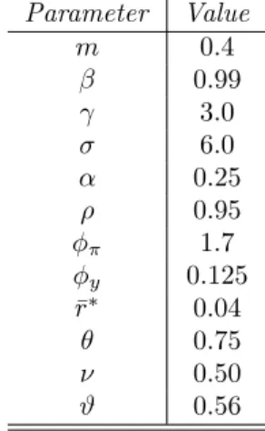
Before describing the equilibrium behavior of the prototype member economy under the framework illustrated above, we need to give a numerical value to the parameters. To this purpose we distinguish two kinds of parameters: general pa-rameters and …scal policy papa-rameters. The former(m; ; ; ; ; ; ; r ; ; ; #) are calibrated according to the benchmark parametrization adopted by Galì and Monacelli (2008) and some stylized facts about EMU countries, whereas for the latter we use the EMU data( ; ; n; k). The following table summarizes the benchmark parametrization for general parameters:

Table 1:Calibration for general parameters

Parameter Value m 0:4 0:99 3:0 6:0 0:25 0:95 1:7 y 0:125 r 0:04 0:75 0:50 # 0:56

The values calibrated for the labor supply elasticity ( ), for the elasticity of substitution between di¤erentiated goods( ), for the degree of stickiness of prices( );for the average share of public consumption( ) for EMU countries, for the subjective discount factor( ), which is in line with the real business cycle literature and implies the steady state value for interest rate(r), ensure a stable solution to the model. Moreover, following the real business cycle literature (King and Rebelo (1999)), we suppose a high value for the persistence coe¢ cient of total labor productivity( ). Finally, the index of openness with respect to EMU countries(m); the share of domestic debt held by domestic households (1 #)and the fraction of domestic …rms held by the residents(1 )are set to a value able to match statistical data about Euro-area balance of payments (source: IMF statistical data (sample 1995-2005)). Monetary policy parameters (r; )are consistent with the empirical literature about Taylor rule in the EMU (Smets and Wouters (2003)) and are in line with the Taylor principle( >1):

(20)

Table 2:Calibration for scal policy parameters Parameter Value n 0:35 k 0:24 0:85 0:51 0:20

Tax rate on labor( n)is set equal to the average annual implicit tax rate on labor employed (0.35) for the Euro area, tax rate on dividends( k)is set equal to the average implicit tax rate on capital income (0.24) for the Euro area, whereas the persistence coe¢ cient in public expenditure( ) is set equal to the average elasticity of real public expenditure with respect to its lagged value (0.85) for the Euro area (source: Eurostat statistical data (sample 1995-2005)). At the same time, we let the feedback on debt parameter ( ) assume a value equal to the average elasticity of real public expenditure with respect to lagged real stock of public debt for the Euro area (0.20) and the countercyclical parameter ( )take a value equal to the elasticity of real public expenditure with respect to output (0.51) (source: Eurostat statistical data (sample 1995-2005)). In the next section we discuss the dynamic behavior of the model both in the presence of a technology shock and of a union-wide interest rate shock under the policy rules described above.

4

Dynamic simulations under the policy rules

In this section we discuss the dynamic equilibrium behavior of a representative member economy under the model discussed above, by resorting to a series of dynamic simulations with the parameterization described in the previous section. In particular, we focus our attention on the responses of …scal policy instruments (public expenditure, tax revenues, public debt and the ratio public debt/GDP) to the domestic shock, i.e. the technology shock, and to the union-wide shock, i.e. interest rate shock.

The …rst set of …gures (Section 7.4.1.) displays the dynamic response of out-put, output gap, real public debt, the ratio debt/GDP, total private consump-tion, real public expenditure, hours worked, real wages, real marginal costs, real tax revenues and real pro…ts in the presence of a technology shock. The rigidity in aggregate demand resulting from the stickiness of the domestic price level leads technology shock (that in this framework is a labor productivity shock) to generate a negative comovement between hours worked and productivity. This result is also supported by strong empirical evidence (Galì (1999), Francis and Remy (2005); Christinano et al. (2003) among others). The intuition for this result is straightforward. When a technology shock hits the economy, the in-crease in productivity determines a fall in real marginal costs, domestic prices decrease, as a consequence of a right-shift in the aggregate supply curve and following the decrease in real marginal costs. Aggregate demand and private

(21)

consumption increase, due to the fall in domestic prices. Nevertheless, aggre-gate demand and prices, given the nominal rigidities, for which only a fraction 1 of …rms reset their prices, change less than under fully ‡exible prices. Aggregate output increases, but less than in the absence of price rigidities: for this reason, a contraction in the output gap occurs. Furthermore, because la-bor is more productive with a consequent increase in the real wages, the …rms will require less labor input. As a consequence, output does not increase in the same proportion of the productivity shock. On the other hand, real prof-its increase due both to the positive shift of output and to the contraction in real marginal costs. Real tax revenues are procyclical, i.e. with the calibra-tion adopted they increase whenever output does the same. On the contrary, public debt is countercyclical, that is, every time a positive productivity shock hits the economy and shifts upwards domestic output, government debt shows a negative deviation from its steady state value: an increase in output, leading to an increase in real tax revenues, with a countercyclical public consumption, generates a countercyclical movement of the stock of public debt. In this way, the ratio debt/GDP decreases for some periods, due to the contemporaneous contraction of the real stock of public debt and the increase in output, and then reverts to the original steady state value. Thus, public expenditure, together with taxation, plays the role of a "smoother" for output cyclical ‡uctuations.

The second set of …gures (Section 7.4.2.) displays the dynamic response of the same variables in the presence of a positive shock on the nominal interest rate. An increase in the union-wide interest rate determines a reduction in the rate of in‡ation and so in the level of prices (union-wide prices and domestic prices). The decrease in the price consumer index pushes up real wages and, at the same time, real marginal costs, that, with an invariant level of output and productivity, cause a contraction in labor demand and hence in hours worked. The reduction in labor input generates, as a consequence, a fall in output, in pro…ts and in real tax revenues. Private consumption and output decrease less than under fully ‡exible prices due to the stickiness in prices; for this reason and because of the increase in real marginal cost, an increase in the output gap occurs. Real public debt con…rms its countercyclicality as in the case of technology shock, i.e. in this case it goes up when output falls. Indeed, in this context the upper pressure of real public is strongly determined by the increase in the interest rate. In this case, the ratio debt/GDP increases for some periods, due to an expansion of the real stock of public debt and to a contraction in output, and then reverts to the original steady state value.

Hence, also in the presence of a union-wide monetary policy shock …scal pol-icy is able to stabilize output cyclical ‡uctuations through a procyclical taxation and a countercyclical public expenditure.

5

A Welfare Analysis

This section aims to evaluate …scal and monetary rules’ performances, basing on a welfare-criterion referred to country i and relying on a second-order

(22)

ap-proximation to the utility losses of the consumers. In order to measure these utility losses, we make use of a welfare function de…ned here as the discounted sum of the utilities across households:

z 1 X t=0 t_{U C}i t; Nti; Git (67) The benchmark values against which we measure the welfare losses associ-ated to our policy rules are referred to an economic framework without dis-tortionary taxation, with zero stock of public debt, with lump-sum taxation able to …nance public consumption at its optimal level and without monetary rules. In such an environment, output gap is measured as the di¤erence be-tween actual output and the fully ‡exible price one, with the latter also optimal from the social planner’s point of view, due to the absence of distortionary tax-ation. For this purpose12_{, we have to impose for each variable a steady state}

value corresponding to the one deriving from the solution of the Social Planner’s problem13.

As already shown in Galì and Monacelli (2008) a second order approximation to (67) can be rewritten as the average utility losses of union households resulting from ‡uctuations about the e¢ cient steady state in the following functional form14_: '1₂ 1 X t=0 t i t 2 + (1 + ) ~yti 2 + 1 f~ i t 2 +tips (68)

wheretipsdenotes terms that are independent of policy andf~i

t= gti yti log de…ned as …scal gap. In words, this variable represents the share of output used for public consumption less the amount of public expenditure to which the households give a weight in the utility function (log ) and for this reason it represents an ine¢ cient gap.

Taking the expected value on both side of (68) at time 0 obtains the average welfare loss per period given by the following linear combination of output gap and in‡ation variances and the variance of …scal gap:

L=1 2 var i t + (1 + )var y~ti + 1 var ~ f_ti (69) Using (69), given the monetary and …scal rules together with a calibration for the model’s parameters above described, it’s possible to compute the second order moments of the simulated time series15 _{for output gap, in‡ation and …scal}

gap, in order to derive the corresponding welfare losses associated to these rules.

1 2_{For this point we thank in particular Pierpaolo Benigno for his important suggestions.} 1 3_{These values, calculated by Galì and Monacelli (2008), are reported in Appendix.} 1 4_{For the analytical derivation of the welfare function, see Appendix in Galì and Monacelli} (2008).

(23)

Table 3 reports the measures of domestic in‡ation, output gap and …scal gap variance together with the per cent contributions to welfare losses in round brackets: in column "A" we analyse the e¤ects of the only presence of Taylor rule (26) with lump-sum taxation able to …nance public consumption at its optimal level and zero public debt, in column "B" we show the e¤ects of …scal rules (45 and 46) with no rules for monetary policy, whereas column "C" evaluates the joint e¤ects of the monetary and …scal rules.

Table 3:Contributions to Welfare Losses

Taylor Rule(A) Fiscal Rules(B) Taylor Rule+Fiscal Rules(C)

1 2 var i t 0:18 (28:57%) 0:87 (91:58%) 0:01 (25%) 1 2(1 + )var y~ i t 0:20 (31:75%) 0:05 (5:26%) 0:02 (50%) 1 2var f~ti 0:25 (39:68%) 0:03 (3:16%) 0:01 (25%) T otal 0:63 0:95 0:04

From a …rst inspection of the table, it’s evident how the mix of …scal and monetary rules (Column C) reduces welfare losses more than the single rules and so it should be preferred. The comparison between …scal rules and mone-tary rule shows that …scal rules generate larger welfare losses than Taylor rule. Furthermore from an analysis of Column A and B it emerges that Taylor rule is able to better reduce the ‡uctuations in domestic in‡ation in comparison with …scal rules, whereas both output gap and …scal gap show smaller variations in the presence of …scal rules than under Taylor rule. Finally, under the monetary rule, …scal gap has the most important role in explaining welfare losses whereas under …scal rules, this role belongs to domestic in‡ation.

From this picture two key results emerge: 1) the combination of a monetary policy, that positively responds to in‡ation and output gap, and …scal rules made up of distortionary taxation on labor, dividends and interests on public bonds and of a countercyclical and debt-stabilizing public consumption is wel-fare improving than the same …scal and monetary rules singly considered; 2) in the presence of our monetary rule domestic in‡ation variance falls more than in the presence of …scal rules, whereas output and …scal gap ‡uctuations are better smoothed by our …scal rules on public expenditure and taxation. Therefore, in a currency union scenario like the EMU, the common monetary policy should mainly focus on in‡ation stabilization, whereas …scal policy, institutionally de-centralized at a country level, should centre on output gap stabilization. This last objective can be reached in the presence of …scal rules focused not only on business cycle stabilization but also on debt stabilization, consistently with the SGP.

These …ndings have some similarities with those of Ferrero (2005). He …nds that, in the presence of a monetary rule that positively reacts to in‡ation and output gap and with a …scal constraint on real debt such that it positively reacts to output gap, such …scal policy leads to welfare gains if compared to

(24)

balanced budget rules, whereas monetary policy better smoothes in‡ation and hence should focus on price stability.

6

Conclusions

This paper develops a New-Keynesian multicountry model applied to the EMU context with sticky prices and the presence of policy rules related to …scal pol-icy and monetary polpol-icy. The former is managed by the governement sector, institutionally decentralized at a single country level, that makes use of distor-tionary taxation on labor, on dividends and interests on public bonds and of public consumption following a countercyclical and debt-stabilizing behavior. The latter is under the control of the common monetary authority, that follows a Taylor rule increased by a stochastic component driven by a monetary shock. From a welfare analysis of the policy rules we have the chance to evaluate the welfare contribution, in terms of welfare losses, of the monetary rule in a scenario without public debt and with lump-sum taxation able to …nance public consumption at its optimal level, of the …scal rules in a context without any monetary rules and of the combination of …scal rules and monetary rules.

The results obtained show that i) in the presence of our monetary rule alone, domestic in‡ation ‡uctuations are better smoothed than in the presence of our …scal rules; ii) output gap variance is smaller in the presence of …scal rules alone than whenever only the monetary rule is present; iii) the …scal-monetary policy mix made up of our rules is able to lower welfare losses more than the monetary and …scal rules in isolation.

The policy implications of these results are that i) in a currency union, like the EMU, monetary policy should have the objective of in‡ation stabilization, as institutionally indicated in the Maastricht Treaty; ii) …scal policy should centre on output gap stabilization. This aim can be pursued in the presence of …scal rules not only oriented to business cycle stabilization, that is one of the purposes assigned to …scal policy by the theory of public …nance (Musgrave (1959)), but also to debt stabilization, as prescripted by the SGP.

The theoretical structure described above calls for further analysis on several points. The model ignores capital accumulation and stickiness is only con…ned to prices and not to wages. Furthermore, it could be useful to make a distinction in the government expenditure rule between current public expenditure and capital public expenditure, in order to de…ne di¤erent behaviors of these components.

(25)

References

[1] Beetsma, R. and Jensen, H. (2005): "Monetary and Fiscal Policy in-teractions in a Micro-founded Model of a Monetary Union", Journal of international Economics, 67(2), 320-52.

[2] Benigno, P. and Woodford M. (2005): “In‡ation Stabilization and Welfare: The Case of a Distorted Steady State”, Journal of the European Economics Association 3, 1185-1236.

[3] Bullard, J. and Mitra, K. (2001): "Learning About Monetary Policy Rules", Journal of Monetary Economics, September 2002. 49(6), 1105-1129. [4] Buti, M., Franco, D. and Ongera, H. (1997): "Budgetary Policies During Recessions –Retrospective Application of the ’Stability and Growth’Pact to the Postwar Period," European Commission Economic Papers no. 121 (May).

[5] Calvo, G. (1983): "Staggered Prices in a Utility Maximizing Framework", Journal of Monetary Economics, 12, 383-398.

[6] Christiano, L., Eichenbaum, M. and Vigfusson, R. (2003): "What Happens After a Technology Shock?", NBER, Working Paper, 9819

[7] Colciago, A., Ropele, T., Muscatelli, V.A., Tirelli, P. (2008): "The Role of Fiscal Policy in a Monetary Union: are National Automatic Stabilizers E¤ective? ," Review of International Economics, Blackwell Publishing, vol. 16(3), 591-610.

[8] Ferrero, A. (2005): "Fiscal and monetary rules for a currency union," Work-ing Paper Series 502, European Central Bank.

[9] Francis, N. and Ramey, V. (2005): "Is the Technology-Driven Real Business Cycle Hypothesis Dead? Shocks and Aggregate Fluctuations Revisited", Journal of Monetary Economics, 52, 1379-1399

[10] Galì, J. and Monacelli, T. (2008): "Optimal Monetary and Fiscal Policy in a Currency Union", Economics Working Papers 909, Department of Economics and Business, Universitat Pompeu Fabra, revised Feb 2008. [11] Galì, J. and Perotti, T. (2003): "Fiscal Policy and Monetary integration in

Europe", Economic Policy, 2003, 18(37), 533-572.

[12] Galì, J. (1999): “Technology, Employment and the Business Cycle: Do Technology Shocks Explain Aggregate Fluctuations?”American Economic Review, March, 249–271.

[13] Galì, J. (2008): "Monetary Policy, in‡ation, and the Business Cycle", Princeton University Press.

(26)

[14] King, R. and Rebelo S., (1999), "Resuscitating Real Business Cycles", in J.B.Taylor, and M. Woodford, eds., Handbook of Macroeconomics, Ams-terdam: North-Holland.

[15] Melitz, J. (2000): "Some Cross-Country Evidence about Fiscal Policy Be-havior and Consequences for EMU", mimeo University of Strathclyde. [16] Muscatelli, A., Tirelli, P. and Trecroci, C. (2004): “Fiscal and monetary

policy interactions: Empirical evidence and optimal policy using a struc-tural New-Keynesian model,” Journal of Macroeconomics, 26, 257-280. [17] Musgrave R.A. (1959), The Theory of Public Finance, 1^ed., McGraw Hill,

New York.

[18] Rotemberg, J. J. and Woodford, M. (1999): "Interest Rate Rules in an Estimated Sticky Price Model", in J. B. Taylor (ed.), Monetary Policy Rules, University of Chicago Press, Chicago, IL.

[19] Schmitt-Grohe, S., and M. Uribe (2007): “Optimal Simple and imple-mentable Monetary and Fiscal Rules,” Journal of Monetary Economics, 54(6), 1702-1725.

[20] Smets, F. and Wouters R. (2003): "An Estimated Dynamic Stochastic General Equilibrium Model of the Euro Area," Journal of the European Economic Association, MiT Press, vol. 1(5), pages 1123-1175

[21] Trionfetti F. (2000), "Discriminatory Public Procurement and international Trade", Blackwell Publishers.

[22] Wyplosz, C.(2002): "Fiscal discipline in EMU: rules or institutions?", mimeo, Graduate institute for international Studies, Geneva.

(27)

7

Appendix

7.1

Pro…t maximization problem in steady state

M ax Yi₍_j₎ " Yi₍_j₎ 1 _Pi Yi 1 Wi AiY i₍_j₎ # @ i₍_j₎ @Yi₍_j₎ = 0 : 1 Yi(j) 1 Pi Yi 1 _Wi Ai = 0 1 Yi(j) 1 Pi Yi 1 _Wi Ai = 0 1 Yi(j) 1 Pi Yi 1 =W i Ai Yi₍_j₎ Yi ! 1 Pi 1 =W i Ai Pi(j) 1 = W i Ai Pi(j) = W i Ai ₁ Z 1 0 Pi(j)1 dj 1 1 = Z 1 0 Wi Ai ₁ 1 dj ! 1 1 Pi= W i Ai ₁ (70) Wi Ai_Pi = 1 =M Ci (71)

The expressiom (70) states that, in steady state, the level of pricePi given by the product of marginal costs W_Aii and markup ₁ :

7.2

Taylor expansion of

log (

Y

i t

G

it

)

Let{i= G_Y the steady state government spending share. De…ney^ti= log Yti Y and ^ git = log Gi t

G: A …rst-order Taylor expansion of log Y i

t Git about the steady state yields: log Y_ti Gi_t = log (1 {i)Y + 1 1 {i Yi t Y Y {i 1 {i Gi t G G log Y_ti Gi_t = log (1 {i)Y + 1 1 {i ^ yi_t {i^git

(28)

7.3

The e¢ cient steady-state derived by the solution of

Central Planner’s problem

The symmetric steady state implied by the solution of the Social Planner’s problem is the same as the one of Galì and Monacelli (2008). In this context taxation takes the only form of lump-sum taxes and public debt is absent:

Ni = 1 (72) Yi =Ai (73) C_ii = (1 ) (1 m)Ai (74) C_if = (1 )mAi (75) Gi = Ai (76) Ci = (1 ) Ai 1 m A m (77) Y =A (78) C = (1 ) A (79) G = A (80)

The previous conditions are supported as a fully ‡exible prices equilibrium at a decentralized level with the subsidy being equal to 1, that is the value able to completely o¤set the market distortions deriving by the monopolistic competition. Moreover, the e¢ cient allocations of the terms of trade is given by: Pi c Pi m = C i C 1 1 m = A i A

All these conditions with the time subscript represent the Social Planner’s dynamic equilibrium used as a benchmark to evaluate the policy rules.

(29)

7.4

Figures

7.4.1 Impulse response functions to a shock in technology

-5 0 5 10 15 20 25 30 35 -0.05 0 0.05 0.1 0.15 0.2

Impulse responses to a shock in technolog y

Years after shock

Per c e nt de v iati on fr om s tea dy s ta te totalconsumption -5 0 5 10 15 20 25 30 35 -0.25 -0.2 -0.15 -0.1 -0.05 0 0.05 0.1

Years after shock

Per c e nt de v iati on fr om s tea dy s ta te domesticprice

(30)

-5 0 5 10 15 20 25 30 35 -0.9 -0.8 -0.7 -0.6 -0.5 -0.4 -0.3 -0.2 -0.1 0

Impulse responses to a shock in technology

Years after shock

Per c ent d ev iat ion fr om s te ady s tat e publicdebt -5 0 5 10 15 20 25 30 35 -0.5 -0.45 -0.4 -0.35 -0.3 -0.25 -0.2 -0.15 -0.1 -0.05 0

Years after shock

Per c ent d ev iati on f rom s te ady s tat e hoursworked

(31)

-5 0 5 10 15 20 25 30 35 0 0.1 0.2 0.3 0.4 0.5 0.6 0.7 0.8 0.9

Years after shock

P er c ent dev iat ion f rom s teady s tat e output -5 0 5 10 15 20 25 30 35 -0.08 -0.07 -0.06 -0.05 -0.04 -0.03 -0.02 -0.01 0 0.01 0.02

Years after shock

Per c e nt de v iati on fr om s tea dy s ta te domestic output g ap

(32)

-5 0 5 10 15 20 25 30 35 0 0.5 1 1.5 2 2.5

Years after shock

Per c ent d ev iati on f rom s te ady s tat e realprofits -5 0 5 10 15 20 25 30 35 -6 -5 -4 -3 -2 -1 0

Years after shock

Per c ent d ev iati on fr om s te ady s tat e debt/GDP

(33)

-5 0 5 10 15 20 25 30 35 -1.4 -1.2 -1 -0.8 -0.6 -0.4 -0.2 0 0.2 0.4

Years after shock

Per c e nt d ev iati on fr om s te ad y s tat e realmarg inalcost -5 0 5 10 15 20 25 30 35 0 0.1 0.2 0.3 0.4 0.5 0.6 0.7

Years after shock

Per c e nt d ev iati on fr om s tea dy s tat e realwag es

(34)

-5 0 5 10 15 20 25 30 35 -0.6 -0.5 -0.4 -0.3 -0.2 -0.1 0 0.1

Years after shock

P er c en t d ev iati on fr om s te ad y s tate publicexpenditure -5 0 5 10 15 20 25 30 35 -0.05 0 0.05 0.1 0.15 0.2 0.25 0.3 0.35

Years after shock

Per c ent d ev iati on f rom s te ady s tat e realtaxrevenues

(35)

7.4.2 Impulse response functions to a shock in Taylor rule -5 0 5 10 15 20 25 30 35 -0.2 -0.15 -0.1 -0.05 0 0.05 0.1 0.15

Impulse responses to a shock in taylor rule

Years after shock

Per c e nt de v iati on fr om s tea dy s ta te totalconsumption -5 0 5 10 15 20 25 30 35 -0.09 -0.08 -0.07 -0.06 -0.05 -0.04 -0.03 -0.02 -0.01 0 0.01

Years after shock

Per c e nt de v iati on fr om s tea dy s ta te domesticprice

(36)

-5 0 5 10 15 20 25 30 35 -0.05 0 0.05 0.1 0.15 0.2

Years after shock

Per c e nt de v iati on fr om s tea dy s ta te publicdebt -5 0 5 10 15 20 25 30 35 -0.2 -0.15 -0.1 -0.05 0 0.05

Years after shock

Per c ent d ev iati on f rom s te ady s tat e hoursworked

(37)

-5 0 5 10 15 20 25 30 35 -0.25 -0.2 -0.15 -0.1 -0.05 0 0.05 0.1

Years after shock

Per c e nt de v iati on fr om s tea dy s ta te output -5 0 5 10 15 20 25 30 35 -0.2 0 0.2 0.4 0.6 0.8 1 1.2

Years after shock

Per c e nt d ev iati on fr om s te ad y s tat e domestic output g ap

(38)

-5 0 5 10 15 20 25 30 35 -0.6 -0.5 -0.4 -0.3 -0.2 -0.1 0 0.1

Years after shock

Per c ent d ev iat ion fr om s te ady s tat e realprofits -5 0 5 10 15 20 25 30 35 -0.1 0 0.1 0.2 0.3 0.4 0.5 0.6

Years after shock

Per c en t dev iat ion fr om s te a dy s tat e debt/GDP

(39)

-5 0 5 10 15 20 25 30 35 -0.2 0 0.2 0.4 0.6 0.8 1 1.2 1.4

Years after shock

Per c ent d ev iat ion fr om s te ady s tat e realmarginalcost -5 0 5 10 15 20 25 30 35 -0.2 0 0.2 0.4 0.6 0.8 1 1.2 1.4

Years after shock

Per c ent d ev iat ion fr om s te ady s tat e realwages

(40)

-5 0 5 10 15 20 25 30 35 -0.01 0 0.01 0.02 0.03 0.04 0.05 0.06 0.07 0.08 0.09

Years after shock

Per c ent d ev iati on f rom s te ady s tat e publicexpenditure -5 0 5 10 15 20 25 30 35 -0.09 -0.08 -0.07 -0.06 -0.05 -0.04 -0.03 -0.02 -0.01 0 0.01

Years after shock

Per c ent d ev iati on f rom s te ady s tat e realtaxrevenues