General rights
Copyright and moral rights for the publications made accessible in the public portal are retained by the authors and/or other copyright owners and it is a condition of accessing publications that users recognise and abide by the legal requirements associated with these rights.
• Users may download and print one copy of any publication from the public portal for the purpose of private study or research. • You may not further distribute the material or use it for any profit-making activity or commercial gain
• You may freely distribute the URL identifying the publication in the public portal
If you believe that this document breaches copyright please contact us providing details, and we will remove access to the work immediately and investigate your claim.
Semi-Supervised Generation with Cluster-aware Generative Models
Maaløe, Lars; Fraccaro, Marco; Winther, Ole Published in:
arXiv
Publication date: 2017
Document Version
Publisher's PDF, also known as Version of record
Link back to DTU Orbit
Citation (APA):
Maaløe, L., Fraccaro, M., & Winther, O. (2017). Semi-Supervised Generation with Cluster-aware Generative Models. arXiv.
Lars Maaløe1 Marco Fraccaro1 Ole Winther1
Abstract
Deep generative models trained with large amounts of unlabelled data have proven to be powerful within the domain of unsupervised learning. Many real life data sets contain a small amount of labelled data points, that are typi-cally disregarded when training generative mod-els. We propose the Cluster-aware Generative Model, that uses unlabelled information to in-fer a latent representation that models the natu-ral clustering of the data, and additional labelled data points to refine this clustering. The gen-erative performances of the model significantly improve when labelled information is exploited, obtaining a log-likelihood of−79.38nats on per-mutation invariant MNIST, while also achieving competitive semi-supervised classification accu-racies. The model can also be trained fully un-supervised, and still improve the log-likelihood performance with respect to related methods.
1. Introduction
Variational Auto-Encoders (VAE) (Kingma, 2013; Rezende et al., 2014) and Generative Adversarial Net-works (GAN) (Goodfellow et al., 2014) have shown promising generative performances on data from complex high-dimensional distributions. Both approaches have spawn numerous related deep generative models, not only to model data points like those in a large unlabelled training data set, but also for semi-supervised classification (Kingma et al., 2014; Maaløe et al., 2016; Springenberg, 2015; Salimans et al., 2016). In semi-supervised classifi-cation a few points in the training data are endowed with class labels, and the plethora of unlabelled data aids to improve a supervised classification model.
Could a few labelled training data points in turn improve a deep generative model? This reverse perspective, doing semi-supervised generation, is investigated in this work.
1
Technical University of Denmark. Correspondence to: Lars Maaløe<[email protected]>, Marco Fraccaro<[email protected]>, Ole Winther<[email protected]>.
Many of the real life data sets contain a small amount of labelled data, but incorporating this partial knowledge in the generative models is not straightforward, because of the risk of overfitting towards the labelled data. This over-fitting can be avoided by finding a good scheme for up-dating the parameters, like the one introduced in the mod-els for semi-supervised classification (Kingma et al., 2014; Maaløe et al., 2016). However, there is a difference in opti-mizing the model towards optimal classification accuracy and generative performance. We introduce the Cluster-aware Generative Model (CaGeM), an extension of a VAE, that improves the generative performances, by being able to model the natural clustering in the higher feature repre-sentations through a discrete variable (Bengio et al., 2013). The model can be trained fully unsupervised, but its per-formances can be further improved using labelled class in-formation that helps in constructing well defined clusters. A generative model with added labelled data information may be seen as parallel to how humans rely on abstract do-main knowledge in order to efficiently infer a causal model from property induction with very few labelled observa-tions (Tenenbaum et al., 2006).
Supervised deep learning models with no stochastic units are able to learn multiple levels of feature abstraction. In VAEs, however, the addition of more stochastic layers is often accompanied with a built-in pruning effect so that the higher layers become disconnected and therefore not ex-ploited by the model (Burda et al., 2015a; Sønderby et al., 2016). As we will see, in CaGeM the possibility of learn-ing a representation in the higher stochastic layers that can model clusters in the data drastically reduces this issue. This results in a model that is able to disentangle some of the factors of variation in the data and that extracts a hierarchy of features beneficial during the generation phase. By using only 100 labelled data points, we present state of the art log-likelihood performance on permutation-invariant models for MNIST, and an improvement with re-spect to comparable models on the OMNIGLOT data set. While the main focus of this paper is semi-supervised gen-eration, we also show that the same model is able to achieve competitive semi-supervised classification results.
2. Variational Auto-encoders
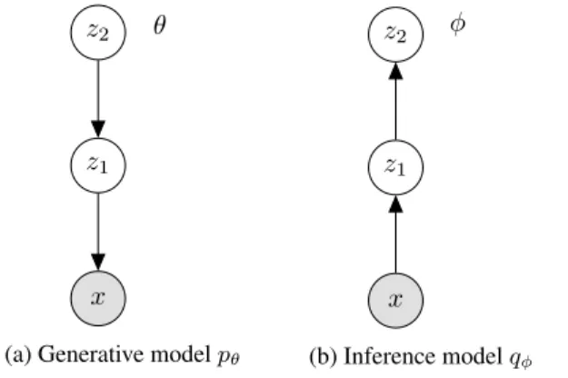
A Variational Auto-Encoder (VAE) (Kingma, 2013; Rezende et al., 2014) defines a deep generative model for dataxthat depends on latent variablezor a hierarchy of latent variables, e.g.z= [z1, z2], see Figure 1a for a
graph-ical representation. The joint distribution of the two-level generative model is given by
pθ(x, z1, z2) =pθ(x|z1)pθ(z1|z2)p(z2),
where
pθ(z1|z2) =N(z1;µ1θ(z2), σ1θ(z2))
p(z2) =N(z2; 0, I)
are Gaussian distributions with a diagonal covariance ma-trix and pθ(x|z1) is typically a parameterized Gaussian
(continuous data) or Bernoulli distribution (binary data). The probability distributions of the generative model of a VAE are parameterized using deep neural networks whose parameters are denoted byθ. Training is performed by opti-mizing theEvidence Lower Bound (ELBO), a lower bound to the intractable log-likelihood logpθ(x) obtained using Jensen’s inequality: logpθ(x) = log Z Z pθ(x, z1, z2)dz1dz2 ≥Eqφ(z1,z2|x) logpθ(x, z1, z2) qφ(z1, z2|x) =F(θ, φ). (1) The introduced variational distribution qφ(z1, z2|x) is
an approximation to the model’s posterior distribution
pθ(z1, z2|x), defined with a bottom-up dependency
struc-ture where each variable of the model depends on the vari-able below in the hierarchy:
qφ(z1, z2|x) =qφ(z1|x)qφ(z2|z1)
qφ(z1|x) =N(z1;µ1φ(x), σ
1
φ(x))
qφ(z2|z1) =N(z2;µ2φ(z1), σ2φ(z1)).
Similar to the generative model, the mean and diagonal co-variance of both Gaussian distributions defining the infer-ence network qφ are parameterized with deep neural net-works that depend on parameters φ, see Figure 1b for a graphical representation.
We can learn the parametersθandφby jointly maximiz-ing the ELBOF(θ, φ)in (1) with stochastic gradient as-cent, using Monte Carlo integration to approximate the intractable expectations and computing low variance gra-dients with the reparameterization trick (Kingma, 2013; Rezende et al., 2014).
x z1
z2 θ
(a) Generative modelpθ
x z1
z2 φ
(b) Inference modelqφ Figure 1: Generative model and inference model of a Vari-ational Auto-Encoder with two stochastic layers.
Inactive stochastic units A common problem encoun-tered when training VAEs with bottom-up inference net-works is given by the so called inactive units in the higher layers of stochastic variables (Burda et al., 2015a; Sønderby et al., 2016). In a 2-layer model for example, VAEs often learnqφ(z2|z1) =p(z2) =N(z2; 0, I), i.e. the
variational approximation ofz2uses no information
com-ing from the data point x through z1. If we rewrite the
ELBO in (1) as F(θ, φ) =Eqφ(z1,z2|x) logpθ(x, z1|z2) qφ(z1|x) − Eqφ(z1|x)[KL[qφ(z2|z1)||p(z2)]] we can see thatqφ(z2|z1) =p(z2)represents a local
max-ima of our optimization problem where the KL-divergence term is set to zero and the information flows by first sam-pling inze1 ∼qφ(z1|x)and then computingpθ(x|ze1)(and is therefore independent fromz2). Several techniques have
been developed in the literature to mitigate the problem of inactive units, among which we find annealing of the KL term (Bowman et al., 2015; Sønderby et al., 2016) or the use of free bits (Kingma et al., 2016).
Using ideas from Chen et al. (2017), we notice that the in-active units in a VAE with 2 layers of stochastic units can be justified not only as a poor local maxima, but also from the modelling point of view. Chen et al. (2017) give abits-back codinginterpretation of Variational Inference for a genera-tive model of the formp(x, z) = p(x|z)p(z), with datax
and stochastic unitsz. The paper shows that if the decoder
p(x|z)is powerful enough to explain most of the structure in the data (e.g. an autoregressive decoder), then it will be convenient for the model to setq(z|x) =p(z)not to incur in an extra optimization cost ofKL[q(z|x)||p(z|x)]. The inactivez2units in a 2-layer VAE can therefore be seen as
caused by the flexible distributionpθ(x, z1|z2)that is able
to explain most of the structure in the data without using information fromz2. By makingqφ(z2|z1) = p(z2), the
model can avoid the extra cost ofKL[qφ(z2|x)||pθ(z2|x)].
A more detailed discussion on the topic can be found in Appendix A.
It is now clear that if we want a VAE to exploit the power of additional stochastic layers we need to define it so that the benefits of encoding meaningful information inz2is greater than the costKL[qφ(z2|x)||pθ(z2|x)]that
the model has to pay. As we will discuss below, we will achieve this by aiding the generative model to do represen-tation learning.
3. Cluster-aware Generative Models
Hierarchical models parameterized by deep neural net-works have the ability to represent very flexible distribu-tions. However, in the previous section we have seen that the units in the higher stochastic layers of a VAE often be-come inactive. We will show that we can help the model to exploit the higher stochastic layers by explicitly encoding a useful representation, i.e. the ability to model the natural clustering of the data (Bengio et al., 2013), which will also be needed for semi-supervised generation.
We favor the flow of higher-level global information through z2 by extending the generative model of a VAE
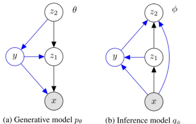
with a discrete variable y representing the choice of one out ofKdifferent clusters in the data. The joint distribu-tionpθ(x, z1, z2)is computed by marginalizing overy:
pθ(x, z1, z2) = X y pθ(x, y, z1, z2) =X y pθ(x|y, z1)pθ(z1|y, z2)pθ(y|z2)p(z2).
We call this model Cluster-aware Generative Model (CaGeM), see Figure 2 for a graphical representa-tion. The introduced categorical distributionpθ(y|z2) =
Cat(y;πθ(z2)) (πθ represents the class distribution) de-pends solely onz2, that needs therefore to stay active for
the model to be able to represent clusters in the data. We further add the dependence ofz1andxony, so that they
can now both also represent cluster-dependent information. 3.1. Inference
As done for the VAE in (1), we can derive the ELBO for CaGeM by maximizing the log-likelihood
logpθ(x) = log Z Z pθ(x, z1, z2)dz1dz2 = log Z Z X y pθ(x, y, z1, z2)dz1dz2 ≥Eqφ(y,z1,z2|x) logpθ(x, y, z1, z2) qφ(y, z1, z2|x) . x y z1 z2 θ
(a) Generative modelpθ
x
y z1
z2 φ
(b) Inference modelqφ Figure 2: Generative model and inference model of a CaGeM with two stochastic layers (black and blue lines). The black lines only represent a standard VAE.
We define the variational approximation qφ(y, z1, z2|x)
over the latent variables of the model as
qφ(y, z1, z2|x) =qφ(z2|x, y, z1)qφ(y|z1, x)qφ(z1|x), where qφ(z1|x) =N(z1;µ1φ(x), σ 1 φ(x)) qφ(z2|x, y, z1) =N(z2;µ2φ(y, z1), σ2φ(y, z1)) qφ(y|z1, x) =Cat(y;πφ(z1, x))
In the inference network we then reverse all the dependen-cies among random variables in the generative model (the arrows in the graphical model in Figure 2). This results in abottom-up inference network that performs a feature extraction that is fundamental for learning a good repre-sentation of the data. Starting from the dataxwe construct higher levels of abstraction, first through the variables z1
andy, and finally through the variablez2, that includes the
global information used in the generative model. In order to make the higher representation more expressive we add a skip-connection fromxtoz2, that is however not
funda-mental to improve the performances of the model.
With this factorization of the variational distribution
qφ(y, z1, z2|x), the ELBO can be written as
F(θ, φ) =Eqφ(z1|x) " X y qφ(y|z1, x)· ·Eqφ(z2|x,y,z1) logpθ(x, y, z1, z2) qφ(y, z1, z2|x) .
We maximizeF(θ, φ)by jointly updating, with stochastic gradient ascent, the parametersθ of the generative model andφof the variational approximation. When computing the gradients, the summation overy is performed analyti-cally, whereas the intractable expectations overz1 andz2
are approximated by sampling. We use the reparameteriza-tion trick to reduce the variance of the stochastic gradients.
4. Semi-Supervised Generation with CaGeM
In some applications we may have class label information for some of the data points in the training set. In the fol-lowing we will show that CaGeM provides a natural way to exploit additional labelled data to improve the performance of the generative model. Notice that thissemi-supervised generationapproach differs from the more traditional semi-supervised classification task that uses unlabelled data to improve classification accuracies (Kingma et al., 2014; Maaløe et al., 2016; Salimans et al., 2016). In our case in fact, it is the labelled data that supports the generative task. Nevertheless, we will see in our experiment that CaGeM also leads to competitive semi-supervised classi-fication performances.To exploit the class information, we first set the number of clustersKequal to the number of classesC. We can now define two classifiers in CaGeM:
1. In the inference network we can compute the class probabilities given the data, i.e. qφ(y|x), by integrat-ing out the stochastic variablesz1fromqφ(y, z1|x)
qφ(y|x) = Z qφ(y, z1|x)dz1 = Z qφ(y|z1, x)qφ(z1|x)dz1
2. Another set of class-probabilities can be computed us-ing the generative model. Given the posterior distribu-tionpθ(z2|x)we have in fact
pθ(y|x) = Z
pθ(y|z2)pθ(z2|x)dz2.
The posterior over z2 is intractable, but we can
approximate it using the variational approximation
qφ(z2|x), that is obtained by marginalizing outy and
the variablez1in the joint distributionqφ(y, z1, z2|x):
pθ(y|x)≈ Z pθ(y|z2)qφ(z2|x)dz2 = Z pθ(y|z2) Z X e y qφ(z2|x,y, ze 1)· ·qφ(ye|z1, x)qφ(z1|x)dz1 ! dz2.
While for the labelsyethe summation can be carried out analytically, for the variable z1 and z2 we use
Monte Carlo integration. For each of theCclasses we will then obtain a differentzc
2sample (c = 1, . . . C)
with a corresponding weight given by qφ(eyc|z1, x).
This therefore resembles a cascadeof classifiers, as the class probabilities of thepθ(y|x)classifier will de-pend on the probabilities of the classifierqφ(y|z1, x)
in the inference model.
As our main goal is to learn representations that will lead to good generative performance, we interpret the classifi-cation of the additional labelled data as a secondary task that aids in learning a z2 feature space that can be easily
separated into clusters. We can then see this as a form of semi-supervised clustering (Basu et al., 2002), where we know that some data points belong to the same cluster and we are free to learn a data manifold that makes this possi-ble.
The optimal features for the classification task could be very different from the representations learned for the gen-erative task. This is why it is important not to update the parameters of the distributions overz1,z2 andx, in both
generative model and inference model, using labelled data information. If this is not done carefully, the model could be prone to overfitting towards the labelled data. We define asθythe subset ofθcontaining the parameters inpθ(y|z2),
and as φy the subset of φ containing the parameters in
qφ(y|z1, x).θyandφythen represent the incoming arrows toyin Figure 2. We update the parametersθandφjointly by maximizing the new objective
I= X {xu} F(θ, φ)−α X {xl,yl} (Hp(θy, φy) +Hq(φy))
where{xu}is the set of unlabelled training points,{xl, yl} is the set of labelled ones, andHpandHqare the standard categorical cross-entropies for the pθ(y|x) and qφ(y|x) classifiers respectively. Notice that we consider the cross-entropies only a function of θy andφy, meaning that the gradients of the cross-entropies with respect to the param-eters of the distributions overz1,z2 andxwill be 0, and
will not depend on the labelled data (as needed when learn-ing meanlearn-ingful representations of the data to be used for the generative task). To match the relative magnitudes be-tween the ELBO F(θ, φ)and the two cross-entropies we setα=βNuN+Nl
l as done in (Kingma et al., 2014; Maaløe et al., 2016), where Nu andNl are the numbers of unla-belled and launla-belled data points, andβis a scaling constant.
5. Experiments
We evaluate CaGeM by computing the generative log-likelihood performance on MNIST and OMNIGLOT (Lake et al., 2013) datasets. The model is parameterized by feed-forward neural networks (NN) and linear layers (Linear),
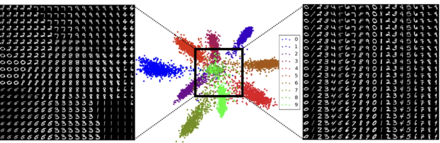
Figure 3: Visualizations from CaGeM-100 with a 2-dimensionalz2space. The middle plot shows the latent space, from
which we generate random samples (left) and class conditional random samples (right) with a mesh grid (black bounding box). The relative placement of the samples in the scatter plot corresponds to a digit in the mesh grid.
so that, for Gaussian outputs, each collection of incoming edges to a node in Figure 2 is defined as:
d=NN(x) µ=Linear(d) logσ=Linear(d).
For Bernoulli distributed outputs we simply define a feed-forward neural network with a sigmoid activation func-tion for the output. Between dense layers we use the rec-tified linear unit as non-linearity and batch-normalization (Ioffe & Szegedy, 2015). We only collect statistics for the batch-normalization during unlabelled inference. For the log-likelihood experiments we apply temperature on the
KL-terms during the first 100 epochs of training (Bow-man et al., 2015; Sønderby et al., 2016). The stochastic layers are defined withdim(z1) = 64,dim(z2) = 32and
2-layered neural feed-forward networks with respectively 1024 and 512 units in each layer. Training is performed using the Adam optimizer (Kingma & Ba, 2014) with an initial learning rate of0.001and annealing it by.75every
50epochs. The experiments are implemented with Theano (Bastien et al., 2012), Lasagne (Dieleman et al., 2015) and Parmesan1.
For both datasets we report unsupervised and semi-supervised permutation invariant log-likelihood perfor-mance and for MNIST we also report semi-supervised clas-sification errors. The input data is dynamically binarized and the ELBO is evaluated by taking 5000 importance-weighted (IW) samples, denotedF5000. We evaluate the
performance of CaGeM with different numbers of labelled samples referred to as CaGeM-#labels. When used, the labelled data is randomly sampled evenly across the class distribution. All experiments across datasets are run with the same architecture.
1A variational repository named parmesan on Github.
6. Results
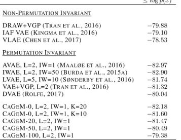
Table 1 shows the generative log-likelihood performances of different variants of CaGeM on the MNIST data set. We can see that the more labelled samples we use, the better the generative performance will be. Even though the re-sults are not directly comparable, since CaGeM exploits a small fraction supervised information, we find that using only 100 labelled samples (10 samples per class), CaGeM-100 model achieves state of the art log-likelihood perfor-mance on permutation invariant MNIST with a simple 2-layered model. We also trained a ADGM-100 from Maaløe et al. (2016)2in order to make a fair comparison on genera-tive log-likelihood in a semi-supervised setting and reached a performance of−86.06nats. This indicates that models that are highly optimized for improving semi-supervised classification accuracy may be a suboptimal choice for gen-erative modeling.
CaGeM could further benefit from the usage of non-permutation invariant architectures suited for image data, such as the autoregressive decoders used by IAF VAE (Kingma et al., 2016) and VLAE (Chen et al., 2017). The fully unsupervised CaGeM-0 results show that by defin-ing clusters in the higher stochastic units, we achieve better performances than the closely related IWAE (Burda et al., 2015a) and LVAE (Sønderby et al., 2016) models. It is fi-nally interesting to see from Table 1 that CaGeM-0 per-forms well even when the number of clusters are different from the number of classes in the labelled data set. In Figure 4 we show in detail how the performance of CaGeM increases as we add more labelled data points. We can also see that the ELBO Ftest
1 tightens when
2
We used the code supplied in the repository named auxiliary-deep-generative-models on Github.
≤logp(x)
NON-PERMUTATIONINVARIANT
DRAW+VGP (TRAN ET AL., 2016) −79.88
IAF VAE (KINGMA ET AL., 2016) −79.10
VLAE (CHEN ET AL., 2017) −78.53
PERMUTATIONINVARIANT
AVAE, L=2, IW=1 (MAALØE ET AL., 2016) −82.97
IWAE, L=2, IW=50 (BURDA ET AL., 2015A) −82.90
LVAE, L=5, IW=10 (SØNDERBY ET AL., 2016) −81.74
VAE+VGP, L=2 (TRAN ET AL., 2016) −81.32 DVAE (ROLFE, 2017) −80.04 CAGEM-0, L=2, IW=1, K=20 −82.18 CAGEM-0, L=2, IW=1, K=10 −81.60 CAGEM-20, L=2, IW=1 −81.47 CAGEM-50, L=2, IW=1 −80.49 CAGEM-100, L=2, IW=1 −79.38
Table 1: Test log-likelihood for permutation invariant and non-permutation invariant MNIST. L, IW and K denotes the number of stochastic layers (if it is translatable to the VAE), the number of importance weighted samples used during inference, and the number of predefined clusters used.
adding more labelled information, as compared toFLVAE
1 =
−85.23andFVAE
1 =−87.49(Sønderby et al., 2016).
The PCA plots of thez2variable of a VAE, CaGeM-0 and
CaGeM-100 are shown in Figure 5 . We see how CaGeMs encode clustered information into the higher stochastic layer. Since CaGeM-0 is unsupervised, it forms less class-dependent clusters compared to the semi-supervised CaGeM-100, that fits its z2 latent space into 10 nicely
separated clusters. Regardless of the labelled informa-tion added during inference, CaGeM manages to acti-vate a high amount of units, as for CaGeM we obtain
KL[qφ(z2|x, y)||p(z2)] ≈ 17nats, while a LVAE with 2
stochastic layers obtains≈9nats.
The generative model in CaGeM enables both random sam-ples, by sampling the class variabley∼pθ(y|z2)and
feed-ing it topθ(x|z1, y), and class conditional samples by
fix-ingy. Figure 3 shows the generation of MNIST digits from CaGeM-100 with dim(z2) = 2. The images are
gener-ated by applying a linearly spaced mesh grid within the la-tent spacez2and performing random generations (left) and
conditional generations (right). When generating samples in CaGeM, it is clear how the latent unitsz1 andz2
cap-ture different modalities within the true data distribution, namely style and class.
Regardless of the fact that CaGeM was designed to op-timize the semi-supervised generation task, the model can also be used for classification by using the classifier
pθ(y|x). In Table 2 we show that the semi-supervised clas-sification accuracies obtained with CaGeM are comparable
Figure 4: Log-likelihood scores for CaGeM on MNIST with 0, 20, 50 and 100 labels with 1, 10 and 5000 IW sam-ples.
Figure 5: PCA plots of the stochastic unitsz1andz2in a
2-layered model trained on MNIST. The colors corresponds to the true labels.
to the performance of GANs (Salimans et al., 2016). The OMNIGLOT dataset consists of 50 different alphabets of handwritten characters, where each character is sparsely represented. In this task we use the alphabets as the clus-ter information, so that thez2representation should divide
LABELS 20 50 100
M1+M2 (KINGMA ET AL., 2014) - - 3.33% (±0.14)
VAT (MIYATO ET AL., 2015) - - 2.12%
CATGAN (SPRINGENBERG, 2015) - - 1.91% (±0.1)
SDGM (MAALØE ET AL., 2016) - - 1.32% (±0.07)
LADDERNETWORK(RASMUS ET AL., 2015) - - 1.06% (±0.37)
ADGM (MAALØE ET AL., 2016) - - 0.96% (±0.02)
IMP. GAN (SALIMANS ET AL., 2016) 16.77% (±4.52) 2.21% (±1.36) 0.93% (±0.65)
CAGEM 15.86% 2.42% 1.16%
Table 2: Semi-supervised test error % benchmarks on MNIST for 20, 50, and 100 randomly chosen and evenly distributed labelled samples. Each experiment was run 3 times with different labelled subsets and the reported accuracy is the mean value.
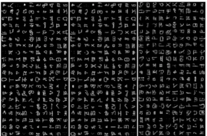
over other comparable VAE architectures (VAE, IWAE and LVAE), however, the performance is far from the once reported from the auto-regressive models (Kingma et al., 2016; Chen et al., 2017). This indicates that the alphabet in-formation is not as strong as for a dataset like MNIST. This is also indicated from the accuracy of CaGeM-500, reach-ing a performance of≈24%. Samples from the model can be found in Figure 6.
Figure 6: Generations from CaGeM-500. (left) The input images, (middle) the reconstructions, and (right) random samples fromz2.
≤logp(x)
VAE, L=2, IW=50 (BURDA ET AL., 2015A) −106.30
IWAE, L=2, IW=50 (BURDA ET AL., 2015A) −103.38
LVAE, L=5, FT, IW=10 (SØNDERBY ET AL., 2016) −102.11
RBM (BURDA ET AL., 2015B) −100.46
DBN (BURDA ET AL., 2015B) −100.45
DVAE (ROLFE, 2017) −97.43
CAGEM-500, L=2, IW=1 −100.86
Table 3: Generative test log-likelihood for permutation in-variant OMNIGLOT.
7. Discussion
As we have seen from our experiments, CaGeM offers a way to exploit the added flexibility of a second layer of
stochastic units, that stays active as the modeling perfor-mances can greatly benefit from capturing the natural clus-tering of the data. Other recent works have presented al-ternative methods to mitigate the problem of inactive units when training flexible models defined by a hierarchy of stochastic layers. Burda et al. (2015a) used importance samples to improve the tightness of the ELBO, and showed that this new training objective helped in activating the units of a 2-layer VAE. Sønderby et al. (2016) trained Lad-der Variational AutoencoLad-ders (LVAE) composed of up to 5 layers of stochastic units, using a top-down inference network that forces the information to flow in the higher stochastic layers. Contrarily to the bottom-up inference network of CaGeM, the top-down approach used in LVAEs does not enforce a clear separation between the role of each stochastic unit, as proven by the fact that all of them encode some class information. Longer hierarchies of stochastic units unrolled in time can be found in the sequential set-ting (Krishnan et al., 2015; Fraccaro et al., 2016). In these applications the problem of inactive stochastic units ap-pears when using powerful autoregressive decoders (Frac-caro et al., 2016; Chen et al., 2017), but is mitigated by the fact that new data information enters the model at each time step.
The discrete variable y of CaGeM was introduced to be able to define a better learnable representation of the data, that helps in activating the higher stochastic layer. The combination of discrete and continuous variables for deep generative models was also recently explored by several au-thors. Maddison et al. (2016); Jang et al. (2016) used a continuous relaxation of the discrete variables, that makes it possible to efficiently train the model using stochastic backpropagation. The introduced Gumbel-Softmax vari-ables allow to sacrifice log-likelihood performances to avoid the computationally expensive integration over y. Rolfe (2017) presents a new class of probabilistic models that combines an undirected component consisting of a bi-partite Boltzmann machine with binary units and a directed component with multiple layers of continuous variables.
Traditionally, semi-supervised learning applications of deep generative models such as Variational Auto-encoders and Generative Adversarial Networks (Goodfellow et al., 2014) have shown that, whenever only a small fraction of labelled data is available, the supervised classification task can benefit from additional unlabelled data (Kingma et al., 2014; Maaløe et al., 2016; Salimans et al., 2016). In this work we consider the semi-supervised problem from a different perspective, and show that the generative task of CaGeM can benefit from additional labelled data. As a by-product of our model however, we also obtain com-petitive semi-supervised classification results, meaning that CaGeM is able to share statistical strength between the gen-erative and classification tasks.
When modeling natural images, the performance of CaGeM could be further improved using more powerful au-toregressive decoders such as the ones in (Gulrajani et al., 2016; Chen et al., 2017). Also, an even more flexible vari-ational approximation could be obtained using auxiliary variables (Ranganath et al., 2015; Maaløe et al., 2016) or normalizing flows (Rezende & Mohamed, 2015; Kingma et al., 2016).
8. Conclusion
In this work we have shown how to perform semi-supervised generation with CaGeM. We showed that CaGeM improves the generative log-likelihood perfor-mance over similar deep generative approaches by creating clusters for the data in its higher latent representations us-ing unlabelled information. CaGeM also provides a natural way to refine the clusters using additional labelled informa-tion to further improve its modelling power.
A. The Problem of Inactive Units
First consider a modelp(x)without latent units. We con-sider the asymptotic average properties, so we take the ex-pectation of the log-likelihood over the (unknown) data dis-tributionpdata(x):
Epdata(x)[logp(x)] =Epdata(x)
logpdata(x) p(x) pdata(x) =−H(pdata)−KL(pdata(x)||p(x)),
whereH(p) =−Ep(x)[logp(x)]is the entropy of the
dis-tribution andKL(·||·)is the KL-divergence. The expected log-likelihood is then simply the baseline entropy of the data generating distribution minus the deviation between the data generating distribution and our model for the dis-tribution.
For the latent variable modelplat(x) =
R
p(x|z)p(z)dzthe
log-likelihood bound is:
logplat(x)≥Eq(z|x) logp(x|z)p(z) q(z|x) .
We take the expectation over the data generating distribu-tion and apply the same steps as above
Epdata(x)[logplat(x)]≥Epdata(x)Eq(z|x)
logp(x|z)p(z)
q(z|x)
=−H(pdata)−KL(pdata(x)||plat(x))
−Epdata(x)[KL(q(z|x)||p(z|x))] , where p(z|x) = p(x|z)p(z)/plat(x) is the (intractable)
posterior of the latent variable model. This results shows that we pay an additional price (the last term) for using an approximation to the posterior.
The latent variable model can choose to ignore the latent variables,p(x|z) = ˆp(x). When this happens the expres-sion falls back to the log-likelihood without latent vari-ables. We can therefore get an (intractable) condition for when it is advantageous for the model to use the latent vari-ables:
Epdata(x)[logplat(x))]>Epdata(x)[log ˆp(x))] +
Epdata(x)[KL(q(z|x)||p(z|x))] . The model will use latent variables when the log-likelihood gain is so high that it can compensate for the loss
KL(q(z|x)||plat(z|x)) we pay by using an approximate
posterior distribution.
The above argument can also be used to understand why it is harder to get additional layers of latent variables to become active. For a two-layer latent variable model
p(x, z1, z2) = p(x|z1)p(z1|z2)p(z2)we use a variational
distribution q(z1, z2|x) = q(z2|z1, x)q(z1|x) and
de-compose the log likelihood bound using p(x, z1, z2) =
p(z2|z1, x)p(z1|x)plat,2(x):
Epdata(x)[logplat,2(x)]
≥Epdata(x)Eq(z1,z2|x)
logp(x|z1)p(z1|z2)p(z2)
q(z1, z2|x)
=−H(pdata)−KL(pdata(x)||plat,2(x))
−Epdata(x)Eq(z1|x)[KL(q(z2|z1, x)||p(z2|z1, x))]
−Epdata(x)KL(q(z1|x)||p(z1|x)).
Again this expression falls back to the one-layer model whenp(z1|z2) = ˆp(z1). So whether to use the second layer
of stochastic units will depend upon the potential diminish-ing return in terms of log likelihood relative to the extra
Acknowledgements
We thank Ulrich Paquet for fruitful feedback. The re-search was supported by Danish Innovation Foundation, the NVIDIA Corporation with the donation of TITAN X GPUs. Marco Fraccaro is supported by Microsoft Research through its PhD Scholarship Programme.
References
Bastien, Fr´ed´eric, Lamblin, Pascal, Pascanu, Razvan, Bergstra, James, Goodfellow, Ian J., Bergeron, Arnaud, Bouchard, Nicolas, and Bengio, Yoshua. Theano: new features and speed improvements. InDeep Learning and Unsupervised Feature Learning, workshop at Neural In-formation Processing Systems, 2012.
Basu, Sugato, Banerjee, Arindam, and Mooney, Ray-mond J. Semi-supervised clustering by seeding. In Proceedings of the International Conference on Machine Learning, 2002.
Bengio, Yoshua, Courville, Aaron, and Vincent, Pascal. Representation learning: A review and new perspectives. IEEE Transactions on Pattern Analysis and Machine In-telligence, 35(8), 2013.
Bowman, S.R., Vilnis, L., Vinyals, O., Dai, A.M., Joze-fowicz, R., and Bengio, S. Generating sentences from a continuous space. arXiv preprint arXiv:1511.06349, 2015.
Burda, Yuri, Grosse, Roger, and Salakhutdinov, Ruslan. Importance Weighted Autoencoders. arXiv preprint arXiv:1509.00519, 2015a.
Burda, Yuri, Grosse, Roger, and Salakhutdinov, Rus-lan. Accurate and conservative estimates of mrf log-likelihood using reverse annealing. InProceedings of the International Conference on Artificial Intelligence and Statistics, 2015b.
Chen, Xi, Kingma, Diederik P., Salimans, Tim, Duan, Yan, Dhariwal, Prafulla, Schulman, John, Sutskever, Ilya, and Abbeel, Pieter. Variational Lossy Autoencoder. In Inter-national Conference on Learning Representations, 2017. Dieleman, Sander, Schlter, Jan, Raffel, Colin, Olson, Eben, Sønderby, Søren K, Nouri, Daniel, van den Oord, Aaron, and and, Eric Battenberg. Lasagne: First release., Au-gust 2015.
Fraccaro, Marco, Sønderby, Søren Kaae, Paquet, Ul-rich, and Winther, Ole. Sequential neural models with stochastic layers. In Advances in Neural Information Processing Systems. 2016.
Goodfellow, Ian, Pouget-Abadie, Jean, Mirza, Mehdi, Xu, Bing, Warde-Farley, David, Ozair, Sherjil, Courville, Aaron, and Bengio, Yoshua. Generative adversarial nets. InAdvances in Neural Information Processing Systems. 2014.
Gulrajani, Ishaan, Kumar, Kundan, Ahmed, Faruk, Ali Taiga, Adrien, Visin, Francesco, Vazquez, David, and Courville, Aaron. PixelVAE: A latent variable model for natural images.arXiv e-prints, 1611.05013, Novem-ber 2016.
Ioffe, Sergey and Szegedy, Christian. Batch normalization: Accelerating deep network training by reducing internal covariate shift. InProceedings of International Confer-ence on Machine Learning, 2015.
Jang, Eric, Gu, Shixiang, and Poole, Ben. Categorical reparameterization with gumbel-softmax.arXiv preprint arXiv:1611.01144, 2016.
Kingma, Diederik and Ba, Jimmy. Adam: A Method for Stochastic Optimization. arXiv preprint arXiv:1412.6980, 12 2014.
Kingma, Diederik P., Rezende, Danilo Jimenez, Mohamed, Shakir, and Welling, Max. Semi-Supervised Learning with Deep Generative Models. In Proceedings of the International Conference on Machine Learning, 2014. Kingma, Diederik P, Salimans, Tim, Jozefowicz, Rafal,
Chen, Xi, Sutskever, Ilya, and Welling, Max. Improved variational inference with inverse autoregressive flow. InAdvances in Neural Information Processing Systems. 2016.
Kingma, Diederik P; Welling, Max. Auto-Encoding Varia-tional Bayes. arXiv preprint arXiv:1312.6114, 12 2013. Krishnan, Rahul G, Shalit, Uri, and Sontag, David. Deep
Kalman filters.arXiv:1511.05121, 2015.
Lake, Brenden M, Salakhutdinov, Ruslan R, and Tenen-baum, Josh. One-shot learning by inverting a composi-tional causal process. InAdvances in Neural Information Processing Systems. 2013.
Maaløe, Lars, Sønderby, Casper K., Sønderby, Søren K., and Winther, Ole. Auxiliary Deep Generative Models. In Proceedings of the International Conference on Machine Learning, 2016.
Maddison, Chris J., Mnih, Andriy, and Teh, Yee Whye. The concrete distribution: A continuous relax-ation of discrete random variables. arXiv preprint arXiv:1611.00712, abs/1611.00712, 2016.
Miyato, Takeru, Maeda, Shin-ichi, Koyama, Masanori, Nakae, Ken, and Ishii, Shin. Distributional Smooth-ing with Virtual Adversarial TrainSmooth-ing. arXiv preprint arXiv:1507.00677, 7 2015.
Ranganath, Rajesh, Tran, Dustin, and Blei, David M. Hierarchical variational models. arXiv preprint arXiv:1511.02386, 11 2015.
Rasmus, Antti, Berglund, Mathias, Honkala, Mikko, Valpola, Harri, and Raiko, Tapani. Semi-supervised learning with ladder networks. InAdvances in Neural Information Processing Systems, 2015.
Rezende, Danilo J., Mohamed, Shakir, and Wierstra, Daan. Stochastic Backpropagation and Approximate Inference in Deep Generative Models. arXiv preprint arXiv:1401.4082, 04 2014.
Rezende, Danilo Jimenez and Mohamed, Shakir. Varia-tional Inference with Normalizing Flows. In Proceed-ings of the International Conference on Machine Learn-ing, 2015.
Rolfe, Jason Tyler. Discrete variational autoencoders. In Proceedings of the International Conference on Learn-ing Representations, 2017.
Salimans, T., Goodfellow, I., Zaremba, W., Cheung, V., Radford, A., and Chen, X. Improved techniques for training gans. arXiv preprint arXiv:1606.03498, 2016. Sønderby, Casper Kaae, Raiko, Tapani, Maaløe, Lars,
Sønderby, Søren Kaae, and Winther, Ole. Ladder varia-tional autoencoders. InAdvances in Neural Information Processing Systems 29. 2016.
Springenberg, J.T. Unsupervised and semi-supervised learning with categorical generative adversarial net-works. arXiv preprint arXiv:1511.06390, 2015.
Tenenbaum, Joshua B., Griffiths, Thomas L., and Kemp, Charles. Theory-based Bayesian models of inductive learning and reasoning. Trends in cognitive sciences, 10 (7):309–318, July 2006.
Tran, Dustin, Ranganath, Rajesh, and Blei, David M. Vari-ational Gaussian process. InProceedings of the Interna-tional Conference on Learning Representations, 2016.