Bayesian grouped variable selection

(1)

Bayesian Grouped Variable Selection

Inauguraldissertation

zur

Erlangung der W¨urde eines Doktors der Philosophie vorgelegt der

Philosophisch-Naturwissenschaftlichen Fakult¨at der Universit¨at Basel

von

Sudhir Shankar Raman

aus Chennai,Indien

Basel, 2012

Original document stored on the publication server of the University of Basel edoc.unibas.ch

This work is licenced under the agreement „Attribution Non-Commercial No Derivatives – 2.5 Switzerland“. The complete text may be viewed here: creativecommons.org/licenses/by-nc-nd/2.5/ch/deed.en

(2)

You are free:

to Share — to copy, distribute and transmit the work

Under the following conditions:

Attribution. You must attribute the work in the manner specified by the author or licensor (but not in any way that suggests that they endorse you or your use of the work).

Noncommercial. You may not use this work for commercial purposes.

No Derivative Works. You may not alter, transform, or build upon this work.

• For any reuse or distribution, you must make clear to others the license terms of this work. The best way to do this is with a link to this web page.

• Any of the above conditions can be waived if you get permission from the copyright holder. • Nothing in this license impairs or restricts the author's moral rights.

Your fair dealing and other rights are in no way affected by the above.

This is a human-readable summary of the Legal Code (the full license) available in German:

http://creativecommons.org/licenses/by-nc-nd/2.5/ch/legalcode.de Disclaimer:

The Commons Deed is not a license. It is simply a handy reference for understanding the Legal Code (the full license) — it is a human-readable expression of some of its key terms. Think of it as the user-friendly interface to the Legal Code beneath. This Deed itself has no legal value, and its contents do not appear in the actual license. Creative Commons is not a law firm and does not provide legal services. Distributing of, displaying of, or linking to this Commons Deed does not create an attorney-client relationship.

(3)

Genehmigt von der Philosophisch-Naturwissenschaftlichen Fakult¨at

auf Antrag von

Prof. Dr. Volker Roth, Universit¨at Basel, Dissertationsleiter

Prof. Dr. Matthais Seeger, Ecole Polytechnique F´ed´erale de Lausanne, Korreferent

Basel, den 24.04.2012

(4)

(5)

Acknowledgements

This thesis has taken form and shape based on several personal and professional influences and contributions from various people who have been a part my life in these last few years. This page is an attempt to convey my gratitude to all these special people.

First and foremost, I would like to thank Volker Roth for giving me an opportunity for working with him in Basel. All the ideas presented in this thesis have developed under his keen supervision. His continuous support and insightful discussions have made this work possible. His passion as a researcher and constant pursuit for excellence has always motivated me to set high standards in the workplace. I would also like to thank Mattias Seeger for his constructive comments about the thesis which helped in improving the presentation of some parts of this work. I would like to thank Joachim Buhmann and Thomas Fuchs for their collaborations for some of this work and Peter Wild for providing data and biological insight for the biological problems that we analyzed.

I would also like to thank all the colleagues in my group for maintaining an open and casual research environment where ideas could be exchanged easily. Spending four years in Basel away from “home” would also not be possible without all the friends I have made here who have made my stay in Basel enjoyable and filled it with a lot of good memories. A special mention to the gang of “Dum Log” who have tolerated me for four years albeit with lots of complaining and bickering :).

This page cannot possibly end without giving a very special mention to the two “strong” women in my life. The first is my mother, whose sacrifices have made it possible for me to even dream of reaching this far. It was always easy to overcome frustrations in research by comparing my problems with all the problems and challenges she has faced in life. The second one is my wife, whose strength and determination have been a constant source of inspiration in more ways than she will ever realize. I will always be appreciative of her support and understanding especially in the last few months.

Last but not least, I would like to thank the financial support provided by LiverX project and the University of Basel which made this work possible.

(8)

(9)

Abstract

Traditionally, variable selection in the context of linear regression has been approached us-ing optimization based approaches like the classical Lasso. Such methods provide a sparse point estimate with respect to regression coefficients but are unable to provide more in-formation regarding the distribution of regression coefficients like expectation, variance estimates etc. In the recent years, there has been some progress on the Bayesian for-mulation for variable selection like for example, the Bayesian Lasso. Motivated by these developments, in this thesis, we build an omnibus Bayesian framework for grouped-variable selection in linear regression models. This framework is capable of summarizing the pos-terior distribution over the regression coefficients with estimates for the moments and the mode. The inference is carried out using Markov Chain Monte Carlo (MCMC) sam-pling. The estimate for the mode of the posterior distribution over regression coefficients is also generated from the same MCMC sampling algorithm with minimal changes using simulated annealing.

Going beyond simple linear regression, the framework is also extended further to accom-modate generalized linear models like Poisson and binomial models with minimal changes to the framework. On the algorithm side, we develop a highly efficient MCMC sampling algorithm for inference purposes. Apart from the Poisson and binomial models, another model that has been incorporated into this framework is the Weibull model which is ex-tensively used for survival analysis. This extension has been combined with an additional clustering component using a survival mixture-of-experts model. The clustering compo-nent is particularly useful for performing variable selection (per cluster) simultaneously with cluster identification using Dirichlet processes which avoids the need for fixing the number of clusters in advance.

The resulting framework has been applied to several biological applications like iden-tification of novel compound bio-markers for breast cancer from tissue microarray data and analyzing splice site data for identifying distinguishing features of true splice sites. Survival data for breast cancer patients has been used to identify low-risk and high-risk patients and the significant compound markers of each group.

(10)

(11)

Notations/Abbreviations

Notations

R Real numbers

X Matrix

p(y|a, b) Probability of y given parameters a and b

x A column vector

xt Transpose of a vector x

∝ Proportional to

∼ Distributed as

x−i A collection of all indices from vector x except i

◦ Composition operator

Id d×d Identity matrix

Kν Modified Bessel function of the 2nd kind

L(·) Likelihood function

C(·) Cost or loss function

`p p-norm

Abbreviations

AIC Akaike Information Criterion

DNA DeoxyriboNucleic Acid

DP Dirichlet Process

EP Expectation Propagation

GIG Generalized Inverse Gaussian distribution

GLM Generalized Linear Model

GLMM Generalized Linear Mixed Model

KL Kullback-Liebler

LARS Least Angle Regression

LASSO Least absolute shrinkage and selection operator

MAP Maximum a posteriori

MCMC Markov Chain Monte Carlo

MOE Mixture of Experts

OLS Ordinary Least Squares

SA Simulated Annealing

SS Spike and Slab

(12)

(13)

List of Figures

1.1. Supervised learning problem . . . 16

1.2. Regression example . . . 17

1.3. Experimental loop . . . 19

2.1. Hierarchical structure of the random intercept model . . . 29

2.2. Lasso solution path . . . 34

2.3. Feasible regions . . . 37

2.4. Bayesian Lasso hierarchical model . . . 42

2.5. Hierarchical model for Bayesian variable selection . . . 43

3.1. Decomposition of X and β into groups . . . 47

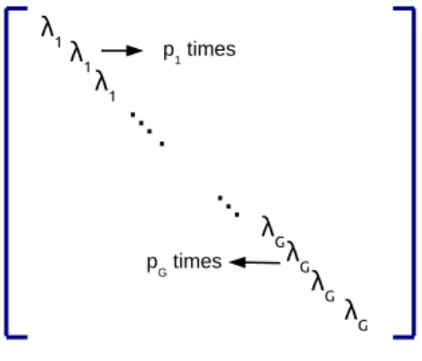
3.2. The Λ matrix . . . 50

3.3. Hierarchical model for Bayesian Group-Lasso . . . 51

3.4. Prior distribution over β . . . 53

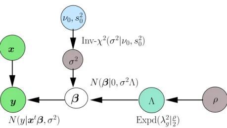
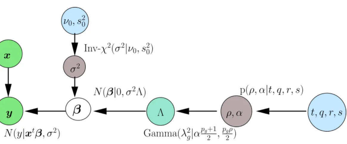
3.5. Hierarchical model for Bayesian grouped-variable selection . . . 53

3.6. Trace plot for coefficients . . . 57

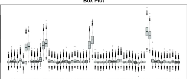
3.7. Box plot for toy experiment . . . 57

3.8. Significance plot for toy experiment . . . 58

3.9. Correlated variables - plots . . . 59

4.1. Random intercept model . . . 62

4.2. Random intercept model for grouped variable selection . . . 63

4.3. Design matrix for categorical variables . . . 64

4.4. Hypergraph illustration . . . 66

4.5. Tissue microarray analysis . . . 71

4.6. Kaplan-Meier curve for breast cancer patients . . . 72

4.7. Distribution of protein expression levels for breast cancer patients . . . 73

4.8. Significance graph for high and low risk patients . . . 74

4.9. Trace plot for 1st order interaction . . . 75

4.10. Solution path for Group-Lasso with Poisson likelihood . . . 76

4.11. Bayes nets plots using deal package . . . 77

4.12. Illustration of a 50 splice site . . . 78

4.13. MEMset data - distribution of A,C,T and G . . . 79

4.14. Interaction patterns from Poisson regression . . . 80

4.15. Interaction patterns from binomial regression . . . 80

5.1. Dummy coding illustration . . . 86

5.2. Mixture-of-experts model . . . 88

5.3. Hierarchical model for survival analysis . . . 90

5.4. Simulation results . . . 96

5.5. Kruskal-Wallis rank test . . . 97

5.6. Significance graph for survival analysis . . . 98

(14)

6.1. Annealing illustration . . . 103

6.2. Plots for the conditional prior distribution overβ . . . 109

6.3. Lasso solution path for diabetes data . . . 113

6.4. Annealing plots for diabetes data . . . 114

6.5. Flexible sparsity experiment . . . 115

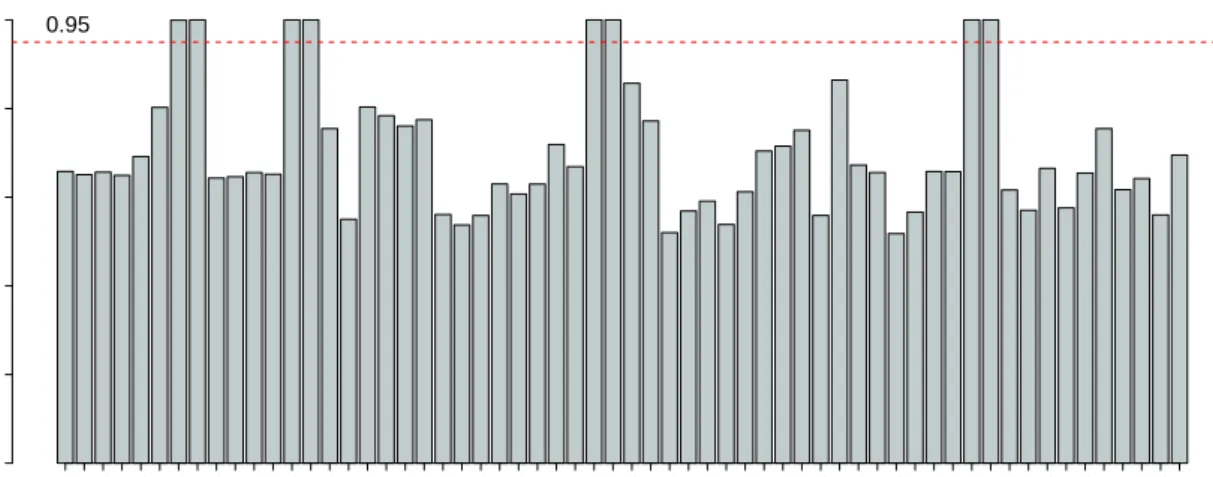
6.6. Box plot of the group norms for MEMset donor dataset . . . 116

6.7. Annealing bar graph . . . 116

6.8. Group-Lasso solution path for MEMset data . . . 117

(15)

If a thing can be done adequately by means of one, it is superfluous to do it by means of several; for we observe that nature does not employ two instruments if one suffices.

Thomas Aquinas

1

Introduction

1.1 Data Analysis with Regression Models

In the realm of data analysis, in a large number of application domains, one frequently encounters applications where one analyzes the relationship between a large number of measurements and the response that they create. These measurements are generically referred to as input or predictor variables and the responses as response variables. More

formally, we can represent this relationship based on the probability distributionp(y|f(x))

where x ∈ _Rd _{represents a} _d_{-dimensional vector variable,} _x _{= (}_x

1, x2, ..., xd) and f is a

function over x which captures the relationship between x and y and the distribution p

models the stochastic nature of this relation. One of the goals of this representation is to

learn the “best” function f using a learning algorithm. The optimality of the function is

judged such that, if for a particularx, a value ofy is generated from the inferred function

then it is as “close” as possible to the true value ofy, also referred to as the ground truth.

Such an optimal function is learned based on given pairs of n observations (xi, yi)ni=1.

Learning such relationships serves the overall purpose of being able to predict responses accurately for new inputs. Such type of learning is also known as supervised learning. Fig 1.1 illustrates the process of supervised learning.

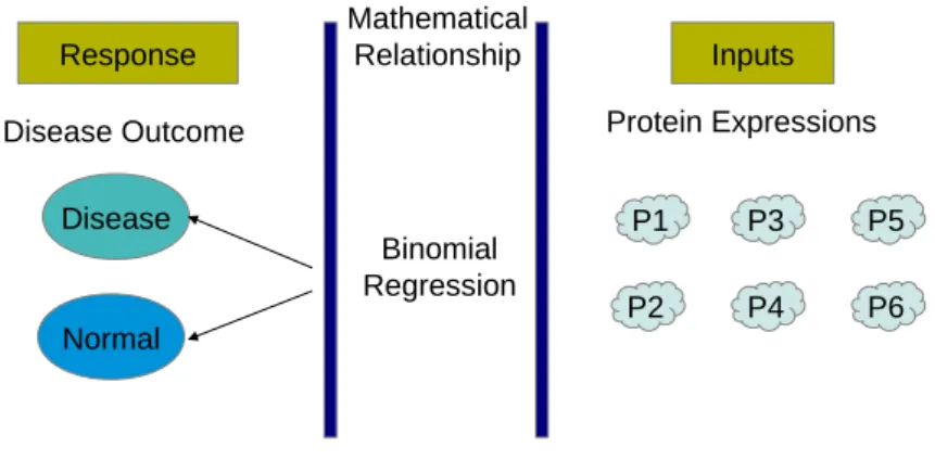
For example, consider a biological example, where the inputs are expression values for various proteins measured from various patients who either have a particular disease or do not. Here the expression values quantify the abundance of proteins produced under a particular experimental setup. The response in this case is a binary variable which can take

values{0,1}where 0 indicates that the patients have the particular disease and 1 indicates

that the patients do not have the disease. The goal is then to learn a distribution which can take the protein expressions as input and accurately predict whether a new patient will have a disease or not. The problem is graphically described in Figure 1.2.

For analyzing such relationships, linear regression models are one of the most widely studied and used models in statistics. Due to its simplicity, it has traditionally been a popular choice for analyzing such relationships between predictor or input variables and a

corresponding output or response variable. Formally, letxrepresent the augmented vector

{1, x1, x2, ..., xd}for ease of representation andydenote a scalar response. The augmented

(16)

Learning Algorithm Observations Inferred Function Supervised Learning Predicted Response New input X,y

Figure 1.1.: A graphical depiction of the supervised learning problem which involves the learning of a relationship between input and response variables. The observa-tions are used by a learning algorithm to produce a distribution which is then used for predicting responses for new inputs.

regression model is then defined as follows:

y=β0+x1β1+x2β2+....+xdβd+=xtβ+, 1.1

where represents a noise variable which models the error in the observed responses. In

ordinary least squares (OLS), the error is assumed to be normally distributed with mean

zero and fixed variance. Given n observations in the form of the rows in the matrix

X = {xt₁, ...,xt_n} and y = (y1, y2, ..., yn) the goal of finding the “best” function is now

interpreted as finding the optimal regression coefficients β which minimize the disparity

between predicted and observed responses which is represented in terms of a cost function. To find the optimal value of the regression coefficients, it is necessary to define a way to measure the disparity between observed and predicted responses. In the case of OLS, it is the sum of squared difference between the observed and predicted response. The resulting optimization problem is then written as:

ˆ β= argmin_β n X i=1 (yi−xtiβ) 2_. 1.2

In chapter 2, we will look at more generalized versions of the OLS model. So far we have described an optimization based view of data analysis. In section 1.2, we briefly describe an alternate view of data analysis which is probabilistic in nature.

1.2 Bayesian Inference

In the previous section, we saw how a linear regression problem was formulated as an optimization problem for finding the optimal value of the regression coefficients. This was done based on minimizing a cost function which was the sum of squared difference in the

(17)

1.2. BAYESIAN INFERENCE Response Inputs Disease Normal Protein Expressions Binomial Regression Disease Outcome Mathematical Relationship P1 P3 P2 P5 P4 P6

Figure 1.2.: A graphical depiction of a supervised learning problem in biology which in-volves characterizing the relationship between protein expression values and

disease outcome. The relationship is defined using a binomial regression

model.

case of OLS. Another view of the same problem is a probabilistic view. We will briefly explain the various elements of the probabilistic view in the form of Bayesian analysis and what benefits it offers.

Bayesian analysis starts with a prior belief over the parameters (θ) of a model before

any data is observed which may potentially change this prior belief. This is represented

in the form of a probability distribution p(θ) which encodes prior knowledge regarding

the parameters. The prior distribution is very useful in channelizing data analysis in a certain direction. The second component of Bayesian analysis is the likelihood function.

The observations, denoted byD, are modeled by the likelihood function, which quantifies

how well the parameters explain the observed data. The goal is to model the effect of the

observations on the prior belief over θ. Such an effect is modeled using Bayes theorem:

p(θ|D) = p(D|θ)p(θ) p(D) ⇒ ∝ p(D|θ)p(θ), 1.3

wherep(D) is the normalization constant. Using Bayes’ theorem, we obtainp(θ|D), which

is called as theposterior distribution overθ, which is so-called since it models the posterior

belief in θ based on observed data. In the regression problem defined in the previous

section, the parameters are the regression coefficients β. For the case of regression, the

posterior distribution can be written as:

p(β|y, X)∝p(y|X,β)p(β). 1.4

After having defined such a probabilistic interpretation of parameter learning, various quantities of interest can be learned from such a formulation. As in the optimization view,

(18)

This optimal value is known as the maximum a posteriori (MAP). This has an equivalent interpretation in the optimization based view where one seeks an optimal value. But the Bayesian formulation need not only provide a point estimate in the form of the MAP. Since the whole posterior distribution is modeled, other estimates can also be potentially generated like estimating the expectation and the variances of the regression coefficients. Hence, in summary, a Bayesian formulation is potentially beneficial since it can summarize the posterior distribution over the regression coefficients using the moments and the mode of the distribution. Information such as variances are especially useful in quantifying the uncertainty in estimates for the regression coefficients.

So far we have discussed the formulation of linear regression using both an optimization based view and a probabilistic view. We started with the intention of defining a relation-ship between inputs and response with the goal of accurately predicting responses for new inputs. We now look at a different goal of data analysis with respect to the input-response relationship.

1.3 Parsimony in Data Analysis

In the previous section we discussed the relationship between inputs and response with the goal of predicting responses for new inputs. But this need not be the only goal of analyzing such relationships. An alternate goal is the interpretation of the inferred relationship in terms of the significance of each input variable in predicting response. This is done with the intention of selecting a smaller subset of input variables which are considered more important than the others. Such a problem of identifying significant variables which help in characterizing the relationship between the inputs and the response is known as feature selection or variable selection. We shall call such a model a parsimonious or sparse model, since a sparse set of variables are selected.

The need for a parsimonious model via feature selection is motivated in multiple ways. The first factor influencing such a need is the possibility of existence of a natural redun-dancy in the underlying data. This can easily be the case in a lot of application domains where the starting point of testing a hypothesis involves looking at all possible variables that could effect the understanding of a certain hypothesis. Then, through suitable data analysis, an attempt is made to find the truly important variables which contribute to the understanding of underlying pattern in data. From an application perspective, this reduces future cost of data collection since only the significant variables identified by the data analysis step need to be measured.

But cost is not the only gain in a parsimonious model. Another very important mo-tivating factor involves the interpretation of the input variables with respect to the real world problem being analyzed. Although a large number of variables may enhance the quality of data analysis for a particular application, such models are often too complicated to understand and interpret. Hence, it becomes useful to reduce the variable set in order to build a more understandable model of the real-world application being studied. This type of a parsimonious approach helps application domain practitioners to gain a deeper understanding of the problem being studied. This may potentially lead to designing of

(19)

1.3. PARSIMONY IN DATA ANALYSIS

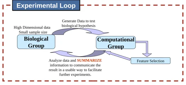
novel hypotheses which are tested through further experiments. Such experiments then produce more data which may again involve a similar type of data analysis. We will call such a cycle of real-world experiments triggering data analysis and vice-versa an experi-mental loop. A good part of the work described in this document is motivated from this experimental loop where it becomes essential to communicate the results of data analysis in a way that it can be interpreted and utilized further for triggering further research in the particular application domain. A graphical depiction of the experimental loop is shown in Figure 1.3.

Biological

Group

Computational

Group

Generate Data to test biological hypothesis

Feature Selection Analyze data and SUMMARIZE

information to communicate the result in a usable way to facilitate

further experiments.

Experimental Loop

High Dimensional data

Small sample size

Figure 1.3.: A graphical depiction of the experimental loop which starts with data col-lection from a real-world application, for example analysis of data produced from biological experiments. This data is then passed on for analysis to a computational group. The analysis in this case is the generation of a sparse model. Based on the requirements, a final summary of the analysis is given back to the domain practitioners leading to further experiments which may lead to further experiments and data generation.

To explain with an example, in the biological problem of predicting disease outcome as mentioned earlier, a biologist who analyzes such a problem may not be interested only in the prediction accuracy of the model, but also in a deeper understanding of the role each protein plays on the disease outcome. The identification of a small subset of more significant proteins may trigger further analysis of the biological interpretation of how the disease is caused.

In this work, we focus on the goal of interpretation in the context of linear regression models via variable selection. We will describe some existing methods of variable selection in linear regression models and identify some of their shortcomings. We will then present our extended framework for variable selection with applications primarily in the biological domain. Although in this work, we focus on biological applications, the ideas presented

(20)

here can be applied to other application domains like image and text analysis. In the next section, we briefly describe some of the biological application areas which present the opportunity to apply variable selection methods.

1.4 Application of Sparse Models in Biology

In this section, we will give a preview of some of the application scenarios which will be used for analyzing real-world data in the context of models that we will discuss in subsequent chapters.

Protein Expressions in Tumor Analysis. A common type of data collection in biology

is related to measuring protein expressions using tissue microarrays (TMA). A tissue microarray is used for the screening of genetic or protein markers across different samples as opposed to DNA (Deoxyribonucleic acid) microarrays which help in studying expressions of thousands of genes simultaneously. Tissue microarrays are often used for tumor analysis and are based on tissue or serum samples collected from patients affected by the tumor. Each array has patient specific histological samples from tumor infected tissues. The resulting TMA slides are then subjected to techniques like immuno-histochemsitry or in situ hybridization based on the specific type of analysis involved.

Due to the high throughput nature and cost-effectiveness of the tissue microarray tech-nology, it is a preferred choice for identifying tumor related biomarkers. Biomarkers are generically used as indicators for a particular biological state. In this case, the idea is to measure protein expressions using TMAs to identify a small set of significant proteins which play an important role in tumor analysis. The identification of such proteins or biomarkers has the potential of furthering proteomics research by providing a better un-derstanding of the underlying biological processes which result in the observed phenomena. We shall show in subsequent chapters that the problem of biomarker detection using data collected from TMAs can be formulated as a variable selection problem in linear regression models where the variables represent the expression values of different proteins. Parsimonious models or sparse models are ideally suited for this purpose, since the goal is not only to predict a particular biological phenomena, but also to provide interpretation in terms of identifying significant proteins.

Splice Site Detection. Another type of analysis in biology is related to the DNA of

an organism, which codes instructions useful for the functioning of an organism. It can be regarded as a long string of characters, where the characters are chosen from the

alphabet {A,C,T,G}, like for example ”ACAATTGGCTAAAAAACCGTTTGCACGA”.

Each character represents a particular type of nucleic acid, where A - Adenine, C-Cytosine, T- Thymine and G-Guanine. These long chains of nuclei acids are responsible for the inner workings of an organism. Within such long strings are sections known as genes which are responsible for production of proteins which in turn perform a particular function. There are two types of sub-sections within these sections which are of specific interest, namely

(21)

1.4. APPLICATION OF SPARSE MODELS IN BIOLOGY

the exon and the intron, which alternate in a given DNA sequence. A splice site is the position(s) in the DNA which separates an intron from an exon. splice

The exons are the functional parts of the gene which are used to produce proteins. During the protein generation process, the introns are identified and discarded. In order to identify the exons and introns in a gene, a problem which is encountered is the difficulty in determining which positions are genuine splice sites. One way of tackling this problem is to infer an identification rule based on the content of the neighboring positions. A further step in this inference can be to identify which neighboring positions (or combinations of positions) are important in assessing the authenticity of a splice site. This type of analysis can then give the biologists insight into the biological reasons behind the existence of these sites and their positioning in the DNA. In later chapters, we analyze this problem using the MEMset human splice site dataset which consists of annotated splice information for a large number of sequences from the human DNA. The goal of data analysis is to use the existing annotation to detect the positions which are instrumental in distinguishing between a true and a false splice site.

Survival Analysis for Breast Cancer Patients. In biology, survival analysis problems

generally involve the modeling of survival patterns of a group of patients based on a disease being analyzed. A survival pattern refers to the distribution of survival time where the meaning of “survival” can be interpreted in different ways based on the specific application. Usually, the experiment setup involves a common theme between the group of patients under consideration, for example the patients may be suffering from a particular disease and are all treated with the same medicine. In such a case survival time can be interpreted as the time till a patient does not have a re-occurrence of the disease.

The data that is collected in such a case involves survival time along with some other measurements like clinical data and gene/protein expressions. The collected data can then be analyzed in multiple ways based on the biological hypotheses being tested. The first aspect of analysis involves identifying possible sub-groups within the patient group based on the differences in their survival patterns. Identifying such differences can help in looking at the possible reasons for certain patients to have a more desirable survival pattern than some other patients and can also be useful from the perspective of personalized medicine or targeted therapies.

Another aspect of analysis can involve relating the survival patterns with the other available measurements such as clinical data and gene/protein expressions. As mentioned before, the interpretation of this relation in terms of identifying significant measurements may lead to a better understanding of the biological reasons which give rise to certain survival patterns. In this work, we look at the specific survival patterns of breast cancer patients and identify low-risk and high-risk patients through clustering. Simultaneously we identify significant proteins which can serve as bio-markers for characterizing survival patterns in patients.

(22)

1.5 Outline and Contributions

After giving a brief introduction of some of the ideas and applications related to sparse models in linear regression, we now give a more detailed roadmap of how this thesis is organized in the next few chapters. The central theme of this thesis is the description of a general framework for Bayesian grouped variable selection in the context of linear regression models. The various components of this framework are then developed which justify its generality and applicability to a variety of modeling scenarios.

In Chapter 2, we review some concepts and terms related to linear regression in detail and then describe some of the existing literature in the field of variable selection. The description is divided into two parts. The first part looks at an optimization based view of the problem and the second one looks at a Bayesian view which builds the motivation for our Bayesian framework for grouped-variable selection.

In Chapter 3, we describe the main goals of this thesis followed by a description of the Group-Lasso. Using the Group-Lasso and the Bayesian Lasso as motivation, we build a Bayesian framework for grouped variable selection which we call the Bayesian Group-Lasso. The full hierarchical model is presented along with the inference procedure in the form of Markov Chain Monte Carlo sampling. We further generalize Bayesian Group-Lasso to a variable selection framework which has an extra parameter to enforce various levels of sparsity without causing excessive global shrinkage of the regression coefficients. In Chapter 4, we add a component of simulated annealing in order to provide another estimate in the form of a point estimate of the regression coefficients by estimating the mode of the posterior. This extension is formally justified by using a variational formula-tion approach.

In Chapter 5, we move beyond simple linear regression and extend the model to gen-eralized linear mixed models so that the framework can cater to different types of data analysis problems. Two specific examples, namely the Poisson regression and binomial re-gression are discussed in detail with demonstrations on real-world biological applications. In Chapter 6, we discuss another application, namely survival analysis and describe how it fits into the generalized linear model framework. Further, through this model, yet another extension to the framework is described by creating a clustering component for simultaneous inference of sub-groups (clusters) and respective significant features in each cluster. This is done by using a infinite mixture-of-experts model.

Finally, in Chapter 7, we discuss the overall thesis in the context of other parallel

developments in the field of Bayesian variable selection in order to give an overall sum-mary of these methods. We also discuss possible future work and extensions to the work described here.

The following publications have resulted out of the work presented in this thesis:

“The Bayesian Group-Lasso for analyzing contingency tables.” Sudhir Raman,

Thomas Fuchs, Peter J. Wild, Edgar Dahl, Volker Roth. ICML’09: Proceedings of the 26th international conference on Machine Learning, pages 881-888, 2009.

(23)

1.5. OUTLINE AND CONTRIBUTIONS

“Sparse Bayesian regression for grouped variables in generalized linear models.”

Sud-hir Raman and Volker Roth. Pattern Recognition: 31st DAGM Symposium, Lecture Notes in Computer Science 5748, pages 242-251, 2009.

“Infinite mixture-of-experts model for sparse survival regression with application to

breast cancer.” Sudhir Raman, Thomas J Fuchs, Peter J Wild, Edgar Dahl, Joachim M Buhmann, Volker Roth. BMC Bioinformatics 2010, 11(Suppl 8):S8 (26 October 2010).

“MAP estimation via simulated annealing for sparse Bayesian regression using MCMC

sampling.” Sudhir Raman and Volker Roth, Monte Carlo Methods for Modern Ap-plications Workshop @ NIPS 2010.

(24)

(25)

2

Variable Selection in Linear Regression

Models

2.1 Introduction to Linear Regression Models

In this chapter, we lay the foundations for variable selection in linear regression models. We will first begin by describing the general setup of linear regression and then will briefly review the literature on variable selection from an optimization perspective. Finally, we will look at the Bayesian formulation of the variable selection problem in order to motivate our contributions described in the next few chapters.

A linear regression framework is defined based on the association between ad-dimensional

vectorx∈_Rd_{known as the input or the predictor variable and a corresponding real-valued}

scalar y∈ _R known as the response variable. The relationship between the two variables

is defined based on a linear function:

y=φ(x)tβ, 2.1

where φ(x) is a vector of d functions (φ1(x), φ2(x), ..., φd(x)) which are known as basis

functions,β = (β1, β2, ..., βd) are the parameters of the model known as regression

coeffi-cients and the use of the word “linear” indicates linearity of the function with respect to the regression coefficients. Since observed data is generally associated with noise, an error

term is introduced to model the stochastic nature of the variable y:

y=φ(x)tβ+, 2.2

whereis a random variable whose distribution is fixed based on the problem at hand. In

this work, we do not consider the modeling of the distribution over the predictor variables

x except when we build clustering models in the the context of survival analysis. The

discussion of these models will be postponed till chapter 5. The linear regression model

can be interpreted in a probabilistic framework by modeling the distribution overy:

y|x,θ,β∼p(y|φ(x)tβ,θ), 2.3

where θ represents all the other parameters of this distribution which we assume to be

(26)

are independent and identically distributed (i.i.d), our goal is to find the value ofβ which best explains the observations in terms of the model defined above. This is done by defining a likelihood function: L(β) = n Y i=1 p(yi|φ(xi)tβ,θ), 2.4

where the likelihood quantifies how well the data is explained based on the given parameter

β. The goal of inference is to find the parameter β which best explains the data or more

specifically which maximizes the likelihood function. The resulting optimal value of β,

denoted byβ_{M L}, is known as the maximum likelihood estimate:

β_{M L} = argmax_β L(β). 2.5

Since the logarithm function is a monotonically increasing function of its argument, max-imizing a function is equivalent to maxmax-imizing its log or minmax-imizing the negative log. Hence, maximum likelihood estimation can be rewritten as a cost or loss minimization problem by taking negative logarithm of the likelihood:

β_{M L} = argmin_β C(β), 2.6

where C(β) = −ln(L(β)) is referred to as a cost or loss function and “ln” denotes the

natural logarithm function. Hence eq. (2.5) and eq. (2.6) represent two views of the same optimization problem.

Ordinary Least Squares Problem. A special case of the above defined linear regression

model is the ordinary least squares (OLS), in which the basis function vector isφ(x) = x

and the error on the response variable is normally distributed, y ∼ N(y|xtβ, σ2), where

N(•|µ, σ2_{) denotes a normal distribution with mean} _µ _{and variance} _σ2_{. From eq. (2.6),}

the optimization problem for OLS is written as:

β_{M L} = argmin_β ky−Xtβk2₂, 2.7

where y = (y1, y2, ..., yn) is a n-dimensional vector of responses and X is a n×d matrix

with rows (xt

1,xt2, ...,xtn) representing the n inputs. We will refer to this loss function as

the least squares loss function.

2.2 Regularization in Linear Models

In a more abstract setting, we can look at parameter estimation from the perspective of optimizing a functional in order to estimate an optimal function which minimizes a given cost functional. The space of functions over which this optimization is done is known as the hypothesis space. In the case of linear regression, the hypothesis space is the space of all

linear models. In linear regression, we infer the “best” function or the optimal value forβ,

(27)

2.2. REGULARIZATION IN LINEAR MODELS

The objective of inferring such a function is to be able to generalize the relationship between inputs and response for unseen data so that it helps in predicting responses for new inputs where the true responses are missing. This notion of generalization can be quantified by measuring the error made in predicting responses for all unseen data. The lower the error, the better is the generalization capacity of the inferred function.

Formally, this is measured as the expected loss on the entire data space (x, y):

R =Ey,x[C(β)], 2.8

whereE denotes the expectation function over the distributionp(x, y). We do not usually

have access to the entire data space and only a smaller set of observations are available. Hence, in practice, we find the optimal function based on the given observations by using an approximation to the expected loss, in the form of the empirical loss function:

Remp= 1 n n X i=1 C(β). 2.9

To address the issue of measuring how well the inferred function generalizes over unseen data, the entire set of observations is divided into a two parts: training data and test

data. Training data is used for finding the optimal value ofβ by minimizing the empirical

loss function using only this data. Once the optimal value of β is found, the test data

consisting of m observations, is used as unseen data to measure how well the inferred

parameters predict the responses by again using the empirical loss function with the test data. The empirical loss for training data is known as the training error. The empirical loss for test data is known as prediction or test error and it serves as an approximation to the generalization capacity of the model.

A common problem that is faced in functional optimization is to decide how rich the hypothesis space should be in order to generalize well over unseen data. If the hypoth-esis space allows a very rich set of functions, it tends to generate a lower training error. Hence the resulting optimal function is said to “fit” the training data quite well. But the downside of this is the possibility of simultaneously increasing the prediction error, since the estimation is finely tuned specifically for training data. This phenomenon is known as over-fitting. The reverse problem involves choosing a very restricted hypothesis space which results in under-fitting the training data due to a restricted choice of functions. A common strategy to such problems is to build a hypothesis space in such a way that there is a balance between over-fitting and under-fitting and this process is called regularization. In the context of linear regression models, to avoid such problems, regularization is

carried out by imposing further constraints on β. One of the most common forms of

regularization in regression involves adding a constraint on the `p-norm of regression

co-efficients: β_RL = argmin_β C(β) s.t. kβkp ≤κ, 2.10

where `p norm of β or kβkp is defined as (P_i|βi|p)

1

p. This above form of constrained

(28)

of the optimization problem: β_RL = argmin_β (C(β) +ckβkp), 2.11

where c is the Lagrangian parameter which tunes the amount of regularization in the

model. Setting it to zero gives us back the non-regularized version of the problem which may lead to over-fitting whereas setting it to a large value can lead to under-fitting. We will use both the constrained and penalized forms interchangeably in the rest of this document. A specific case of penalized linear regression is ridge regression, which penalizes

the`2 norm. For a least squares loss function as in the OLS, the ridge regression problem

is written as: argmin_β ky−Xβk2 2 s.t. kβk2 ≤κ. 2.12

In linear regression models, the concept of regularization can be viewed in a probabilistic

framework as a prior imposed on the regression coefficients β. For the model defined in

eq. (2.12), the prior over β is a normal distribution. The full probabilistic model can be

described as: Likelihood: y ∼N(y|Xβ, σ2I) Prior: β ∼N(β|0, τ−1). 2.13

Using Bayes theorem, the posterior distribution overβ is written as:

p(β|y, X, σ2, τ−1)∝N(y|Xβ, σ2)N(β|0, τ−1). 2.14

With the introduction of the prior distribution, the problem of maximizing the likelihood changes to the problem of maximizing the posterior distribution over regression

coeffi-cients. The resulting optimal value for β is known as the MAP(maximum-a-posteriori)

estimate. Taking negative logarithm of eq. (2.14), we get back the penalized version of

the optimization problem as in eq. (2.12). Hence the MAP estimate ofβand the solution

to eq. (2.12) are equivalent for specific values of the hyperparameters.

Likelihood Models. We now turn our attention back to the likelihood functions or

equiv-alently the loss functions in linear regression models. In this work, we will focus on

likelihood functions which are based on the exponential family of distributions. The ex-ponential family of distributions consists of distributions which share a common form and is generically defined as:

f(x|θ) = h(x) exp[η(θ)Γ(x)−A(θ)], 2.15

whereθis the parameter of the distribution. This form includes most of the commonly used

distributions like normal, gamma, Poisson, binomial distributions etc. The exponential family of distributions are log-concave and hence the corresponding loss functions obtained by taking negative logarithm are convex. Hence, optimizing these functions result in

(29)

2.2. REGULARIZATION IN LINEAR MODELS

problems as long as the constraints result in feasible regions which are convex. For the rest of the document, while referring to likelihood or loss functions, we would implicitly assume that the likelihood function stems from the exponential family of distributions.

Generalized Linear Models. Till now, we have discussed linear regression models in the

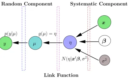
context of response variables which are real-valued scalars. To broaden the applicability of linear models to other types of response variables like binary values or count data, these models can be extended in a way that maintains the linear effect of the predictor variables. This is done by defining a generalized linear model (GLM). A GLM consists of three components, as described in [1]:

1. Random component: The response variable y is the stochastic component which is

distributed according to some distribution with mean µ. This component is

some-times also referred to as error structure orresponse distribution.

2. Systematic component: η = xt_β _{is the systematic component producing a linear}

predictor. So the explanatory variables x affect the response variable y, through

a function of η. The two assumptions implicit in this component are the additive

effects of the variables and linearity of effects.

3. Link function: It specifies a function which connects the mean of the distribution describing the response variable (typically an exponential family distribution) to the

systematic component, as g(µ) =η.

β

η µ σ2 x y Random Component Link Function Systematic Component N(η|xt_β_{, σ}2₎ g(µ) =η p(y|µ)

Figure 2.1.: Dependency structure of a random intercept model (i.e. a GLM with a stochastic systematic component). The dotted blocks represent the differ-ent compondiffer-ents of the model indicating which variables are part of that block by touching the relevant connecting arrows.

Further, we can extend the standard definition of the systematic component by adding a

(30)

Table 2.1.: Commonly used likelihood functions for generalized linear models.

Response variable Distribution Commonly g−1(η)

Used Link Function

y ={0,1} Bernoulli Probit Φ(η) = cdf of

a Normal dist.

y= (0,1,2, ...) Poisson Log exp(η)

y= (−∞,+∞) Gaussian Identity η

deviations making the model more flexible with respect to finding the effect of variables

xon the response variable y. This is described as follows:

η =xtβ+, where ∼N(0, σ2). 2.16

The three components of a GLM together with the random effect constitutes the simplest form of a generalized linear mixed model (GLMM) with a random effect as an intercept term, known as a random intercept model. A graphical representation of all the compo-nents of a random intercept model is shown in Figure 2.1. In the rest of the document, any reference to GLMs will be treated as a reference to the random intercept model. The full probabilistic model is written as:

p(y|θ) =h(y) exp[yθ−A(θ)] E(y|θ) =µ g(µ) =η p(η|x,β, σ2) =N(η|xtβ, σ2), 2.17

where p(y|θ) is the likelihood which can be replaced by any exponential family of

distri-butions (normal, Poisson, binomial etc.) based on the choice of modeling for the target

variable y. Some examples of the commonly used distributions (which are also used in

subsequent chapters) and their link functionsg(·) are given in Table 2.1. In later chapters,

we will see how the component structure of GLMs is used to extend our Bayesian frame-work for grouped-variable selection to specific models like Poisson and binomial model with minimal changes to the overall framework.

Towards variable selection. Although we have discussed the notion of regularization in

the context of improving the generalization capability of the inferred model i.e. achieving low prediction error, there is another aspect of regression that is not suitably addressed by models like ridge regression. The other aspect of inference in linear models is the interpretation of the solution. Interpretation in this context refers to quantifying the significance of the predictor variables in predicting the response. While dealing with a large

(31)

2.3. SINGLE VARIABLE SELECTION IN LINEAR REGRESSION MODELS

set of predictor variables, it is often desirable to select a small subset of significant variables which have a stronger effect on the response variable and perform regression with these variables. This is especially true from an application perspective, where a domain expert may not only be interested in good prediction accuracy, but also in understanding some of the more important effects of inputs on response. The identification of such important predictor variables may lead to a further understanding of the real-world problem being analyzed. Also in keeping with Occam’s razor which postulates that all things being equal, a simpler explanation is preferable to a more complex one, it is more desirable to explain the model with a smaller set of variables. The process of identifying significant variables is known as variable selection or feature selection. In linear regression models, the variable selection process involves the estimation of the regression coefficients for the significant

predictor variables. This can be further interpreted as obtaining a sparse β vector which

indicates significance of a variablexi if the corresponding coefficient valueβi is non-zero.

For variable selection, the `2-norm regularization in linear models does not suffice since

it does not encourage sparsity in the optimal values for the regression coefficients. Hence separating out the more significant variables from lesser significant ones is more difficult

in this case and requires an extra selection step after obtaining the β estimates. In the

next section, we discuss various methods that have been proposed to address the problem of variable selection.

2.3 Single Variable Selection in Linear Regression Models

First, we consider a simpler case of single variable selection, in which we assume that there is no a priori knowledge of structural associations between the predictor variables. Although there is a vast literature on variable selection, we will primarily focus on the Lasso (least absolute shrinkage and selection operator) in detail since it lays the foundation for the work that we describe in this thesis. However we will first briefly mention a couple of more methods.

Forward Selection. This method falls under the category of greedy approaches which

select a subset of significant predictor variables. The method is primarily motivated by the

fact that a brute force method would involve checking all the 2d _{combinations of variables}

for judging the optimal feature-subset and the computational complexity grows

exponen-tially with increasingd whered is the number of predictor variables. In forward selection,

we start with an empty “selected-variables” setS which represents the variables that have

been selected so far. Now, for d variables from which we have to select the relevant

sub-set, d linear regression models are learnt containing one variable each. This is done by

minimizing the loss function with only one variable in the equation. After obtaining the parameter values, the model that performs best in terms of prediction accuracy is chosen,

which in turn means that the corresponding variable is chosen and added toS.

In the next step, the same procedure is repeated by pairing the chosen variable with

all the remainingd−1 variables. This results in adding another variable to the

(32)

the best pair was chosen since not all d(d−1) pairs were considered. This procedure

continues to add features sequentially to S till a stopping criterion is met. The stopping

condition can be, for example, a maximum number of variables to be selected or a minimum prediction accuracy to be attained. Another similar approach is backward elimination which is the reverse of forward selection. Here, we start with a full selected-variables set

with all thed variables and then drop variables one by one using a similar procedure as in

forward selection. Since the process of selection is greedy in nature for both approaches, it makes them less robust since the solution tends to be sub-optimal.

Non-Negative Garrote. The non-negative garrote introduced in [2] formulates the

vari-able selection problem in the form of a two step optimization problem which tends to

produce solutions that are sparse in β. The non-zero elements of the resulting sparse β

vector indicate that the corresponding predictor variables are selected. Hence such a for-mulation simultaneously infers the regression coefficient values and selects the significant variables.

The non-negative garrote is formulated as a two-step optimization problem. In the context of a least squares regression problem, the first step of the method involves solving the OLS problem in eq. (2.7) for the regression coefficients. After obtaining the OLS

estimates ˆβ0, the second step defines an optimization problem which selectively shrinks

the OLS estimates and hence tends to produce sparse solutions in β. The second step is

specified as follows: ˆ c = argmin_c ky−X( ˆβ0◦c)k2 2 s.t. cj ≥0∀j, kck1 ≤κ, 2.18

where ˆβ0 is the OLS estimate and the “◦” operator denotes element-wise multiplication.

The garrote is initialized with the OLS estimate and then shrinkage of coefficients is

induced by applying an`1 norm constraint which tends to produce a sparsec vector. The

final solution is (ˆc◦βˆ0). Since the non-negative garrote depends on OLS estimates, it

cannot be used for the case when d > n. However a modification of the non-negative

garrote has been suggested in [3], where the initialization is done based on ridge regression

rather than OLS in order to deal with the case ofd > n. Since the non-negative garrote

is formulated as a two-step optimization problem, it is difficult to obtain a probabilistic interpretation of the problem. We now look at a more compact representation of the variable selection problem which further motivates a Bayesian interpretation.

Lasso - Least Absolute Selection and Shrinkage Operator. Inspired by the

non-negative garrote, a more compact representation of the overall optimization problem is introduced in [4] known as the Lasso. The key objective of the Lasso is the continu-ous shrinking of the coefficients to produce some zeroed out coefficients. Similar to the non-negative garrote, this is achieved by an optimization problem formulated as follows:

ˆ β= argmin_βky−Xβk2 2 s.t. kβk1 ≤κ, 2.19

(33)

2.3. SINGLE VARIABLE SELECTION IN LINEAR REGRESSION MODELS

wherek·k1 denotes the`1 norm. Rewriting it in the Lagrangian form, it can be represented

as a penalized likelihood problem: ˆ β = argmin_β(ky−Xβk2₂+ckβk1), 2.20

where crepresents the Lagrange parameter. The Lasso is also a special case of the more

generalized penalized regression problem also called as bridge regression introduced by [5]: ˆ β= argmin_β(ky−Xβk2 2+ckβkq), 2.21

where q ≥ 0. The special case of q = 1 represents the Lasso and q = 2 is the ridge

regression as defined in eq. (2.12). Another similar model known as the basis pursuit (see [6]) addresses the problem of overcomplete representations, or in other words cases where the number of basis functions exceeds the number of samples. It is almost identical to the Lasso, the only difference being that the loss function and the constraint are reversed:

ˆ β= argmin_βkβk1 s.t. y=Xβ. 2.22

More generally, we can formulate the Lasso for a generic set of likelihood functions: ˆ β = argmin_β(C(β) +ckβk1). 2.23

Since we are considering only the exponential family of likelihood functions, the Lasso

formulation is a convex optimization problem which, below a certain threshold of κ, has

a tendency to approach a solution ˆβ which consists of some exact zeros and hence is a

sparse solution. As in the non-negative garrote, the sparse nature of the solution serves the dual purpose of estimating the coefficients and also performing variable selection, where the variables corresponding to the non-zero coefficients are the ones which are “selected”.

Based on eq. (2.21), we also notice that the Lasso (q = 1) is the threshold for q, below

which the problem becomes non-convex. This is due to the fact that all`qnorms withq ≥1

are convex functions and for q < 1 these norms are semi-norms and violate the triangle

inequality and hence are non-convex regions. Hence bridge regression is convex for q≥ 1

and non-convex for q < 1 . The Lasso (q = 1) has been very popular since it can be

solved using convex optimization techniques without running into issues of local minima. A particularly fast implementation is available in the form of least-angle regression (LARS package in R), see [7]. The motivation behind using the Lasso for a Bayesian interpretation also follows from its compact representation which is easily formulated in a probabilistic setting as a product of likelihood and prior.

Model Selection. The Lasso formulation has an extra parameter c which is the

La-grangian parameter. Till now we considered solving the Lasso problem assuming c to be

fixed. Fixingc to different values gives rise to different models. Hencec can be viewed as

a model selection parameter which also needs to be learnt as a part of the inference pro-cedure. Henceforth, we will refer to it interchangeably as a model selection or Lagrangian parameter. This parameter is usually learned via cross-validation. In this procedure, the

(34)

training data is divided into two parts. One part is used to train the model with a fixed

value of cand the other part is used for calculating the prediction accuracy of the model.

For eachc, this procedure is averaged out for different divisions of the training data. After

doing this for a range of values for c, the value that gives least prediction error is chosen

and the full training data is then used to obtain the final Lasso estimates. For different

values of c, the resulting Lasso estimates are plotted in terms of solution paths which

plot how the value of each regression coefficient evolves with the changing values ofc. Each

path represents one regression coefficient. An example of a solution path plot is shown in Figure 2.2. The least-angle regression implementation for the Lasso in [7] exploits the

0.0 0.2 0.4 0.6 0.8 1.0 −500 0 500 |beta|/max|beta| Standardized Coefficients LASSO tc sex ltg bmi ldl tch map age hdl glu

Figure 2.2.: Plot of the Lasso solution path generated with diabetes dataset (see [7]) using the LARS R package which contains a standard Lasso implementation. Each path represents the trace of the values taken by a particular coefficient for

increasing values of κ.

fact that the solutions paths for the Lasso are piece-wise linear. This results in significant computational gains as the solution paths can be computed very efficiently.

Standard Error Estimates. As discussed in [8], since the Lasso is non-differentiable, it

is difficult to get an estimate for the standard error of the regression coefficient estimates. This is due to the fact that the Hessian is not defined at the optimal solution. An ap-proximation to the covariance matrix of the coefficient estimates from the Lasso has been suggested in [4]. However this approximation works only for the non-zero coefficients. For the zero coefficients, the standard error is estimated to be zero. A better estimate was provided in [9] which worked for the zero coefficients as well but only in the case of

d < n. Bootstrapping is another alternative method for estimating standard error. But as discussed in [8], the bootstrap estimates for the Lasso are not consistent for the zero coefficients. One of the advantages of the Bayesian framework that we present in this work

(35)

2.4. GROUPED-VARIABLE SELECTION

is that we are able to summarize the distribution over regression coefficients with estimates for the moments and the mode by obtaining samples which closely resemble samples from the distribution over regression coefficients.

Another issue with the Lasso is that whenever there exists a group of significant and highly correlated predictor variables, the Lasso tends to select only one variable from the group, since it is redundant to also select all the other variables. In the extreme case of the variables having an exact linear relationship with each other, the variable is randomly chosen from the group. To tackle this issue, another formulation for variable selection via the elastic net has been proposed in [10]. In this work, we see how a Bayesian approach to the problem resolves this issue regarding correlated predictor variables.

2.4 Grouped-Variable Selection

In this section, we will introduce grouped-variable selection briefly and a more detailed de-scription will be given in the next chapter. Although the mechanism for variable selection is introduced via the Lasso, it is still insufficient for problems where the predictor vari-ables have a predefined layer of structural associations which introduces further constraints in the variable selection process. An example of such structural associations is a group structure where the predictor variables are divided into groups and the selection problem involves selecting whole groups of variables rather than individual variables. Hence in the context of regression, the desired solution requires entire groups of related coefficients to be selected (non-zero) or entire groups to be zeroed-out indicating non-selection.

An example of such a group structure which arises naturally is while regressing predic-tor variables which are categorical in nature. The categorical variables are expressed as groups of dummy variables and hence the original problem of selecting significant categor-ical variables transforms into the problem of selecting groups of dummy variables, each group representing a single categorical variable. Another example of a group structure

in regression is the k-th order polynomial expansions of the predictor variables where the

groups consist of products over combinations of variables up to degreek.

Motivated by these modeling scenarios, a grouped variation of the Lasso, i.e. Group-Lasso, is introduced in [11]. The modified least squares penalized optimization problem is formulated as follows: ˆ β= argmin_β(ky−Xβk2 2 +c G X g=1 kβ_gk2), 2.24

where k · k2 denotes the `2 norm, G is the number of groups and βg is a sub-vector of

β which represents all the regression coefficients of group g. The key modification lies

in the penalization which involves an `1-`2 constraint on the regression coefficients. This

penalty encourages sparsity ofβat the level of groups which is represented by the`1 norm

between groups and within groups there is an`2 norm. The above formulation is again a

convex optimization problem.

(36)

proce-dure to efficiently compute all the solutions paths as demonstrated in [7]. However, the Group-Lasso solution path is, in general, not piece-wise linear, hence it requires intensive computation for large-scale problems. A fast active-set algorithm was proposed in [12] to deal with large scale problems. The issue related to non-uniqueness of solutions in Group-Lasso problems is identified in [12] and suitable test is defined for verifying if the solution for the given Group-Lasso problem is unique or not. Also the Group-Lasso has been extended for GLMs in [12]. However, the issue regarding estimation of standard error as discussed in the Lasso case is still carried over to the Group-Lasso as well.

Apart from the group structure, other types of structural associations between predic-tor variables have been modeled, like the fused Lasso [13] which imposes sparsity in the difference between successive coefficients, assuming a certain ordering of the variables. In this work, our focus is only on the grouped variable selection problem although extensions to other variations of structural associations can possibly be thought of along similar lines.

2.5 Flexibility in Inducing Sparsity

In high-dimensional data, an issue often associated with the Lasso formulation is the presence of too many non-zero coefficients in the solution. Using the Lasso, the usual way

to remedy this problem is to shrink the coefficients further by increasing thecparameter

in eq. (2.20). However, since the Lasso is based on global shrinkage of the coefficients, this results in shrinking even the non-zero coefficients, which in turn can effect the predictive accuracy of the estimated regression coefficients.

To address this issue, another version of the Lasso, namely the relaxed Lasso has been

introduced in [14] which introduces an extra parameter φ in the following manner:

ˆ β= argmin_β ky−X{β.1Mc}k 2 2+φckβk1, 2.25

where c ≥ 0 and φ ∈ (0,1] and 1Mc is an indicator function on the set of variables

Mc⊆ {1, ..., d}so that the vector term{β.1Mc}hasdcomponents and for allk∈ {1, ..., d},

each component is defined as:

{β.1Mc}k=

0 k /∈Mc

βk k ∈Mc

. 2.26

This formulation leads to a flexibility in imposing sparsity since the parameter c and φ

separately control variable selection and shrinkage of coefficients.

The algorithm for relaxed Lasso breaks up the estimation into two steps, where the first step is the standard Lasso for producing the solution paths. The second step uses various sub-models along the path and again applies Lasso but with a small penalty parameter

φc where φ ∈ [0,1]. As a result the relaxed Lasso finds the same set of sub-models as

the Lasso but with less shrinkage of the non-zero coefficients. Another similar attempt towards a sparser solution with less shrinkage is the adaptive Lasso (see [15]).

Both approaches are designed so that the problem is still within the realm of convex optimization. An alternate approach can be to use the bridge regression penalization term

(37)

2.6. BAYESIAN INFERENCE

kβkq. For values ofq≤1, the solutions produced would have the tendency to be sparse in

nature below a certain threshold ofκ. Figure 2.3 displays the constraint region for various

values ofq. To produce sparser solutions, one can optionally tune the parameter q along

−5 −4 −3 −2 −1 0 1 2 3 4 5 −5 −4 −3 −2 −1 0 1 2 3 4 5 −5 −4 −3 −2 −1 0 1 2 3 4 5 −5 −4 −3 −2 −1 0 1 2 3 4 5 −5 −4 −3 −2 −1 0 1 2 3 4 5 −5 −4 −3 −2 −1 0 1 2 3 4 5

Figure 2.3.: This plot illustrates the difference in the feasible regions according to the

different `q norms used. Left: Concentric circles with `0.5 norm. Center:

Concentric circles with `1 norm. Right: Concentric circles with `2 norm.

with κ, which gives an added flexibility and hence helps in avoiding excessive amounts

of shrinkage of non-zero coefficients. Inspite of flexibility gains in the model, the overall optimization problem becomes non-convex and hence is harder to solve due to presence of local minima. We shall show in this work that the additional flexibility of adjusting sparsity without excessive shrinkage of regression coefficients can be easily achieved in a Bayesian framework by introducing an extra parameter similar to [14]. In the next section, we shift our focus to Bayesian inference and then move towards a Bayesian framework for variable selection.

2.6 Bayesian Inference

Although the Lasso based approach for variable selection has been very popular, there are still some shortcomings of this optimization based approach. The focus of an optimization based approach is to produce a single point estimate in the form of the MAP estimate. Although various estimates for the standard error have been suggested, they work under restricted conditions and in most cases only for the non-zero coefficients. Secondly,

con-trolling the sparsity of the solution with a single parameterc(in eq. (2.20)) has a side-effect

on the global shrinkage of the regression coefficients which may lead to decrease in predic-tion accuracy. Based on the issues associated with the optimizapredic-tion based framework for variable selection, there is a strong motivation to look at probabilistic approaches in order to overcome these issues. We will first discuss a general setting of the inference mechanism in a Bayesian setting and then discuss a Bayesian approach to single variable selection.

The advantage in using a Bayesian approach for modeling purposes is that it allows the extraction of information about the posterior distribution over the parameters in the model which usually includes estimating the moments and the mode of the distribution. Infer-ence in a Bayesian setting generally refers to analyzing the posterior distribution. With

(38)

non-standard definition of priors and likelihoods, the posterior distribution is generally complex and as a result, quantities like the first and second moments cannot be derived analytically. In such cases, one has to resort to techniques which provide approximations to the desired estimates. One such popular inference mechanism that is used to generate such approximations is the Markov Chain Monte Carlo (MCMC) sampling technique. It involves generating a chain of sample points which under mild conditions, asymptotically converge to samples from the desired distribution. There are other forms of approximation in the Bayesian regim