Open set object recognition

(1)

OPEN SET OBJECT RECOGNITION

A Master’s Thesis

Submitted to the Faculty of the

Escola Tècnica Superior d’Enginyeria de

Telecomunicació de Barcelona

Universitat Politècnica de Catalunya

By

Itziar Sagastiberri Fernández

In partial fulfilment

of the requirements for the degree in

MASTER IN TELECOMMUNICATION’S

ENGINEERING

Advisor:

Elisa Sayrol Clols, Josep Ramon Morros Rubió

(2)

Abstract

Deep Learning is a widely used technique for classification tasks. In practise, the most common classifiers are not useful for certain tasks, as they were developed to work in an environment were the number of classes is bounded in training phase. In this thesis, we present an alternative classifier that is able to deal with data that belongs to new classes during testing time. This type of data, in which the number of classes is not defined, is referred to asopen data. There are some Machine Learning classifiers that have been modified to work with open sets, specially based on SVM. Conversely, in the context of Deep Learning open data is a relatively new area of research. In this thesis we work with OpenMax classifier, showing its improvement when working with open data while also achieving similar results to traditional classifiers for known data.

Resumen

Deep Learning es una técnica ampliamente usada en tareas de clasificación. En la práctica, ciertas tareas no pueden utilizar los clasificadores más comunes, puesto que éstos han sido desarrollados para funcionar en un entorno en el que el número de clases está limitado desde la fase de entrenamiento. En este proyecto, se presenta un clasificador alternativo que es capaz de lidiar con la aparición de datos de nuevas clases durante la fase de prueba. A esta clase de datos, en los que el número de clases no queda definido, se les llama datos abiertos. Existen algunos clasificadores de Machine Learning que han sido ajustadas para trabajar con datos abiertos, sobre todo basadas en SVM. Para Deep Learning, por el contrario, los datos abiertos son un área de investigación relativamente nueva. En este proyecto, trabajamos con el clasificador OpenMax, demostrando su mejora en entornos de datos abiertos, y consiguiendo unos resultados similares a los de los clasificadores tradicionales para los datos de clases conocidas.

(3)

ACKNOWLEDGEMENTS

This research has been supervised by Josep Ramon Morros Rubió and Elisa Sayrol Clols, the advisors of this thesis.

(4)

LIST OF FIGURES

1.1 Gantt diagram of the project . . . 4

2.1 Example of a pooling layer [1] . . . 6

2.2 CNN architecture [1] . . . 7

2.3 Top-5 error results of the winning team each year of the ImageNet chal-lenge [2] . . . 8

2.4 Schematic of a residual block [3] . . . 9

2.5 Dual Tail Fitting [4] . . . 11

2.6 Data and decision bounds for SVM, WSVM, SSVM [5] . . . 12

2.7 Space modeling with NCM vs. NNO [4] . . . 13

2.8 Accuracy of SoftMax vs OpenMax with an Open set and with fooling images [6] . . . 15

2.9 Margin limit calculation . . . 16

3.1 Google Search trends for Keras, Tensorflow and PyTorch . . . 19

(7)

LIST OF TABLES

4.1 Accuracy for SoftMax with different known to unknown ratios . . . 25 4.2 Accuracy for OpenMax with different known to unknown ratios . . . . 27 4.3 Types of errors for OpenMax . . . 27

(8)

NOMENCLATURE

CNN Convolutional Neural Network

CVPR Conference on Computer Vision and Pattern Recognition GPI Image Processing Group

ILSVRC ImageNet Large Scale Visual Recognition Challenge MAV Mean Activation Vector

NCM Nearest Class Mean NNO Nearest Non-Outlier

PDF Probability Density Function PLOS Positively Labeled Open Space RBF Radial Basis Function

ResNet Residual Network

SSVM Specialized Support Vector Machine SVM Support Vector Machine

(9)

CHAPTER 1

INTRODUCTION

1.1

Motivation

In a task of image classification, the purpose is usually to identify the class of an image or an object within the image among several possible classes. An example can be found in medical imaging when trying to identify people who suffer from an specific illness. This images could automatically be classified in regards of the presence or absence of markers for said illness. As the dataset is only composed by medical images, the decision is binary; positive or negative. Here the classification task is clearly determined, but not all classification tasks have these characteristics.

In some problems not all classes present in the data are known beforehand, for such cases it is said that the dataset is an open set. Let’s see an example to better understand this situation. When trying to identify a number of people in images or video recordings the purpose may be to classify them in, for example, 10 different categories; that are the 10 different people interesting for the task . But more people may appear in the image or video, perhaps in the background or with one of the known people. In this kind of situation, the system should also be able to reject those samples that do not belong to any of the 10 known categories. Another common situation is when data used for training does not represent every class that can appear during testing time. Therefore, aside from being able to classify the image among the different set of categories which were present during training, it is evident that it would be useful to add an additional category of unknown. For this reason, some alternatives for the current classification methods have been studied by different research groups.

The most commonly used classification layers either give probabilities of the sample belonging to each class, distance of the sample to the available classes etc. But it is always under the assumption that the sample belongs to one of the known classes. In scenarios with open data the assumption does not apply, as it may also belong to an

(10)

unknown class that is not represented by the data. One of the methods that has been used until now, is adding a threshold to the classification output. It is expected that in the case in which the image is from an unknown class the output for this sample will be low probabilities or considerable distances to all classes. Thus, the image gets rejected and categorised as unknown when adding a threshold to the output. But thresholding has two problems, the first being that all outliers of each class might be rejected and labeled as unknown. The image may be somewhat similar to what the network learnt is a representation of the class, but still slightly differ, so depending on how diverse the class is thresholding does not work very well. The other problem with thresholding is with images that have been specifically built to give a high probability of a class even though, for the human eye, they clearly do not belong to the class. These images are called fooling images.

As the current classification layers have not shown good results when dealing with open sets, we want to test different alternatives.

1.2

Objectives

We first need to define our objectives coming into this work and what we expect to achieve at the conclusion of this thesis.

1. Use a pretrained model to test accuracy with our database that includes unknown classes. We will split the database with different ratios of known-to-unknown classes.

2. Build our own model with the OpenMax approach [7].

3. Improve with the OpenMax method the accuracy we get with the classical SoftMax identifying unknown classes.

4. Compare the results we obtain with OpenMax to the ones with EVM method [8].

1.3

Requirements and specifications

The OpenMax method is expected to get a better accuracy in sets of data that have images of both known and unknown classes without sacrificing the performance in evaluating only known classes.

(11)

Some decrease in the accuracy of known classes is expected, but we should not loose more than around 5% in accuracy. This value is just an estimation we decided based on results of methods dealing with open set. On the other hand, we expect to significantly gain accuracy in unknown classes, at different rates depending on the ratio of known to unknown images.

1.4

Planning

We identified 6 different tasks for the development of the project: 1. Study current techniques for open set classification.

2. Choose base line network to operate with. 3. Extract image features of the data set.

4. Implement OpenMax method to allow open set. 5. Test the code.

6. Document the thesis

We can see how the different tasks were spread through time in the following Gantt Diagram, in Figure 1.1. It should be noted that during testing time we were also trying to make OpenMax work for the face dataset, as well as trying the EVM method [8], another approach to deal with open set problems.

1.5

Deviations from the original work plan

Initially, we were planning on testing this method with face recognition, instead of object recognition, so the database we used was different. The problem was that the library we used to get the features of the faces, dlib [9], was incompatible with the PyTorch libraries we were using. We finally decided to use a different database to be able to use a pretrained network in an easier way and get a proof of concept of the OpenMax method. This also meant we changed the whole network, as the model we obtained for faces was a VGG16 network [10] and we finally used a ResNet50 [3]. However, the main goal remained the same, study the performance of OpenMax compared to SoftMax.

(12)

(13)

CHAPTER 2

STATE OF THE ART

In this chapter we will first analyse different techniques that are used for image classification and some examples of popular networks for this task. After that, we will study the solutions that have been used for dealing with open sets that allow to identify samples from unknown classes. We will not only consider neural networks methods, but other machine learning techniques as well.

2.1

Image classification

Image classification is a task that has been studied for years now with different motivations and methods. Here we will see how to classify images using neural net-works, as the thesis is centred in methods for open set image classification with neural networks.

2.1.1

CNN for image classification

There are different types of architectures of Deep Neural Networks that can be used depending on the type of data to analyse; for example, it is not the same to process images, speech or text. For the processing of images the most commonly used architecture is the Convolutional Neural Network (CNN).

A CNN is one of the different types of networks used for Deep Learning. It consists of a succession of convolutional layers, along with some pooling ones. Convolutional layers are those layers of a neural network that apply a convolution to the input limiting all the connections needed in the classical multilayer perceptron, where neurons of one layer are connected to all the neurons of the following layer.

(14)

Usually, the first convolutional layer is responsible for capturing low level features such as edges, colour, gradient orientation, etc. As the model goes deeper, the layers start learning high level features too and the result is a network with a broader under-standing of the images in the dataset. On the other hand, the pooling layer’s function is to reduce the dimensions of the input data by downsampling it. In 2D input, as images, it would divide the input into blocks of data and compute the average of the values, the L2-norm or the maximum value, depending on the type of pooling applied. An example of Max Pooling and Average Pooling layers is depicted in figure 2.1. With the combination of the convolutional layers and the pooling ones the processed data gets simplified to something that is easier to process but without loosing important features that are needed to represent the image. Throughout the network the ReLu activation function is also applied. This is an activation function used in neural net-works that keeps the maximum value between 0 and the input, meaning, it only keeps positive values. At the end of the network, after the convolutional layers, it is common to introduce a fully connected layer and feed the output of this to the classifier. An overview of the whole architecture can be seen in figure 2.2.

Figure 2.1: Example of a pooling layer [1]

CNNs are perfect for image processing because the convolutions can keep spatial and temporal information. Therefore, instead of analysing the image pixel by pixel as a fully connected layer would do, it can perfectly capture the complex information of an image by relating all pixels with neighbouring ones [11].

In the context of image processing a competition of image classification is held every year, the ImageNet Large Scale Visual Recognition Challenge (ILSVRC) [2].

(15)

Figure 2.2: CNN architecture [1]

When this type of architecture was first introduced by one of the teams, the results greatly improved compared with the other teams and with previous years. The first ever CNN used in the challenge was the AlexNet [12], which had a Top-5 Error of 15.3%, 10 points lower than the runner up method. We can see the decrease in the Top-5 error when Deep Learning was introduced in the graph in image 2.3. The results in green are the ones when CNNs and Deep Learning was used and in orange the human performance. The number of layers in the CNN also kept growing, making the models increasingly deeper and getting better accuracies. This is a result of what was explained before, that deeper layers learn higher level features of images and, consequently, have a better understanding of the images.

Since then, different teams started developing their own CNNs for their submissions. Each year, the winning architecture is deeper than before, that is to say, the number of convolutional layers is larger. In the development of this project, we tried 2 of them; VGG16 for face recognition and ResNet50 for object classification.

2.1.1.1 VGG16

VGG16 was developed by the Visual Geometry Group of the University of Oxford. There are different versions of this network and the number 16 refers to the depth of the network but VGG11, VGG13 and VGG19 versions also exist. The architecture of VGG 16 consists on 13 convolutional layers, 5 pooling layers and 3 fully connected ones, so the number in the name does not take into account pooling layers [10]. One of

(16)

Figure 2.3: Top-5 error results of the winning team each year of the ImageNet challenge [2]

the characteristics of this network is that it uses 3x3 filters for the convolution. This smaller size kernel, compared with the ones used in CNNs before of size 11x11 and 5x5, decreases the number of parameters that the network has to learn. However, this model has more layers than the previous ones and as a consequence more convolutions are applied, so it ultimately covers the same area as the previous architectures even with smaller filters.

2.1.1.2 ResNet50

This architecture will be analysed more in depth in the methodology chapter, but as an overview, this is the first time that the concept of Residual Learningis introduced [3]. Residual Learning helps with the problem of vanishing gradient that appears as the network becomes deeper. As explained before, architectures were becoming deeper so that the network had fewer parameters to learn and in consequence also take a shorter period of time to converge. However, backpropagation, which is the common method used by neural networks to update weights, consists of a gradient based learning method where weights are updated in proportion to the partial derivative of the error. More layers mean more derivatives of usually smaller values as it goes backwards, and this is where the vanishing gradients appear. The idea the authors came up with was that the output of the first layer in a block, not only goes to the following layer, but it is also added to the output of the second one. Each block of layers where this is done is

(17)

called a residual block, and a ResNet consists of several residual blocks positioned one after the other. We can see a representation of a residual block in the figure 2.4 for better understanding.

Finally, the architecture consists on 49 convolutional layers, organised in blocks, and a final fully connected layer at the output.

Figure 2.4: Schematic of a residual block [3]

2.2

Open Sets

Traditionally, datasets used for data analysis consist of a collection of samples that are labeled into a number of classes. When building a model, some of those samples are used for training and others for validation and testing, but the number of classes does not vary. This applies for certain tasks, but for others this closed dataset assumption is not true. The training and validation data will be labeled with a number of classes, but the testing data may be quite open. For cases like these, the method needs to be able to deal with the possibility of the data belonging to a class that is unknown to the system. There are many ways in which this has been addressed until now.

2.2.1

Weibull model and EVT introduction

A number of these techniques, whether neural networks or other methods, use

Weibull models [13] and Extreme Value Theory (EVT) [14] to deal with open set problems, so the basics will be explained now to understand the reason behind it and the techniques that use them. Nonetheless, this topic will be further explained in section 3.4.1, where we will describe how the Weibull models for OpenMax are calculated and how OpenMax uses them.

(18)

A Weibull model is a statistical model based on Weibull distribution, which is typically used to analyse unexpected behaviour of a system. As it can model atypical behaviour, it is also used for EVT, a theory meant to study the deviations in respect to the expected value. This theory is widely used in meteorology and seismology to be able to predict an earthquake or a flooding, but it can be used to study any kind of distribution and its extreme values. As the combination of both, Weibull and EVT, is used to define and examine the extreme values of a model, they are suitable for open set classification to be able to analyse a sample and decide if it belongs to a class but has an atypical value that deviates from the mean, or on the contrary, it belongs to an unknown class.

2.2.2

Previous solutions

First of all, we can have a look at what was done in Machine Learning techniques to work with open sets before neural networks.

2.2.2.1 WSVM

One of the best ways to deal with open sets was with Support Vector Ma-chines (SVM). This is a well known and popular Machine Learning technique that was originally designed for binary classification but it was also successfully extended for multi-class. SVM divides the space with hyperplanes to be able to create sections that belong to each of the classes. However, SVM divides the whole space, which is not interesting for open sets. Thus, based on this there is a method called Weibull-calibrated Support Vector Machine (WSVM) [15] that does not divide all the space and assign it to one of the current classes. The method uses Weibull distributions and EVT to build those hyperplanes and define the areas that belong to each of the classes. The method fits the data to a Weibull model for the probability of the sample of being part of one of the known classes and another one that fits the classes it does not belong to. This method is a dual tail-fitting, as with the knowledge of the distribution of a known class, it also fits the data that does not belong to this class using another Weibull model, and it tries to better define this separation between classes. We can see this dual tail fitting in figure 2.5, where in the left we have the model for the samples that do not belong to the class, and in the right we have the Weibull model for the class.

2.2.2.2 SSVM

Based on SVM there is a second method called Specialized Support Vector Machine (SSVM) [5]. In this method, they ensure a bounded Positively Labeled

(19)

Figure 2.5: Dual Tail Fitting [4]

Open Space (PLOS) by using a Radial Basis Function (RBF) kernel and forcing the bias to be negative. This PLOS that they want to bound is the space where the known categories are represented. For a better understanding of the method, we have below an image, Figure 2.6, showing the different ways in which the decision regions are represented by the different methods. In the first picture (top-left), we can see the real distribution of the data; and on the following one (top-right) how the traditional Support Vector Machine deals with the division of the space. In SVM, as it does not deal with open data, all space is assigned to a class. On the bottom of the picture, we have two methods that can deal with Open Space. We can observe that WSVM generalises slightly better, giving a smoother division of classes as a result of the Weibull model, whereas SSVM fits the data more tightly.

2.2.2.3 NNO

The method of Nearest Non-Outlier (NNO) [16] is based on the Nearest Class Mean (NCM). NCM is a classic pattern recognition method in which samples undergo a Mahalanobis transform and are then associated with a class mean. The result is a representation in which all classes are represented by clusters of samples and their means. When testing a new sample, Mahalanobis distance is calculated from the sample to the different class means and the one that has the smallest distance will be the predicted label. All of the space gets divided by the distance to the means, allowing no space for new classes implies that when a new class is introduced the space division

(20)

Figure 2.6: Data and decision bounds for SVM, WSVM, SSVM [5] needs to be recalculated, resulting in a new model.

Conversely, when NNO models the space it does not assign all the area to one class. So, although it does calculate the Mahalanobis distance from the sample to the class means, a threshold needs to be defined for the maximum distance for which the sample will be labeled as a particular class. Hence the name, we do not model with outliers that get eliminated from the model after the threshold. This can be better seen in the figure 2.7 in which we see that the modeling of the space does not change when using NNO, unlike with NCM, making this method more robust for representing the actual distribution and also more scalable when adding new classes to the model.

2.2.3

Neural Networks

After seeing the other Machine Learning solutions for the Open Set problem, we can now take a look at the current approaches with neural networks and how they apply to classification problems.

As stated before, image classification is a very popular problem in Deep Learning with theILSVRChappening every year. This challenge has been held since 2010, but it saw a huge improvement on results in 2012, when a Convolutional Neural Network (CNN) was used for the first time. This is the reason to centre this thesis in Neural Networks, trying to make this promising field of study an option for open sets.

(21)

Figure 2.7: Space modeling with NCM vs. NNO [4]

2.2.3.1 SoftMax

The most commonly used classifier in Neural Networks is SoftMax. This classifier is not a suitable option for open sets, as it gives a probability that the sample belongs to each of the classes and then it gets labeled as the class with the highest probability. The sum of all probabilities given by SoftMax is forced to be 1, which does not allow to deal with unknowns. The simplest solution is to use the traditional SoftMax with a threshold. The assumption here is that if the sample does belong to one of the classes, that class should have a significantly high probability. If none of the probabilities are high enough, it can be assumed that the sample does not belong to any of the known classes and it is predicted as unknown. For calculating the value of this threshold cross-validation is commonly used. This is still not a good option as it does not take into consideration all the distributional information available for all classes.

2.2.3.2 OpenMax

This is the method chosen to be the main focus of study in the thesis. OpenMax [6] is a classifier meant to substitute SoftMax but that includes an unknown class. This method is also based in Weibull and EVT, as they are the main focus for Open Set at the moment. In fact, both of the Deep Learning methods studied here are based on

(22)

EVT, but what differentiates them is that OpenMax analyses samples with respect to the mean, as opposed to EVM that models the extremes of the class and compares the samples to those. We explain EVM a bit further in the next subsection.

As the way to analyse a sample with this technique is to fit a model of the class built around its mean value, the first thing that needs to be done is the calculation of the Mean Activation Vectors (MAV) for each class. This MAV is a vector built using the feature vectors from the layer just before SoftMax. For calculating the MAV, all training data passes through the model but only the features of correctly guessed samples are saved to calculate the mean vector. This MAV is used as the centroid of the class to then calculate the distance of each correctly guessed sample to the MAV and store the distances to finally compute the Weibull model for this class. Once this is done, the scores of the sample are modified, and with this new scores the label of the sample is predicted. The original paper reports an improvement of 12.3% over the base network and about 4.3% over a SoftMax with an optimal threshold.

One of the reasons why OpenMax is useful is because it takes into account scores for all classes to build a map of activations. This way, it not only takes into account the activation for a certain class but also how similar to other classes it is. This is especially beneficial for the fooling images, as they are forced to give a high probability to only one class. However, if the activations in general are not similar to what the network learnt, it identifies the image as unknown. With images that belong to a known class but are a bit different from the standard, having the information of all the activations is also useful. If it is not as clear whether the sample belongs to the class or not, but its activations are similar to those of the class, it may be able to classify this image in a better way.

As these two previous methods were studied in the same paper, in figure 2.8 we have a comparison in accuracy for both of them with open set and also with fooling images. In the figure it is shown how OpenMax accuracy in red is above the one for SoftMax for all thresholds, whether we have fooling images or an open set.

2.2.3.3 EVM

Finally, there is also another solution for Deep Learning, based completely on the EVT, the Extreme Value Machine (EVM) [8]. The Extreme Value Machine

was created as an alternative to online classifiers for dealing with open sets [8]. Their idea was that online classifiers did not take full advantage of the knowledge of the dis-tribution, so they created this method that is also based on Weibull distributions

and EVT, same as OpenMax. What differentiates both methods is that the previous one compares samples to the mean values of the class, but in the EVM’s purpose is to

(23)

Figure 2.8: Accuracy of SoftMax vs OpenMax with an Open set and with fooling images [6]

thoroughly analyse the values at the margins of the class instead of the whole distribu-tion. In fact, this method does not keep the information of the whole distribution, as it does not consider it necessary, and only has a reduced dictionary of each class, that keeps information about the boundaries of said class. For this reason, the inference time should be shorter compared to OpenMax. These values at the margin, also follow a Weibull distribution, which is why a Weibull model is applied to them.

The first thing that needs to be done is to extract the features of the images, there are several methods for this but here a CNN is used for the task. After obtaining the features of the training images, the purpose is to find the parameters for the Weibull distribution that accurately define the margin values. After this, only the outliers are stored, as they define the margins of a class, and a reduced dictionary is composed with the features of these outliers. With this, the training is finished and the next step is testing. Taking each sample, the distance from the sample to the values in the margin is calculated and the system has now to infer the probability of it belonging to the class.

This classifier has 4 basic tasks:

1. Detect samples from unknown classes

2. Choose what points to consider for the reduced dictionary 3. Correctly label the points

(24)

4. Update the model

So, as mentioned, one of the most important concepts of this method is that each class is modeled with a subset of the samples that belong to it. To build this model, the least redundant points are selected; the result is a compact representation of the decision boundaries of each class. According to this estimated margin distribution

Probability of Sample Inclusion (PSI Ψ) is estimated.

2.2.3.4 Probability of Sample Inclusion

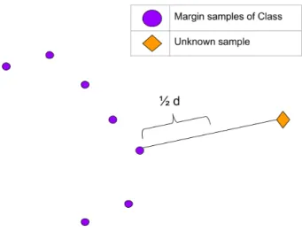
The whole method is based on this stimation, it provides the probability that a sample belongs to a class. This probability will be lower as it gets closer to a margin limit by which the class is defined. This margin limit is equal to half the distance to the closest sample that does not belong to the class, as shown in figure 2.9. As a consequence, it has to be noted that this margin is dependant of the pair of points with which is calculated, so there is there potential margins under different sampling.

Figure 2.9: Margin limit calculation

The way to calculate the probability that x’ is included in the boundary estimated by xi is: Ψ(xi, x0;ki, λi) = exp −   kxi−x0k λi   ki

Having this, the probability that point x’ is associated with class Cl is:

ˆ

(25)

And finally the classification decision is given by:

y∗=

argmaxl∈{1,...,M}Pˆ(Cl|x0) if Pˆ(Cl|x0 ≥δ

’unknown’ Otherwise

Where δ is the threshold on the probability to define the boundary between the known classes and the unsupported open space. This threshold is calculated with cross validation.

2.2.3.5 Model reduction

The number of points used by EVM to represent a class is a reduced subset of the total of points present for this class. Redundant samples can be discarded with little effect on the performance of the classifier. The samples to select are calculated by a minimisation problem. Something important to take into account is that new classes and new samples can affect previously learned models, as it might change the margins that were already calculated.

(26)

CHAPTER 3

METHODOLOGY

In this section we will take a look at how the project was developed. We will explain which technologies, programming languages, frameworks, architectures and data were used and why these choices were taken. First, we are starting with framework and language.

3.1

PyTorch

This project was implemented on PyTorch [17], a Machine Learning framework for Python that is based on Torch and primarily developed by Facebook. It was first released on October 2016 and although it is not currently one of the most used, it is one that is rapidly gaining users at the moment thanks to its simplicity and how easy it is to start without loosing flexibility compared to more complicated frameworks. In figure 3.1 we can see the Google search for Keras, PyTorch and Tensorflow and how Keras and Tensorflow are the most popular at the moment but PyTorch is gaining popularity.

The versions used for this project are Python 2.7 and PyTorch 0.4.1 to be more precise. Now we will have a look at why PyTorch was chosen instead of the other frameworks available for Machine Learning.

3.1.1

Reasons for choosing PyTorch

The main alternatives we considered were Keras with a Tensorflow back-end and PyTorch. We finally chose PyTorch due to the number of advantages we found in respect to Keras and Tensorflow:

(27)

Figure 3.1: Google Search trends for Keras, Tensorflow and PyTorch

1. Easy to start with but flexible. We considered both, Keras and PyTorch, due to their simplicity for beginners. But there is one clear advantage of PyTorch over Keras: flexibility. As Keras is built over other libraries like Tensorflow or Caffe, it is not as flexible; you can not define and personalise each of the layers as much as with PyTorch, for example. This is also the reason why PyTorch has been widely used in research since it appeared, because you can customise the network better with it compared to other frameworks.

2. Easier to debug: You can use Python’s debugger with PyTorch, unlike with Keras or Tensorflow.

3. Dynamic graphs: unlike Tensorflow, that uses a static graph, PyTorch uses dy-namic ones; which means your model can change during its execution. With Tensorflow; and therefore, with Keras, you build the model and operate with it, but with PyTorch the model can be changed and built in execution, changing for different batch of samples if necessary.

4. Well documented: the team made tutorials, documentation, etc. Those are very helpful for beginners and they keep adding to them if the users need them. More-over, they answer any doubt you have in the forum.

Nevertheless, PyTorch has some disadvantages too:

(28)

widely used and have many more examples online and a larger community that can help you solve doubts compared to PyTorch.

2. Tensorboard: This is a platform created for Tensorflow that is meant to help you understand what is happening, debug and optimise your network through some visualisation tools. Pytorch has nothing like this, so you need to make the graphs with the information you want and code them yourself.

Taking all of these into consideration, we finally decided to use PyTorch, as we thought the advantages greatly outbalance the disadvantages.

3.2

Baseline network

For our development of OpenMax we used a ResNet50 [3], which is one of the state of the art networks for image classification and is also available pretrained on PyTorch. The accuracy of this network for ImageNet dataset, which is the one we use, is 76.15%. The special characteristic of a ResNet is that it exploits the benefits of very deep networks and solves the problem of the vanishing or exploding gradient by introducing

residual blocks. Due to the inefficiency of backpropagation, when the depth of a network increases considerably accuracy gets stuck at one point and then it starts decreasing [18]. This problem had already been addressed before with normalised initialisation or normalising middle layers [19] [20], but this method proved better results.

To cope with the vanishing gradient problem this model uses residual blocks, where the output of a layer is the input of the next, and is also added to the output of the second layer to make the input of the third (therefore skipping the intermediate layer) as explained before. The schema of this block was shown on figure 2.4 in section 2.1.1.2, where ResNet50 was explained as part of the state of the art. With reusing some of the previous layers’ activations they expected to reduce the impact of the vanishing phenomenon, as the information of layers will now be repeated. In 2015, they won ImageNet detection, ImageNet localisation, COCO detection, and COCO segmentation, with a Top-5 error of 3.57 in the ImageNet classification task.

3.3

Data

One of the things we want to consider is the data we used for this work. We finally only did object classification but we used a face database to add the different ratios of unknowns to the object one.

(29)

3.3.1

ImageNet

This is one of the most used datasets for image classification, as it is the one provided for the ILSVRC. It was first presented in 2009 in the Conference on Computer Vision and Pattern Recognition (CVPR) and it follows the WordNet hierarchy for ordering the categories of objects. There are a total of 1,281,167 images for training, 50,000 for validation and 100,000 for testing. It has a total of 1,000 categories that make between 732 and 1300 images per category for training, 50 images for each category for validation and 100 per category for testing. This data can be used for non-commercial research and educational purposes only.

We used ImageNet for both, the OpenMax development and for trying EVM.

3.3.2

MSRA-CFW

This is the dataset we used for adding the unknown class. We thought this would be the easier way to get images belonging to a unknown class, as there is no people in the object database. It is Microsoft’s compilation of celebrity faces in the web [21]. It includes a total of 202,792 images of the faces of 1,583 people. It is divided by identity only, so it is up to you to further divide it in training, validation and testing sets. It is publicly available for non-commercial use (research, personal use, academic purpose...) and widely used for face recognition.

3.4

OpenMax implementation

Let us describe the OpenMax method a little bit more on depth in this section. OpenMax is the alternative to SoftMax developed by Abhijit Bendale and Terrance E. Boult for the 2016 CVPRconference [6]. The way this new classifier works is that it recalculates the probability of an image belonging to all classes used during training, but including the option of it being of an unknown class. It does not force all of the probabilities of the categories to add to one, as SoftMax did, however, it is based on this classifier as it also uses probabilities. The steps we have to apply using this method are as follows:

We first need to take all samples in training to extract the features and guess their label as we normally do with any classification task. After this, we take all the samples that the system correctly guessed and we compute aMean Activatin Vector (MAV), which is essentially, a vector with the mean values of the activations of the feature vector of each sample of the class. We will have one MAV per known class,

(30)

that describes the average sample of that class. With this, we can now map all the classes to a feature space and take this MAV as the centroid of each of the classes. Having this information, it is very simple to recognise those samples that are near the mean values of the class as belonging to it, but the challenge appears when we have to categorise those samples that are further away from it. For deciding if an image is part of a class but deviates from the mean or if it is actually an image of an unknown class we will use a Weibull model.

3.4.1

Weibull Model description

A Weibull model is a statistical model based on the Weibull distribution, that is used for analysing and calculating the distribution of unexpected failure in a system. The Probability Desity Function(PDF) of a random sample is:

f(x, λ, k) = ( k λ x λ k−1 e−(x/λ)k if x≥ 0 0 if x < 0

Where k > 0 is the shape parameter and λ > 0 is the scale parameter of the distribution. In this distribution, if k < 1, the failure rate decreases over time; for k = 1 the failure rate is constant in time; and for k > 1, failure rate increases over time. In figure 3.2 we can see how this translates into the shape of the PDF.

This distribution has plenty more uses; such asExtreme Value Theory (EVT), survival analysis, meteorology, insurance... In our case, we use it for EVT. This is a theory employed to analyse the deviations in respect to the expected value. It is commonly used to predict, and analyse the probability of unusually strong floodings, earthquakes and tsunamis, financial risks, structural engineering, etc. So as we can see, it is useful for us as we want to distinguish between samples that belong to a known class but have a high deviation from the mean value and those that do not belong to any of the classes that the network has previously seen.

3.4.2

Calculating the new probabilities

As we want to analyse this extreme values, we take the training samples that are the furthest from the mean, choosing how many of them we take to build the model. To build this model we used the libMR library [22]. With this, we do a High fitting of the unlikely training samples of each class and with this fitting we calculate the probability of the current testing sample of being of each class. For this we need to calculate the distance from the sample to the mean value of the class.

(31)

Figure 3.2: Weibull distribution PDF for different values of k

In SoftMax, we have the following formula for calculating the probabilities: P(y=j|x) = e

vj(x)

PN

i=1evi(x)

As the denominator suggests, the sum of the probabilities is forced to equal 1, and this is exactly what we want to eliminate. For OpenMax, we have the following algorithm 1:

We require v(x), ρj = (µi, λi, ki), µj and α. Where v(x) is the Activation Vector,

µj are the means, ρj are the weibull models and α are the top classes we need to

revise. To calculate the weibul models we needλ, the scale parameter and k, the shape parameter.

With this, we recalculate all probabilities for OpenMax using the CDF of the Weibull distribution (line 3) on the disrance between x and µi. This µi is the MAV of

(32)

Algorithm 1 OpenMax probability estimation 1: Let s(i)argsort(vj(x)); ωj = 1 2: for i= 1, ...,α do 3: ωs(i)(x) = 1− α_α−ie − kx−µs(i)k λs(i) !ks₍_i₎ 4: end for

5: Revise activation vector ˆv(x) =v(x)◦ω(x)

6: Define vˆ0(x) =P_ivi(x)(1−ωi(x)) 7: Pˆ(y=j|x) = e ˆ vj(x) PN i=0eˆvj(x) 8: Let y∗ =argmaxjP(y=j|x 9: Reject input if y∗ == 0 orP(y=y∗|x)<

this computation. Parametersα and the weibull tail size are calibrated in this process too, so that the F-measure and accuracy of OpenMax are optimal.

(33)

CHAPTER 4

RESULTS

In this section we will analyse the results we obtained from this project. As we wanted to improve the results of the traditional SoftMax when including images be-longing to unknown classes, we will compare both methods with this one. For both methods we run 3 different tests with different ratios of known-to-unknown classes in the total datasets. First, we will evaluate our baseline results, the ones obtained with SoftMax.

4.1

SoftMax

As our base-line system we will use SoftMax. Fortesting it we will employ a ResNet50 pretrained on imagenet that is available from PyTorch [23].

Known Unknown Total Accuracy Known Accuracy F-Measure 90% 10% 69.66% 76.01% 81.37% 50% 50% 37.62% 76.01% 54.67% 27% 73% 20.59% 76.01% 34.05%

Table 4.1: Accuracy for SoftMax with different known to unknown ratios Now, we can analyse the results we have for SoftMax on table 4.1. Each row represents a test with a different known-to-unknown ratio. The percentages shown are for the number of images in each category that are mean to show what happens if the majority of images are known, if the majority are unknown or if we have roughly the same number for both. As we expected, SoftMax accuracy proportionally decreases as the amount of unknown images increases due to the lack of ability to deal with new

(34)

classes. The known accuracy, which is the one we have for the known classes (known accuracy) in SoftMax is 76.01%, very close to the accuracy reported by the paper, which is 77.15% [3]. We also calculated the F-Measure because the original paper [6] they reported their results with this measure so that results were less affected by the amount of unknown images that are correctly classified in case of a large number of unknown samples. We have a F-measure that is above the accuracy for all cases, but it still decreases with the number of unknown images. To be consistent with the paper, we define True Positive as the correctly classified samples from the known classes, False positives as the incorrectly guessed from the known classes and False Negatives as the unknown images that were categorised as a known class.

4.2

OpenMax

We can now take a look at how OpenMax does on the same scenarios and if it improved the total accuracy. We should keep in mind that there is not supposed to be a huge difference in the accuracy for only the images that belong to known classes.

First, we can study the configuration of the network and some of the variables of OpenMax. Once again, we used the pretrained ResNet50 that is available in Torchvi-sion, but in this case we needed to extract, not only the results, but the features of the images. The features are taken from the layer just before the last fully connected, which in this case is an average pooling.

For OpenMax we need to calculate the distance from our sample to the MAV making use of euclidean distance, cosine similarity and a sum of both that the authors called eucos distance. In our case, we concluded thatcosine similaritywas giving the best results for all the ratios we tried. In fact, the use of eucos and euclidean distance was giving us the same results with OpenMax as the base results of SoftMax, so no improvement at all.

Finally, for the Weibull distribution we also need the Weibull tail size, which is the number of samples with the furthest distance that we will take into account to do the Weibull fitting of a certain class. The last value we can adjust is the alpha rank. This is a value present in the OpenMax recalculation of probabilities and it is the number of classes we take into consideration from SoftMax that had the highest probability. We finally concluded that the optimal values were 20 for the Weibull tail size and

13 for the Alpha rank.

Looking at the table 4.2 for the results, we can see that the total accuracy improved significantly comparing to SoftMax. The higher the percentage of unknown images, the bigger the improvement. The accuracy of the known classes is reduced around 6%,

(35)

Known Unknown Total Accuracy Known Accuracy F-Measure 90% 10% 72.02% 70.03% 79.07% 50% 50% 50.81% 70.03% 59.16% 27% 73% 39.77% 70.03% 45.28%

Table 4.2: Accuracy for OpenMax with different known to unknown ratios

but the total accuracy improves 13% for the 50-50 configuration and up to almost 20% for the one with a majority of unknown classes. We can also conclude, if we know our testing data will have a considerable number of samples belonging to unknown classes, it is worth to use this alternative instead of SoftMax. As for the F-measure, here is where we can see exactly when OpenMax is more useful. The results of OpenMax are better by a huge difference when the number of unknown images is greater that the known ones, but when the number is more or less even, it only does slightly better that SoftMax. We also see, that if we have many more known images than unknown ones, SoftMax results are slightly better.

To have a better understanding of which images were being misclassified, we also looked at the amount of samples that belonged to a known class and were being clas-sified as unknown (False Unknown), the images that were unknown but were being assigned a preexisting class (False Known), and the number of images that were from one known class and were being incorrectly labeled as another known class (Error). So, we can see this measures for OpenMax in the table 4.3 bellow. Error rates are not included in the table because they were kept very similar to those of the SoftMax, that had a 24% over all known classes. The false negative rate is quite low, which interests us as we did minimise error on the known classes compared with SoftMax. In the case of false positives, in SoftMax it is as high as the percentage of unknown classes, and of course, as we now deal with unknown classes, this number is reduced.

Known Unknown False unknown False known

90% 10% 6.72% 6.4%

50% 50% 4.14% 33.02%

27% 73% 2.27% 51.51%

(36)

4.3

EVM tests

After implementing OpenMax we wanted to compare the method to EVM, as it is the other approach for neural networks to deal with open sets. We tried testing the implementation by another student in the department, but as some of the results and parameters greatly depend on the dataset, we were not able to get concluding results in the amount of time we had. Using his direct implementation in our database, the system always guessed the same class as the label.

(37)

CHAPTER 5

CONCLUSIONS AND FUTURE WORK

5.1

Conclusions

For the thesis, we have implemented a system that is able to classify objects while being able to deal with images of unknown categories. Comparing the results obtained from OpenMax and SoftMax (we can take as example the 50-50 case), we have both a better accuracy and for F-measure. The accuracy is 13% better and the F-measure, as it is not as affected by the correctly guessed unknowns, we have a smaller improvement of 4.5%. We can say that the main goal that we had starting this thesis was achieved, we showed the efficiency of OpenMax as a classifier for open sets.

However, we must note that even if OpenMax results are better for the cases with a higher percentage of unknowns, in the case where 90% of the images belonged to known classes only the accuracy improved and F-measure is better for SoftMax. In cases more similar to this one, we must asses if OpenMax adjusts better to our situation. This will depend on what is more important to the specific case, being able to label known images more accurately or being able to discriminate the images from unknown classes, as the accuracy over the known data decreases by 6%.

In general we can say that open set classification techniques are a powerful and needed tool in certain areas. Some tasks are more benefited than others; for example, these techniques could be specially useful in security for detecting people. Moreover, they could be used to detect errors in datasets and be able to discriminate images that should not be there from the beginning.

All in all, OpenMax opens the way to use neural networks as a classification tech-nique for certain tasks where dealing with open datasets is necessary.

(38)

5.2

Future work

We can improve the results we have for unknown images, as about half of them are being mislabeled as one of the known classes. Based on the idea presented on WSVM, we could try to characterise the class with two models instead of one. Having a model of samples that belong to the class, and another of those that do not belong to it will probably help us define the space and the margins of the classes better. We think that having a better understanding of the samples that do not belong to the class will help to understand the space outside the class and, therefore, help with classification of unknowns.

(39)

BIBLIOGRAPHY

[1] “A Comprehensive Guide to Convolutional Neural Networks.”

[2] O. Russakovsky, J. Deng, H. Su, J. Krause, S. Satheesh, S. Ma, Z. Huang, A. Karpathy, A. Khosla, M. Bernstein, A. C. Berg, and L. Fei-Fei, “ImageNet Large Scale Visual

Recognition Challenge,” International Journal of Computer Vision, vol. 115, pp. 211–

252, 9 2015.

[3] K. He, X. Zhang, S. Ren, and J. Sun, “Deep Residual Learning for Image Recognition,” 2016 IEEE Conference on Computer Vision and Pattern Recognition (CVPR), 2015. [4] W. J. Scheirer and T. E. Boult, “Statistical Methods for Open Set Recognition,” 2016. [5] P. R. M. Júnior, T. E. Boult, J. Wainer, and A. Rocha, “Specialized Support Vector

Machines for open-set recognition,” CoRR, 2016.

[6] A. Bendale and T. Boult, “Towards Open Set Deep Networks,” 2016 IEEE Conference

on Computer Vision and Pattern Recognition (CVPR), 2016. [7] A. Bendale and T. Boult, “OSDN,” 2016.

[8] E. M. Rudd, L. P. Jain, W. J. Scheirer, and T. E. Boult, “The Extreme Value Machine,” IEEE Transactions on Pattern Analysis and Machine Intelligence, 2018.

[9] D. E. King, “Dlib-ml: A Machine Learning Toolkit,” Journal of Machine Learning

Re-search, vol. 10, pp. 1755–1758, 2009.

[10] K. Simonyan and A. Zisserman, “VERY DEEP CONVOLUTIONAL NETWORKS FOR

LARGE-SCALE IMAGE RECOGNITION,” CoR, vol. abs/1409.1556, 2015.

[11] I. Goodfellow, Y. Bengio, and A. Courville,Deep Learning. MIT Press, 2016.

[12] A. Krizhevsky, I. Sutskever, and G. E. Hinton, “ImageNet Classification with Deep

Con-volutional Neural Networks,” inProceedings of the 25th International Conference on

Neu-ral Information Processing Systems - Volume 1, (Lake Tahoe, Nevada), pp. 1097–1105, Curran Associates Inc., 2012.

[13] W. Weibull,A statistical theory of the strength of materials. Stockholm: Generalstabens

litografiska anstalts foÌrlag, 1939.

(40)

[15] W. J. Scheirer, L. P. Jain, and T. E. Boult, “Probability models for open set recognition,” IEEE Transactions on Pattern Analysis and Machine Intelligence, 2014.

[16] A. Bendale and T. Boult, “Towards Open World Recognition,” in Proceedings of the

IEEE Computer Society Conference on Computer Vision and Pattern Recognition, 2015. [17] A. Paszke, S. Gross, S. Chintala, G. Chanan, E. Yang, Z. DeVito, Z. Lin, A. Desmaison,

L. Antiga, and A. Lerer, “Automatic differentiation in PyTorch,” in NIPS-W, 2017.

[18] R. K. Srivastava, K. Greff, and J. Schmidhuber, “Highway Networks,” 5 2015. [19] L. LeCun Yann

}and Bottou, O. G. B., and M. K. Robert, “Efficient BackProp,” in Neural Networks:

Tricks of the Trade (K.-R. Orr Genevieve B.

}and Müller, ed.), pp. 9–50, Berlin, Heidelberg: Springer Berlin Heidelberg, 1998. [20] S. Ioffe and C. Szegedy, “Batch Normalization: Accelerating Deep Network Training by

Reducing Internal Covariate Shift,” inICML, 2 2015.

[21] X. Zhang, L. Zhang, X.-J. Wang, and H.-Y. Shum, “Finding Celebrities in Billions of

Web Images,” IEEE Transactions on Multimedia, vol. 14, pp. 995–1007, 8 2012.

[22] Vision and Security Technology Lab, “Vastlab/libMR: Library for Meta-Recognition and Weibull based calibration of SVM data..”