econstor
Der Open-Access-Publikationsserver der ZBW – Leibniz-Informationszentrum Wirtschaft
The Open Access Publication Server of the ZBW – Leibniz Information Centre for Economics
Nutzungsbedingungen:
Die ZBW räumt Ihnen als Nutzerin/Nutzer das unentgeltliche, räumlich unbeschränkte und zeitlich auf die Dauer des Schutzrechts beschränkte einfache Recht ein, das ausgewählte Werk im Rahmen der unter
→ http://www.econstor.eu/dspace/Nutzungsbedingungen nachzulesenden vollständigen Nutzungsbedingungen zu vervielfältigen, mit denen die Nutzerin/der Nutzer sich durch die erste Nutzung einverstanden erklärt.
Terms of use:
The ZBW grants you, the user, the non-exclusive right to use the selected work free of charge, territorially unrestricted and within the time limit of the term of the property rights according to the terms specified at
→ http://www.econstor.eu/dspace/Nutzungsbedingungen By the first use of the selected work the user agrees and declares to comply with these terms of use.
Christmann, Andreas; Steinwart, Ingo
Working Paper
On robustness properties of convex
risk minimization methods for pattern
recognition
Technical Report // Universität Dortmund, SFB 475 Komplexitätsreduktion in Multivariaten Datenstrukturen, No. 2003,15
Provided in cooperation with:
Technische Universität Dortmund
Suggested citation: Christmann, Andreas; Steinwart, Ingo (2003) : On robustness properties of convex risk minimization methods for pattern recognition, Technical Report // Universität Dortmund, SFB 475 Komplexitätsreduktion in Multivariaten Datenstrukturen, No. 2003,15, http:// hdl.handle.net/10419/49356
Andreas Christmann [email protected]
University of Dortmund Department of Statistics 44221 Dortmund, GERMANY
Ingo Steinwart [email protected]
Modeling, Algorithms and Informatics Group, CCS-3 Mail Stop B256
Los Alamos National Laboratory Los Alamos, NM 87545, USA
Abstract
The paper brings together methods from two disciplines: machine learning theory and robust statistics. Robustness properties of machine learning methods based on convex risk minimization are investigated for the problem of pattern recognition. Assumptions are given for the existence of the influence function of the classifiers and for bounds of the influence function. Kernel logistic regression, support vector machines, least squares and the AdaBoost loss function are treated as special cases. A sensitivity analysis of the support vector machine is given.
Keywords: AdaBoost loss function, influence function, kernel logistic regression, robust-ness, sensitivity curve, statistical learning, support vector machine, total variation
1. Introduction
In pattern recognition and statistical machine learning two major goals are the estimation of a functional relationship y ≈ f(x) between an outcome y and a vector of explanatory variables x = (x1, . . . , xk) ∈Rd and the prediction of an unobserved outcome ynew based
on an observed valuexnew. The functionf is unknown. One needs the implicit assumption
that the relationship between xnew and ynew is − at least almost − the same than in the
training data set (xi, yi), i = 1, . . . , n. Otherwise, it is useless to extract knowledge on
f from the training data set. The classical assumption in machine learning is, that the training data (x, y) are independent and identically generated from an underlying unknown distributionP for a pair of random variables (X, Y). In practical applications the training data set is often quite large, high dimensional and complex. The quality of the predictor
f(x) is measured by some loss function L(y, f(x)). The goal is to find a predictor fP(x) which minimizes the expected loss, i.e.
EPL(Y, fP(X)) = min
f EPL(Y, f(X)). (1)
In this paper we are interested in binary classification, where y ∈ Y := {−1,+1}. The straightforward prediction rule is: predicty= +1 iff(x)≥0, and predicty=−1 otherwise.
The loss function for the classification error is given byI(y, f(x)) =I(yf(x)<0) +I(f(x) = 0)I(y =−1), whereI denotes the indicator function. Inspired by the law of large numbers one might estimatefP by the minimizerfemp of the empirical classification error, that is
femp= arg min f 1 n n i=1 I(yi, f(xi)). (2)
To avoid overfitting one usually has to restrict the class of functions f considered in (2). Unfortunately, the classification functionI is not convex and the minimization of (2) is often NP-hard, cf. Hoeffgen et al. (1995). To circumvent this problem, one minimizes a convex upper bound of the classification error function I(y, f), cf. Sch¨olkopf and Smola (2002) and Vapnik (1998). If L : Y ×R → R is an appropriate convex function, one considers the (approximate) minimization of the empirical risks. Consider the following estimation problems: ˆ fn,λ= arg min f∈Hλf 2 H + 1 n n i=1 L(yi, f(xi)), (3) ( ˆfn,λ,ˆbn,λ) = arg min f∈H, b∈Rλf 2 H+ 1 n n i=1 L(yi, f(xi) +b), (4)
where λ > 0 is a small regularization parameter, H is a reproducing kernel Hilbert space (RKHS) of a kernel k, and b is an unknown real-valued offset. The decision functions are sign( ˆfn,λ) or sign( ˆfn,λ+ ˆbn,λ). Note, that in practice usually (4) is solved while many
theo-retical papers deal with (3) since the unregularized offsetboften causes technical difficulties. Problems (3) and (4) can be interpreted as a stochastic approximation of the minimization of the theoretical regularized risk given in (5) or (6), respectively (cf. Vapnik, 1998, Zhang, 2001; Steinwart, 2002b): fP,λ= arg min f∈Hλf 2 H+EPL(Y, f(X)) (5) (fP,λ, bP,λ) = arg min f∈H, b∈Rλf 2 H +EPL(Y, f(X) +b). (6)
The objective functions in (5) and (6) are denoted by RregL,P,λ(.) and RL,regP,λ(., .) in the fol-lowing. Popular loss functions depend ony and f via v=yf(x) orv=y(f(x) +b). Some important specifications of L are given in Table 1 and plotted in Figure 1. The support vector machine (SVM) penalizes points linearly if v < 1. Kernel logistic regression and AdaBoost use twice continuously differentiable loss functions. The loss function used by kernel logistic regression penalizes misclassifications in a similar way than the SVM, i.e. approximately linearly if v → −∞. The loss function used by AdaBoost increases expo-nentially for v → −∞, cf. Freund and Schapire (1996), Friedman, Hastie and Tibshirani (2000), and Hastie, Tibshirani and Friedman (2001). The modified Huber’s loss function, cf. Zhang (2001), changes the modified least squares loss such that misclassified points with
v <−1 are penalized only linearly.
Steinwart (2002a) shows that SVM’s are universally consistent, i.e. the classification error of ˆfn,λ(.) converges to the optimal Bayes errorEPI(Y, fP(X)) in probability, provided that
Method L L
Kernel Logistic Regression ln(1 + exp(−v)) −1/(1 + exp(v))
AdaBoost exp(−v) −exp(−v)
Support Vector Machine max(1−v,0) sgn(v−1), if v= 1 Modified Huber −4v, ifv <−1 −4, if v <−1
max(1−v,0)2, else −2 max(0,1−v), else
Least Squares (1−v)2 2(v−1)
Modified Least Squares max(1−v,0)2 −2 max(0,1−v) Table 1: Loss functions, v=yf(x).
−3 −2 −1 0 1 2 3
02468
Kernel Logistic Regression
−3 −2 −1 0 1 2 3 02468 AdaBoost −3 −2 −1 0 1 2 3 02468 SVM −3 −2 −1 0 1 2 3 02468 Modified Huber −3 −2 −1 0 1 2 3 02468 Least Squares −3 −2 −1 0 1 2 3 02468
Modified Least Squares
Figure 1: Illustration of different loss functions.
λ = λn tends “slowly” to 0 for n → ∞. Zhang (2001) improves this result by showing
that for many convex loss functions the classifiers based on (3) are universally consistent ifλn→ 0 and λnn→ ∞. Steinwart (2002b) characterizes the loss functions which lead to
universally consistent classifiers and establishes universal consistency for classifiers based on (3) and (4). Furthermore, he shows that there exist solutions of the minimization problems
of the theoretical and of the empirical problems. Moreover, Steinwart (2003) gives lower asymptotical bounds on the number of support vectors, i.e. on the data points with non-vanishing coefficients, and investigates the asymptotic behavior of ˆfn,λ(.) in terms of the
loss function L. Finally, it turns out as a by-product, that the solutions of (3) and (5) are unique. The same holds for the RKHS part of the solutions of (4) and (6). Sch¨olkopf und Smola (2002) describe other support vector machines and give an overview on algorithms to solve the minimization problems corresponding to SVMs.
Obviously, the proof that many classifiers based on convex loss functions are universally consistent under weak conditions is a strong argument in favor of these statistical learning methods. Nevertheless, it is important to investigate robustness properties for such statis-tical learning methods for the following reasons. In practice one has to apply the methods to a data set with a finite sample size. Outliers often occur in real data sets. Outliers can be described as data points which ’are far away. . .from the pattern set by the majority of the data’, see Hampel et al. (1986, p. 25). There are many reasons for the occurrence of outliers, e.g. typing errors and gross errors, which are errors due to a source of deviations which acts only occasionally but is quite powerful. From a robustness point of view the occurrence of outliers is only one of several possible deviations from the assumed model. There are often no or virtually no gross errors in high-quality data, but 1% to 10% of gross errors in routine data seem to be more the rule than the exception, cf. Hampel et al. (1986, p.27f). Especially in large data mining problems the data quality is sometimes far from being optimal, cf. Hipp et al. (2001). Obviously, it isnot the goal tomodel the occurrence of typing errors or gross errors. Goals of robust statistics are to investigate the impact such data points can have on the results of estimation or testing methods and the development of methods such that the impact of such data points is bounded. Main strategies of robust statistics are Huber’s minimax approach (Huber, 1964; Huber, 1981), Hampel’s influence function (Hampel, 1974; Hampel et al., 1986), the finite sample breakdown point proposed by Donoho and Huber (1983), Rieder’s approach based on least favourable local alterna-tives (Rieder, 1994), and the regression depth method proposed by Rousseeuw and Hubert (1999).
Here, we will use the approach based on the influence function. This approach can be applied to quite general models and the influence function has a nice interpretation. A method is called robust in the theory of robust statistics based on influence functions, if the method is based on a functional with a bounded influence function. From the viewpoint of robust statistics it is therefore important to investigate the impact a small amount of contamination of the ’true’ probability measureP can have on the statistical learning pro-cess which is specified via the functionals defined by RregL,P,λ(.) andRregL,P,λ(., .). Hence, this paper investigates robustness properties of statistical learning methods based on convex risk minimization.
The rest of the paper is organized as follows. Section 2 gives the definitions of the influence function and the sensitivity curve, which are the two robustness concepts we are dealing with. Section 3 and Section 4 contain the main results. In Section 3 sufficient conditions are given for the existence of the influence function for classifiers based on (5) and (6). In Section 4 it is shown that the influence function of the functional in (6) and the difference quotient used in the definition of the influence function for (5) can be bounded independently ofzandP. Section 5 describes the results of some simulation experiments to
gain insight into the robustness properties of the SVM for finite sample sizes and investigates the impact a single data point can have if a radial basis function kernel or a linear kernel is used. Section 6 contains the conclusion. Finally, the Appendix gives the proofs of the main theorems discussed in this paper.
2. Influence function and sensitivity curve
Goals of robust statistics are the investigation of robustness properties of statistical methods and the development of methods with good robustness properties. One major approach of robust statistics is the influence function of functionals proposed by Hampel (1974) and Hampel et al. (1986). Here, a map T which assigns to every distribution P on a given set Z an element T(P) of a given Banach space E is called a functional. In the case of the convex risk minimization methods (5) and (6) E equals the RKHS and T(P) =fP,λ or
T(P) = (fP,λ, bP,λ), respectively.
Definition 1 Influence function. The influence function of a functional T at a point z for a distribution P is the special Gˆateaux derivative (if existent)
IF(z;T,P) = lim ε↓0 T(1−ε)P+εΔz −T(P) ε , (7)
where Δz is the Dirac distribution at the point z.
The influence function has the interpretation, that it measures the impact of an (infinites-imal) small amount of contamination of the original distributionP in direction of a Dirac distribution located in the pointz on the theoretical quantity of interest T(P). Therefore, in the robustness approach based on influence functions it is desirable that a statistical method is based on a functional with a bounded influence function.
The sensitivity curve SCn proposed by J.W. Tukey (cf. Hampel et al., 1986, p. 93) can
be interpreted as a finite sample version of the influence function (see (9)). The sensitivity curve measures the impact of just one additional data pointz on the empirical quantity of interest, i.e. on the estimateTn.
Definition 2 Sensitivity curve. The sensitivity curve of an estimator Tn at a pointzgiven
a data set z1, . . . , zn−1 is defined by
SCn(z;Tn) =n
Tn(z1, . . . , zn−1, z)−Tn−1(z1, . . . , zn−1)
. (8) If the estimator Tn is defined via a functional T(Pn), where Pn denotes the empirical
distribution of the data points z1, . . . , zn, then it holds forεn= 1/n:
SCn(z;Tn) = T(1−εn)Pn−1+εnΔz −T(Pn−1) εn . (9)
For many estimators the sensitivity curve converges to the influence function, as ntends to infinity. Counterexamples are given e.g. in Davies (1993).
3. Existence of the influence function
In this section we give sufficient conditions for the existence of the influence function for classifiers based on (5) and (6). Throughout this sectionBE denotes the closed unit ball of
a Banach space E. We first recall a simplified version of the implicit function theorem in Banach spaces (cf. Akerkar, 1999; Zeidler, 1986):
Theorem 3 LetE, F be Banach spaces andG:E×F →F be a continuously differentiable map. Suppose that we have (x0, y0) ∈ E ×F such that G(x0, y0) = 0 and ∂G∂F(x0, y0) is
invertible. Then there exists aδ >0 and a continuously differentiable mapf :x0+δBE →
y0+δBF such that for all x∈x0+δBE, y∈y0+δBF we have
G(x, y) = 0 if and only if y=f(x).
Moreover, the derivative off is given by
f(x) =− ∂G ∂F x, f(x) −1 ∂G ∂E x, f(x).
For the application of the implicit function theorem we have to show that certain operators are invertible. For this the following theorem which is known as the Fredholm Alternative (cf. Cheney, 2001) turns out to be helpful:
Theorem 4 LetE be a Banach space andK:E →Ebe a compact operator. ThenidE+K
is surjective if and only if it is injective.
We first establish a result for classifiers based on (5) with smooth loss function:
Theorem 5 Let L:Y ×R→[0,∞) be a convex and twice continuously differentiable loss function. Furthermore, let X⊂Rd be compact, H be a RKHS of a continuous kernel onX
and P be a distribution on X×Y. Then the influence function of the classifiers based on (5) exists for all z∈X×Y.
Remark 6 By a simple modification of the proof of the above theorem we actually find that the special Gˆateaux derivative ofT :P→fP,λ exists for every direction, i.e.
lim
ε↓0
f(1−ε)P+ε˜P,λ−fP,λ
ε
exists for all distributions P and P˜ on X×Y provided that the assumptions of Theorem 5 hold. This is an interesting result from the view of applied statistics, because a point mass contamination is just one possible kind of contamination which can occur in practice.
The following theorem shows the existence of the influence function for classifiers based on (6):
Theorem 7 Let L:Y ×R→[0,∞) be a convex and twice continuously differentiable loss function with L>0. Furthermore, let X⊂Rdbe compact, H be a RKHS of a continuous
kernel onX andPbe a distribution onX×Y. Then the influence function of the classifiers based on (6) exists for all z∈X×Y.
Remark 8 As in the case of problem (5) a slight modification of the proof gives that T :
P→(fP,λ, bP,λ) is special Gˆateaux differentiable.
Remark 9 Considering the loss functions in Table 1 we immediately see that the above theorems apply to the kernel logistic regression, the least squares and the AdaBoost loss function. The second derivatives of the modified least squares and the modified Huber loss function fail to exists in only one point. For the loss function of the standard SVM, even the first derivative does not exist in one point.
4. Bounds on the influence function
As mentioned in Section 2, a desirable property of a robust statistical method is that its corresponding functional has a bounded influence function. In this section we show that for certain loss functions the influence function can be bounded independently of z and P for classifiers based on (5) and (6). For the formulation of our results we need to recall that the norm of total variation of a signed measure μon a spaceX is defined by
μM :=|μ|(X) := sup n i=1 |μ(Ai)|:A1, . . . , An is a partition ofX .
For more information on this norm we refer to Brown and Pearcy (1977).
Our first result bounds the difference quotient in the definition of the influence function for classifiers based on (5). In particular, it states that the influence function of these classifiers is uniformly bounded whenever it exists. Please note, that the following theorem based on Steinwart (2002b) applies to all six loss functions given in Table 1 because differentiability of Lis not assumed. Furthermore, this theorem shows that the sensitivity curves of all six methods are uniformly bounded if we setε= 1/n, see (9).
Theorem 10 Let L :Y ×R→[0,∞) be a continuous and convex loss function. Further-more, let X⊂Rd be compact and H be a RKHS of a continuous kernel onX. Then for all
λ >0there exists a constant cL(λ)>0explicitly given in (20) such that for all distributions P and P˜ onX×Y we have f(1−ε)P+εP˜,λ−fP,λ ε H ≤cL(λ) P−P˜M, ε >0.
Unfortunately, using the estimate of Steinwart (2002b) does not give any meaningful result for classifiers based on (6). Therefore, the approach of the following theorem is to apply the formula for the derivative given by the implicit function theorem.
Theorem 11 LetL:Y ×R→[0,∞) be a convex and twice continuously differentiable loss function with a≤L ≤b for some a, b >0. Furthermore, letX ⊂Rd be compact, H be a
RKHS of a continuous kernel on X and Tλ(P) = (fP,λ, bP,λ) be given by (6). Then for all
λ >0 there exists a constant cL(λ)>0 such that for all distributions P on X×Y and all
z∈X×Y we have
Remark 12 Theorem 11 applies to (6) with the least squares loss function. However, Theorem 11 covers neither the logistic regression function as we only have L ≥0 nor the AdaBoost loss function which satisfies L=L= exp(−.) However, we get the same bound of the influence function if we restrict our considerations to distributions Pwith
a ≤
L(Y, fP,λ(X) +bP,λ)dP ≤ b (10)
for some b≥a >0. A simple sufficient condition for the latter can be derived by the proof of Steinwart (2002b, Lemma II.6): let Aρy := {x ∈ X : P(y|x) > ρ}, y ∈ Y, ρ > 0, and
αP(ρ) :=ρmin{PX(A ρ
1),PX(A ρ
−1)}. Fixingλ >0, a twice continuously differentiableLand
a threshold α >0 there exists b≥a >0 such that everyP with αP(ρ)≥α for some ρ >0
satisfies (10). Note, that the assumption αP(ρ) ≥ α guarantees that the two classes of P are “balanced”.
Remark 13 As mentioned in Remark 8 the map T : P → (fP,λ, bP,λ) is special Gˆateaux
differentiable. A simple modification of the proof of Theorem 11 shows that the special Gˆateaux derivative ofT can be uniformly bounded.
Remark 14 Consider the case thatPandP˜ are probability measures with densitiespandp˜
with respect to some dominating measure ν. Then, the last two theorems also give bounds of the influence functions in terms of the Hellinger metricH(P,P˜) = [(√p−√p˜)2dν]1/2. This
follows from a relationship between the norm of total variation and the Hellinger metric:
P−P˜M ≤2H(P,˜P)≤2P−P˜1/2 M .
5. Empirical results for the SVM
In this section we study the impact an additional data point can have on the SVM with offsetbfor pattern recognition. An analogous investigation for the case without offset gave similar results to those described in this section. We generated a training data set with
n= 500 data pointsxi from a bivariate normal distribution with expectationμ= (0,0) and
covariance matrix Σ. The variances were set to 1, whereas the covariance was set to 0.5. The responsesyiwere generated from a classical logistic regression model withθ= (−1,1),
b= 0.5, such thatP(Yi= +1) = [1 + exp(−(xiθ+b))]−
1 andP(Y
i=−1) = 1−P(Yi = +1).
The computations were done using the software SVMlight developed by Joachims (1999). SVMlight solves the dual program corresponding to the primal optimization problem
arg minf∈H, b∈R 2Cn1 ||f||2H + 1 n n i=1 ξi such that yi(f(xi) +b)≥1−ξi ξi ≥0. (11)
We consider two popular kernels: a Gaussian radial basis function (RBF) kernelf(x, x) = exp(−γx −x2) and a linear kernel. Appropriate values for γ and for the constant
C (or λ) are important for the SVM and are often determined by cross validation, cf. Sch¨olkopf and Smola (2002, p. 217). A cross validation based on the leave-one-out er-ror for the training data set was carried out by a two-dimensional grid search on γ ∈
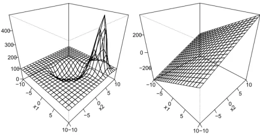
x1 −10 −5 0 5 10 x2 −10 −5 0 5 10 0 100 200 300 400 x1 −10 −5 0 5 10 x2 −10 −5 0 5 10 −200 0 200
Figure 2: Sensitivity function of ˆf+ˆb, if the additional data pointzis located atz= (x, y), wherex= (6,6) and y= 1. Left: RBF kernel. Right: linear kernel.
{0.05,0.1,0.25,0.5,0.75,1,1.5,2,3,4,5,10,20} and C ∈ {0.5,0.75,1,1.25, 1.5,1.75,2,5,10,
20}. As a result of the cross validation, the tuning parameters for the SVM with RBF kernel were set toγ = 0.25 and C = 2. The leave-one-out error for the SVM with a linear kernel turned out to be stable over a broad range of values for C. We usedC = 1 in the computations for the linear kernel. For n = 500 this results in λ= (2Cn)−1 = 5×10⁻⁴
for the RFB kernel and λ= (2Cn)−1 = 0.001 for the linear kernel. Please note, that such
small values ofλwill result in relatively large bounds.
Figure 2 shows the sensitivity curves of ˆf+ˆb:= ˆfn,λ+ˆb, if we add a single pointz= (x, y)
to the original data set, where x1 = 6, x2 = 6, and y= +1. The additional data point has
a local and smooth impact on ˆf + ˆb with a peak in a neighorhood of (x1, x2), if one uses
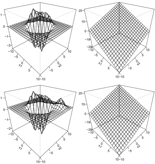
the RBF kernel. For a linear kernel, the impact is approximately linear. The reason for this different behavior of the SVM with different kernels becomes clear from Figure 3 where plots of ˆf+ˆbare given for the original data set and for the modified data set, which contains the additional data point z. Please note, that the RBF kernel yields ˆf + ˆb approximately equal to zero outside a central region, as almost all data points are lying inside the central region. Comparing the plots of ˆf+ˆbbased on the RBF kernel for the modified data set with the corresponding plot for the original data set, it is obvious that the additional smooth peak is due to the new data point located atx= (6,6) withy = 1. It is interesting to note, that although the estimated functions ˆf + ˆb for the original data set and for the modified data set based on the SVM with the linear kernel are looking quite similar, the sensitivity curve is similar to an affine hyperplane which is affected by the value ofz. This allows the interpretation, that just a single data point can have an impact on ˆf + ˆb estimated by a SVM with a linear kernel over a broader region than for an SVM with an RBF kernel.
Now, we study the impact of an additional data point z = (x, y), where y = 1, on the percent of classification errors and on the fittedy−value forz. We vary zover a grid in the
x1 −10 −5 0 5 10 x2 −10 −5 0 5 10 −2 −1 0 1 x1 −10 −5 0 5 10 x2 −10 −5 0 5 10 −20 −10 0 10 20 x1 −10 −5 0 5 10 x2 −10 −5 0 5 10 −2 −1 0 1 x1 −10 −5 0 5 10 x2 −10 −5 0 5 10 −20 −10 0 10 20
Figure 3: Plot of ˆf + ˆb. Upper left: RBF kernel, original data set. Upper right: linear kernel, original data set. Lower left: RFB kernel, modified data set. Lower right: linear kernel, modified data set. The modified data set contains the additional data pointz= (x, y), where x= (6,6) and y= 1.
x−coordinates. Figure 4 shows that the percentage of classification errors is approximately constant outside the central region that contains almost all data points if a Gaussian RBF kernel was used. For the SVM with a linear kernel, the percentage of classification errors tends to be approximately constant in one halfspace but changes in the other halfspace. The response of the additional data point was correctly estimated by ˆy= +1 outside the central region, if a RBF kernel is used, see Figure 5. In contrast to that, using a linear kernel results in estimated responses ˆy = +1 or ˆy = −1 of the additional data point depending on the affine halfspace in which thex−value ofz is lying. Finally, let us study the impact of an additional data point located atz= (x, y), wherey= 1, on the estimated parameters ˆband ˆ
x1 −10 −5 0 5 10 x2 −10 −5 0 5 10 28.0 28.5 29.0 x1 −10 −5 0 5 10 x2 −10 −5 0 5 10 29.2 29.4 29.6 29.8 30.0 30.2
Figure 4: Percent of classification errors if one data pointz= (x,1) is added to the original data set, wherex varies over the grid. Left: RBF kernel. Right: linear kernel
x1 −10 −5 0 5 10 x2 −10 −5 0 5 10 −1.0 −0.5 0.0 0.5 1.0 x1 −10 −5 0 5 10 x2 −10 −5 0 5 10 −1.0 −0.5 0.0 0.5 1.0
Figure 5: Fitted y−value for new observation if one data point z = (x,1) is added to the original data set, where x varies over the grid. Left: RBF kernel. Right: linear kernel
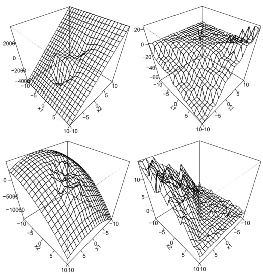
As the plots for ˆθ1 and ˆθ2 are looking very similar, we only show the latter. Please note,
that the axes are not identically in Figure 6 due to the kernels. The sensitivity curves for the slopes estimated by the SVM with an RBF kernel are similar to a hyperplane outside the central region, which contains almost all data points. In the central region, there is a smooth transition between regions with higher sensitivity values and regions with lower sensitivity values. The sensitivity curves for the slopes of the SVM with a linear kernel are flat in one affine halfspace, but change approximately linear in the other affine halfspace. This behavior also occurs for the sensitivity curve of the offset by using a linear kernel.
x1 −10 −5 0 5 10 x2 −10 −5 0 5 10 −4000 −2000 0 2000 x1 −10 −5 0 5 10 x2 −10 −5 0 5 10 −60 −40 −20 0 20 x1 −10 −5 0 5 10 x2 −10 −5 0 5 10 −10000 −5000 0 x1 −10 −5 0 5 10 x2 −10 −5 0 5 10 0 5 10
Figure 6: Sensitivity function for ˆθ and ˆb, respectively. Upper left: Sensitivity function for ˆ
θ2, RBF kernel. Upper right: Sensitivity function for ˆθ2, linear kernel. Lower
left: Sensitivity function for ˆb, RBF kernel. Lower right: Sensitivity function for ˆb, linear kernel.
In contrast to that, the sensitivity curve of the offset based on a SVM with a RBF kernel shows a smooth but curved shape outside the region containing the majority of the data points.
6. Concluding remarks
In this paper, we used the influence function approach of robust statistics (Hampel et al., 1986) for recent statistical learning methods based on convex risk minimization methods for the problem of pattern recognition. Special cases of such convex risk minimization methods are the support vector machine, kernel logistic regression, AdaBoost, and least squares. Assumptions were derived for the existence of the influence function of the classifiers and also
for bounds of the influence function which hold uniformally with respect to the distribution
P and the pointz of the Dirac distribution Δz describing the contamination. For the case
without offsetbone can uniformly bound the difference quotient considered by the influence function under weak conditions which also yields uniform bounds for Tukey’s sensitivity curve. In particular, the influence function for these classifiers is uniformly bounded if it exists. Some of the results are not limited to the special Gˆateaux derivative used in the definition of the influence function. The assumptions of some of our results exclude the support vector machine because the SVM uses a loss function which is not differentiable in one point. Hence, we gave some numerical results for the sensitivity curve, which can be interpreted as a final sample version of the influence function, of the SVM classifier. It turned out, that the popular exponential radial basis function kernel resulted in smooth sensitivity curves for ˆf + ˆb and for the estimated coefficients (ˆθ,ˆb). Varying the position of one additional data point had a smooth and local impact on ˆf+ ˆb, if one uses an RBF kernel. For the linear kernel the impact of varying one additional data point behaves also in a relatively smooth manner, but the impact seems to be more globally than locally.
We briefly like to mention that the sensitivity curves for the slope parameters of a support vector machine with a RBF kernel k(x, x) = exp(−γx−x2) are looking quite similar to
rotated sensitivity curves or to influence functions of robust S-estimators based on a smooth
ρ−function in the linear regression model. This might be a consequence of a relationship be-tween the SVM using a RBF kernel and robust S-estimators based on a smoothρ−function fulfilling the usual properties (cf. Davies, 1990): (a)ρ(u) =ρ(−u),u∈R, (b)ρ(u),u >0, is nonincreasing, continuous at 0 and continuous on the left, and (c) for somec >0,ρ(u)>0 if|u| ≤c, and ρ(u) = 0 if |u|> c, which is true e.g. for ρc(u) =
1−u2/c22, if |u|<=c,
ρc(u) = 0 else. The RBF kernel k of a SVM considered as a function of u=x−x has
similar properties than theρ−function used by S-estimators. Consider the linear regression model yi = xiθ+εi, 1 ≤ i ≤n, where yi ∈ R, xi ∈ Rp, and θ ∈ Rp. Further, assume εi,
1≤i≤n, are independently and identically distributed random variables with respect to some distribution P such that P(εi ≤ u) = F(u/σ), u ∈ R, where σ ∈ (0,∞) is a scale
parameter andF :R→[0,1] is a nondegenerate distribution function. An S-estimate (ˆθ,σˆ) of (θ, σ) is implicitly defined by minimizing a scale parameter σ subject to an inequality constraint, i.e. arg minθ∈Rp, σ∈(0,∞) σ (12) s.t. n1ni=1 ρ yi−xiθ σ ≥1−ε, (13)
cf. Rousseeuw and Yohai (1984) and Davies (1990). The constraint guarantees that at leastn(1−ε) of the residuals (yi−xiθ)/σ have absolute values less than of equal toc due
to property (c) of the ρ−function. Formula (11) allows the interpretation that the SVM minimizes an average plus a regularized squared norm (and hence a measure for variability) with respect to several inequality constraints.
For a numerical comparison between the support vector machine and the regression depth method recently proposed by Rousseeuw and Hubert (1999) see Christmann and Rousseeuw (2001) and Christmann, Fischer and Joachims (2002).
It would be interesting to study the influence function of convex risk minimization meth-ods for other problems, e.g. ε−regression or kernel principal component analysis, or to
con-sider other robustness concepts proposed by Huber (1981) and Donoho and Huber (1983), but this is beyond the scope of this paper.
Acknowledgments
The financial support of the Deutsche Forschungsgemeinschaft (SFB 475, ”Reduction of complexity in multivariate data structures”) is gratefully acknowledged.
Appendix A.
In this appendix we prove the theorems from Section 3 and Section 4.
Proof of Theorem 5. Let Φ :X →Hbe the feature map ofH, i.e. Φ(x) :=k(x, .),
wherek is the kernel ofH. Let us consider the map G:R×H→H that is defined by
G(ε, f) := 2λf+E(1−ε)P+εΔzL(Y, f(X))Φ(X).
Note, that the above expectation is actually a Bochner integral in H. Furthermore, for
ε ∈ [0,1] the expectation is with respect to a signed measure. Obviously, forε∈ [0,1] we obtain G(ε, f) = ∂R reg L,(1−ε)P+εΔz,λ ∂H (f). Since RregL,(1−ε)P+εΔ
z,λ is convex for all ε ∈ [0,1] we have G(ε, f) = 0 if and only if f =
f(1−ε)P+εΔz,λ for such ε. Our aim is to show the existence of a differentiable function
ε→ fε defined on a small interval [−δ, δ] for some δ >0 that satisfies G(ε, fε) = 0 for all
ε∈[−δ, δ]. Once we have shown the existence of this function we immediately obtain
IF(z;T,P) = ∂fε
∂ε (0).
For the existence ofε→fεwe only have to check by Theorem 3 thatGis continuously
differ-entiable and that ∂H∂G(0, fP,λ) is invertible. Let us start with the first: an easy computation
shows
∂G
∂ε(ε, f) =−EPL
(Y, f(X))Φ(X) +E
ΔzL(Y, f(X))Φ(X). (14)
Moreover, using the reproducing propertyΦ(x), g=g(x), g∈H, x∈X we find
∂G
∂H(ε, f) = 2λidH +E(1−ε)P+εΔzL
(Y, f(X))Φ(X), .Φ(X). (15)
It is a simple routine to check that both partial derivatives are continuous. This together with the continuity ofG ensures that Gis continuously differentiable (cf. Akerkar, 1999). In order to show that∂H∂G(0, fP,λ) is invertible it suffices to show by the Fredholm Alternative
that ∂H∂G(0, fP,λ) is injective and that
defines a compact operator on H. To show the compactness recall that Φ(X) is compact by the continuity of Φ. Therefore, there exists ac >0 such that
Ag ∈c·aco Φ(X)
for all g ∈ BH. Since the closure of the absolute convex hull aco Φ(X) is compact the
desired compactness of the operatorA follows. Furthermore, forg= 0 we find (2λidH +A)g,(2λidH +A)g = 4λ2g, g+ 4λg, Ag+Ag, Ag > g,EPL(Y, fP,λ(X))g(X)Φ(X) = EPL(Y, fP,λ(X))g2(X) ≥ 0
since the second derivative of a convex function is always nonnegative. Therefore, ∂G∂H(0, fP,λ) =
2λidH +A is injective.
Proof of Theorem 7. We sometimes write L(f+b) instead of L(Y, f(X) +b) to
shorten the notation, if misunderstandings are unlikely. We use this kind of notation also for derivatives of L. The proof is similar to that of Theorem 5. However, due to the extra variableb we have to modify our approach: we define the mapG:R×H×R→H×Rby
G(ε, f, b) :=
2λf+E(1−ε)P+εΔzL(f +b)Φ,E(1−ε)P+εΔzL(f+b)
.
Again, forε∈[0,1] the definition of Gensures
G(ε, f, b) =
∂RregL,(1−ε)P+εΔ
z,λ
∂(H×R) (f) ,
if we apply the identification (H×R) = H×R. Since RregL,(1−ε)P+εΔ
z,λ is convex for all
ε∈[0,1] we haveG(ε, f, b) = 0 if and only if (f, b) minimizesRL,reg(1−ε)P+εΔ
z,λfor suchε. Our
aim is to apply the implicit function theorem in the way we did it in the proof of Theorem 5. However, this time the implicit function theorem will also ensure the uniqueness of the solution of (6). Obviously, this is necessary for the existence of the influence function. In order to apply Theorem 3 we need the partial derivatives ofG. By an easy computation we find ∂G ∂ε(ε, f, b) =−EPL (Y, f(X) +b)Φ(X) +E ΔzL(Y, f(X) +b)Φ(X) and ∂G ∂(H×R)(ε, f, b) = 2λidH +EεL(f +b)Φ, .Φ EεL(f +b)Φ EεL(f+b)Φ EεL(f +b) ,
where we use the abbreviation Eε:=E(1−ε)P+εΔz. A routine check shows that bothG and
the partial derivatives are continuous and henceGis continuously differentiable.
Now, let us fix a solution (fP,λ, bP,λ) of (6). Existence of a solution follows from Zhang
∂G
∂(H×R)(0, fP,λ, bP,λ) is invertible it suffices to show by the Fredholm Alternative that ∂G
∂(H×R)(0, fP,λ, bP,λ) is injective and that
K:= EPL(fP,λ+bP,λ)Φ, .Φ EPL(fP,λ+bP,λ)Φ EPL(fP,λ+bP,λ)Φ EPL(fP,λ+bP,λ)−2λ ,
is a compact operator on H×R. The latter can be seen using the argument of the proof of Theorem 5. For the former let us suppose that we have an element (g, t) ∈H×Rwith (2λidH×R+K)(g, t) = 0. This is equivalent to the following linear system of equations
2λg+EPL(fP,λ+bP,λ)gΦ +tEPL(fP,λ+bP,λ)Φ = 0 (16) EPL(fP,λ+bP,λ)g+tEPL(fP,λ+bP,λ) = 0. (17)
Let us first assume thatt= 0. Then the above system yields 2λg+EPL(fP,λ+bP,λ)gΦ = 0.
Using the techniques of the proof of Theorem 5 we easily find that this implies g = 0. Therefore, we may assume without loss of generality that t = 1. In order to avoid long notations we introduce the measure μ := L(fP,λ +bP,λ)dP. Note, that L > 0 implies
μ= 0. Now, (17) yields
μ(g) =−μ(1), (18) where1 denotes the constant function with value 1. Hence, by (16) we find
0 = 2λg, g+μ(g2) +μ(g) = 2λg, g+μ(g2)−μ(1). (19) Furthermore, (18) implies
0≤μ((g+1)2) =μ(g2) + 2μ(g) +μ(1) =μ(g2)−μ(1).
This together with (19) yields 2λg, g ≤0 and henceg= 0. However, the latter contradicts (18) and hence there is no non-trivial solution of the system (16), (17).
Now, the implicit function theorem states in particular, that the solution (fP,λ, bP,λ) is
unique in a small neighborhood of (fP,λ, bP,λ). Hence it is globally unique since the set of
solutions of (6) is convex. The rest of the proof follows the ideas of the proof of Theorem 5.
Proof of Theorem 10. Recall that every convex function onR is locally Lipschitz
continuous. Let |L|Y×[−c,c]|1 denote the Lipschitz constant of L restricted to Y ×[−c, c],
c > 0. We define δλ :=
(L(−1,0) +L(1,0))/λ and K := supx∈Xk(x, x). We fix a distribution P. An easy estimate (cf. Steinwart, 2002b) shows fP,λ∞ ≤δλK. Now, by
Theorem 3.15 in Steinwart (2003) there exists a measurable functionh :X×Y → Rwith h∞≤L|Y×[−δλK,δλK]1 such that for all distributions ˆPwe have
fP,λ−fPˆ,λH ≤
1
where Φ :X → H is the feature map of H. Now let ˆP:= (1−ε)P+εP˜. Then the above inequality yields ε−1f(1−ε)P+ε˜P,λ−fP,λH ≤ (ελ)−1EPhΦ−E(1−ε)P+ε˜PhΦH = λ−1EPhΦ−E˜PhΦH ≤ cL(λ)P−˜PM, where cL(λ) =λ−1KL|Y×[−δλK,δλK]1. (20)
This shows the assertion.
Proof of Theorem 11. By rescaling problem (6) we may assume without loss of
generality that K:= supx∈Xk(x, x)≤1. Recall, that in the proof of Theorem 7 we used
IF(z;T,P) = ∂(fε, bε)
∂ε (0),
where ε → (fε, bε) was the function implicitly defined by G(ε, f, b) = 0. The implicit
function theorem hence gives
IF(z;T,P) =−S−1◦∂G
∂ε(0, fP,λ, bP,λ) , (21)
whereS := ∂(H∂G×R)(0, fP,λ, bP,λ). Therefore, it suffices to bound the norms of the operators
on the right side of (21). We begin with
∂G∂ε(0, fP,λ, bP,λ)
= EPL(fP,λ+bP,λ)Φ−EΔzL(fP,λ+bP,λ)Φ
≤ bP−ΔzM.
Furthermore, for (g, t)∈H×Rwe have
S(g, t) = 2λidH +EPL(fP,λ+bP,λ)Φ, .Φ EPL(fP,λ+bP,λ)Φ EPL(fP,λ+bP,λ)Φ EPL(fP,λ+bP,λ) g t = 2λg+EPL(fP,λ+bP,λ)gΦ +tEPL(fP,λ+bP,λ)Φ EPL(fP,λ+bP,λ)g+tEPL(fP,λ+bP,λ) .
As in the proof of Theorem 7 we write μ:=L(fP,λ+bP,λ)dP. Then we find
S(g, t),(g, t)= 2λg, g+μ(g2) + 2tμ(g) +t2μ(1). (22) Let us suppose that (g, t)= 1. Then there existw∈H withw= 1 and s∈[0,1] such that g=sw and t=±√1−s2. Note, that since K ≤1 we have |μ(w)| ≤μ(1). Therefore,
(22) yields S(g, t),(g, t) ≥ 2λs2−2s1−s2μ(1) + (1−s2 )μ(1) ≥ 2λs2−2s(1−s)μ(1) + (1−s2)μ(1) = 2λs2+s2μ(1)−2sμ(1) +μ(1) ≥ λμ(1) 2λ+μ(1),
where the last estimate is based on a simple minimization with respect tos. By the proof of Pedersen (1989, Prop. 3.2.12) we hence find
S(g, t) ≥ λμ(1)
2λ+μ(1)(g, t) for all (g, t)∈H×R. Hence we obtain
S−1 ≤ λμ(1) 2λ+μ(1) −1 = 1 λ+ 2 μ(1) . Since L≥aimplies μ(1)≥a >0 we have shown the assertion.
References
Akerkar, R. Nonlinear Functional Analysis. Narosa Publishing House, New Dehli, 1999. Brown, A. and Pearcy, C. Introduction to Operator Theory I. Springer, New York, 1977. Cheney, W. Analysis for Applied Mathematics. Springer, New York, 2001.
Christmann, A., Fischer, P. and Joachims, T. Comparison between various regression depth methods and the support vector machine to approximate the minimum number of mis-classifications. Computational Statistics, 17:273-287, 2002.
Christmann, A. and Rousseeuw, P.J. Measuring overlap in logistic regression.Computational Statistics and Data Analysis, 37:65-75, 2001.
Davies, P.L. The asymptotics of S-estimators in the linear regression model. Ann. Statist., 18:1651-1675, 1990.
Davies, P.L. Aspects of robust linear regression.Ann. Statist., 21:1843-1899, 1993.
Donoho, D.L. and Huber, P.J. (1983). The Notion of Breakdown Point. InA Festschrift for Erich L. Lehmann, eds. P.J. Bickel, K.A. Doksum, and J.L. Hodges, Jr., pages 157-184, Belmont, California, Wadsworth, 1983.
Friedman, J., Hastie, T. and Tibshirani, R. Additive logistic regression: a statistical view of boosting (with discussion). Ann. Statist., 28:337-407, 2000.
Freund, Y. and Schapire, R. Experiments with a new boosting algorithm. In: Machine Learning: Proceedings of the 13th International Conference, pages 148-156, Morgan Kauffman, San Francisco, 1996.
Hampel, F.R. The influence curve and its role in robust estimation.J. Amer. Statist. Assoc., 69:383-393, 1974.
Hampel, F.R., Ronchetti, E.M., Rousseeuw, P.J., Stahel, W.A.Robust statistics: The Ap-proach Based on Influence Functions. Wiley, New York, 1986.
Hastie, T., Tibshirani, R. and Friedman, J. The Elements of Statistical Learning. Data Mining, Inference and Prediction. Springer, New York, 2001.
Hipp, J., G¨untzer, Grimmer, U. (2001). Data Quality Mining - Making a Virtue of Ne-cessity. Workshop on Research Issues in Data Mining and Knowledge Discovery DMKD. Santa Barbara, CA. Available electronically athttp://www.cs.cornell.edu/johannes/ papers/dmkd2001-papers/p5_hipp.pdf
H¨offgen, K.U., Simon, H.-U. and van Horn, K.S. Robust Trainability of Single Neurons.
J. Computer and System Sciences, 50:114-125, 1995.
Huber, P.J. Robust estimation of a location parameter. Ann. Math. Statist., 35:73-101, 1964.
Huber, P.J.Robust Statistics.Wiley, New York, 1981.
Joachims, T.Making large-Scale SVM Learning Practical. InAdvances in Kernel Methods -Support Vector Learning, eds: B. Sch¨olkopf, C. Burges, A. Smola. MIT Press, Cambridge, Massachusetts, 1999.
Pedersen, G.K. Analysis Now. Springer, New York, 1989.
Rieder, H. Robust Asymptotic Statistics. Springer, New York, 1994.
Rousseeuw, P.J. and Yohai, V. Robust regression by means of S-estimators. Robust and Nonlinear Time Series Analysis. Lecture Notes in Statist., 26:256-272, 1984.
Rousseeuw, P.J. and Hubert, M. Regression Depth. J. Amer. Statist. Assoc., 94:388-433, 1999.
Sch¨olkopf, B. and Smola, A.J. Learning with Kernels. Support Vector Machines, Regular-ization, OptimRegular-ization, and Beyond. MIT Press, Cambridge, Massachusetts, 2002.
Steinwart, I. Support vector machines are universally consistent.J. Complexity, 18:768-791, 2002a.
Steinwart, I. Consistency of support vector machines and other regularized kernel machine. Preprint. Available electronically at http://www.c3.lanl.gov/~ingo/publications/ info-02.ps, 2002b.
Steinwart, I. Sparseness of support vector machines. Preprint. Available electronically at
http://www.c3.lanl.gov/~ingo/publications/jmlr-03.ps, 2003.
Vapnik, V. Statistical Learning Theory, Wiley, New York, 1998.
Zeidler, E.Nonlinear Functional Analysis and its Applications I, Springer, New York, 1986. Zhang, T. Statistical behaviour and consistency of classification methods based on convex