Unified processing framework of high-dimensional and overly imbalanced chemical datasets for virtual screening.

(1)

PhD Thesis

Unified Processing Framework of

High-Dimensional and Overly Imbalanced

Chemical Datasets for Virtual Screening

Author:

Amir Ali Rafati Afshar

Supervisors:

Dr. Emili Balaguer Ballester

Professor Mark Hadfield

A thesis submitted in partial fulfilment of the requirements of

Bournemouth University for the degree of Doctor of Philosophy

(2)

(3)

I

Copyright Statement

This copy of the thesis has been supplied on condition that anyone who consults it is understood to recognise that its copyright rests with the author and due acknowledgement must always be made of the use of any material contained in, or derived from, this thesis.

(4)

II

Abstract

Virtual screening in drug discovery involves processing large datasets containing unknown molecules in order to find the ones that are likely to have the desired effects on a biological target, typically a protein receptor or an enzyme. Molecules are thereby classified into active or non-active in relation to the target. Misclassification of molecules in cases such as drug discovery and medical diagnosis is costly, both in time and finances. In the process of discovering a drug, it is mainly the inactive molecules classified as active towards the biological target i.e. false positives that cause a delay in the progress and high late-stage attrition. However, despite the pool of techniques available, the selection of the suitable approach in each situation is still a major challenge.

This PhD thesis is designed to develop a pioneering framework which enables the analysis of the virtual screening of chemical compounds datasets in a wide range of settings in a unified fashion. The proposed method provides a better understanding of the dynamics of innovatively combining data processing and classification methods in order to screen massive, potentially high dimensional and overly imbalanced datasets more efficiently.

(5)

III

List of Figures

Figure 1: Compound attrition and cost increase of drug discovery process by time

(Bleicher et al. 2003, p.371) ... 3

Figure 2: A graph with nodes (a, b and c) and edges (lines that connect the nodes ab, ac and bc) ... 7

Figure 3: A Hydrogen-depleted molecular graph of Caffeine (Brown, 2009) ... 7

Figure 4: Connection table example with an example molecule ... 8

Figure 5: Example of a line formula for the molecule shown in Figure 4. ... 9

Figure 6: SMILES, IUAPC and InCHi representations for Caffeine (Source: Brown 2009) ... 10

Figure 7: Example of Structure-key fingerprint (Brown 2009) ... 17

Figure 8: Pseudocode of a typical Hash-key fingerprint (Brown 2005) ... 18

Figure 9: The structuring on a Hash-Key fingerprint (Brown 2009) ... 19

Figure 10: Example of two fingerprints and the similarity and distance coefficient calculated. ... 22

Figure 11: Iterative process during HTS between various research groups (Stephan & Gilbertson 2009) ... 23

Figure 12: Showing the key factors towards a successful HTS process (Stephan & Gilbertson 2009) ... 24

Figure 13: A schematic illustration of a typical virtual screening flowchart (Leach & Gillet 2007) ... 26

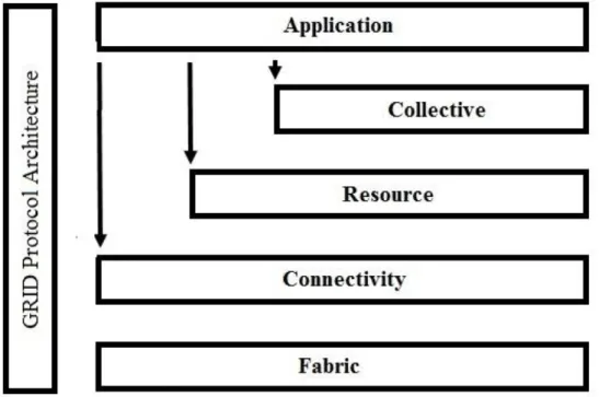
Figure 14: Typical Grid protocol computing architecture (Foster et al. 2008) ... 28

Figure 15: Typical Cloud computing architecture (Foster et al. 2008) ... 30

Figure 16: Schematic overview of chapter 3... 39

(8)

VI Figure 18: Illustrating how the introduction of noise can affect the learning

classifier’s ability to learn decision boundaries. (Source Weiss 2004) ... 50

Figure 19: Generating synthetic samples by SMOTE... 54

Figure 20: An example of how to calculate non-repeating combinations for a group of 7 fingerprints ... 74

Figure 21: Classification results from classifying the Bursi dataset by J48. ... 79

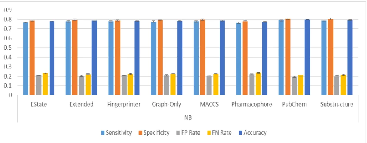
Figure 22: Classification results from classifying the Bursi dataset by Naïve Bayes. ... 80

Figure 23: Classification results from classifying the Bursi dataset by Random Forest. ... 80

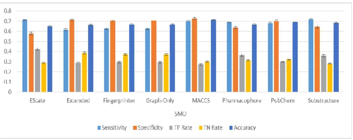
Figure 24: Classification results from classifying the Bursi dataset by SMO. ... 81

Figure 25: Classification results from classifying the Bursi dataset by Majority Voting. ... 81

Figure 26: Results from adding numerical fingerprints to binary fingerprints for J48 ... 82

Figure 27: Results from adding numerical fingerprints to binary fingerprints for Naïve Bayes ... 83

Figure 28: Results from adding numerical fingerprints to binary fingerprints for Random Forest ... 83

Figure 29: Results from adding numerical fingerprints to binary fingerprints for SMO ... 83

Figure 30: Results from adding numerical fingerprints to binary fingerprints for Majority Voting ... 83

Figure 31: Classifier performance for EState– Original ... 84

Figure 32: Classifier performance for MACCS– Original ... 84

Figure 33: Classifier performance for Pharmacophore– Original... 85

Figure 34: Classifier performance for PubChem– Original ... 85

(9)

VII Figure 36: Results from adding numerical fingerprints to binary fingerprints for EState ... 86 Figure 37: Results from adding numerical fingerprints to binary fingerprints for

MACCS ... 86 Figure 38: Results from adding numerical fingerprints to binary fingerprints for

Pharmacophore ... 86 Figure 39: Results from adding numerical fingerprints to binary fingerprints for

PubChem ... 86 Figure 40: Results from adding numerical fingerprints to binary fingerprints for

Substructure ... 86 Figure 41: Classification results from classifying the Bursi dataset by J48 – PCA ... 87 Figure 42: Classification results from classifying the Bursi dataset by Naïve Bayes –

PCA ... 87 Figure 43: Classification results from classifying the Bursi dataset by Random Forest

– PCA ... 88 Figure 44: Classification results from classifying the Bursi dataset by SMO – PCA 88 Figure 45: Classification results from classifying the Bursi dataset by Majority

Voting – PCA ... 88 Figure 46: Results from adding numerical fingerprints to binary fingerprints for J48 ... 89 Figure 47: Results from adding numerical fingerprints to binary fingerprints for

NaïveBayes ... 90 Figure 48: Results from adding numerical fingerprints to binary fingerprints for

Random Forest ... 90 Figure 49: Results from adding numerical fingerprints to binary fingerprints for

SMO ... 90 Figure 50: Results from adding numerical fingerprints to binary fingerprints for

Majority Voting ... 90 Figure 51: Classifier performance for EState – PCA ... 91

(10)

VIII

Figure 52: Classifier performance for MACCS – PCA ... 91

Figure 53: Classifier performance for Pharmacophore – PCA ... 92

Figure 54: Classifier performance for PubChem – PCA Applied... 92

Figure 55: Classifier performance for Substructure – PCA Applied ... 92

Figure 56: Results from adding numerical fingerprints to binary fingerprints for EState – PCA ... 93

Figure 57: Results from adding numerical fingerprints to binary fingerprints for MACCS – PCA ... 93

Figure 58: Results from adding numerical fingerprints to binary fingerprints for Pharmacophore – PCA ... 93

Figure 59: Results from adding numerical fingerprints to binary fingerprints for PubChem – PCA ... 93

Figure 60: Results from adding numerical fingerprints to binary fingerprints for Substructure – PCA ... 94

Figure 61: Sensitivity versus False Positive rate for the methods used on the Mutagenicity dataset. ... 94

Figure 62: Sensitivity versus False Positive rate per classifier for the Mutagenicity dataset. ... 95

Figure 63: Classification results from classifying the Fontaine dataset by J48 ... 99

Figure 64: Classification results from classifying the Fontaine dataset by NaïveBayes ... 100

Figure 65: Classification results from classifying the Fontaine dataset by Random Forest ... 100

Figure 66: Classification results from classifying the Fontaine dataset by SMO .... 100

Figure 67: Classification results from classifying the Fontaine dataset by Majority Voting ... 101

(11)

IX Figure 69: Results from adding numerical fingerprints to binary fingerprints for

NaïveBayes ... 102

Figure 73: Classifier performance for by EState - Original ... 103

Figure 74: Classifier performance for MAACS - Original ... 103

Figure 75: Classifier performance for Pharmacophore - Original ... 103

Figure 76: Classifier performance for PubChem - Original... 104

Figure 77: Classifier performance for Substructure - Original ... 104

Figure 78: Results from adding numerical fingerprints to binary fingerprints for EState ... 104

Figure 79: Results from adding numerical fingerprints to binary fingerprints for MACCS ... 105

Figure 80: Results from adding numerical fingerprints to binary fingerprints for Pharmacophore ... 105

Figure 81: Results from adding numerical fingerprints to binary fingerprints for PubChem ... 105

Figure 82: Results from adding numerical fingerprints to binary fingerprints for Substructure ... 105

(12)

X Figure 87: Classification results from classifying the Fontaine dataset by Majority Voting ... 107 Figure 88: Results from adding numerical fingerprints to binary fingerprints for J48 ... 107 Figure 89: Results from adding numerical fingerprints to binary fingerprints for

Majority Voting ... 108 Figure 93: Classifier performance for EState – Original SMOTEd All... 109 Figure 94: Classifier performance for MACCS – Original SMOTEd All ... 109 Figure 95: Classifier performance for Pharmacophore – Original SMOTEd All .... 109 Figure 96: Classifier performance for PubChem – Original SMOTEd All ... 110 Figure 97: Classifier performance for Substructure – Original SMOTEd All... 110 Figure 98: Results from adding numerical fingerprints to binary fingerprints for

EState ... 110 Figure 99: Results from adding numerical fingerprints to binary fingerprints for

Substructure ... 111 Figure 103: Classification results from classifying the Fontaine dataset by J48 ... 112

(13)

XI Figure 104: Classification results from classifying the Fontaine dataset by NaïveBayes ... 112 Figure 105: Classification results from classifying the Fontaine dataset by Random

Forest ... 112 Figure 106: Classification results from classifying the Fontaine dataset by SMO .. 112 Figure 107: Classification results from classifying the Fontaine dataset by Majority

Voting ... 113 Figure 108: Results from adding numerical fingerprints to binary fingerprints for J48 ... 113 Figure 109: Results from adding numerical fingerprints to binary fingerprints for

Majority Voting ... 114 Figure 113: Classifier performance for EState – Original SMOTEd Training ... 115 Figure 114: Classifier performance for MACCS – Original SMOTEd Training .... 115 Figure 115: Classifier performance for Pharmacophore – Original SMOTEd Training ... 115 Figure 116: Classifier performance for PubChem – Original SMOTEd Training .. 116 Figure 117: Classifier performance for Substructure – Original SMOTEd Training ... 116 Figure 118: Results from adding numerical fingerprints to binary fingerprints for

(14)

XII Figure 120: Results from adding numerical fingerprints to binary fingerprints for

Pharmacophore ... 117

Figure 122: Results from adding numerical fingerprints to binary fingerprints for Substructure ... 117

Figure 126: Classification results from classifying the Fontaine dataset by SMO . 118 Figure 127: Classification results from classifying the Fontaine dataset by Majority Voting ... 119

Figure 129: Results from adding numerical fingerprints to binary fingerprints for NaïveBayes ... 119

Figure 133: Classifier performance for EState – PCA Dataset ... 121

Figure 134: Classifier performance for MACCS – PCA Dataset ... 121

Figure 135: Classifier performance for Pharmacophore – PCA Dataset ... 121

Figure 136: Classifier performance for PubChem – PCA Dataset ... 122

(15)

XIII Figure 138: Results from adding numerical fingerprints to binary fingerprints for EState ... 122 Figure 139: Results from adding numerical fingerprints to binary fingerprints for

Substructure ... 123 Figure 143: Classification results from classifying the Fontaine dataset by J48 ... 124 Figure 144: Classification results from classifying the Fontaine dataset by

NaïveBayes ... 124 Figure 145: Classification results from classifying the Fontaine dataset by Random

Forest ... 124 Figure 146: Classification results from classifying the Fontaine dataset by SMO .. 124 Figure 147: Classification results from classifying the Fontaine dataset by Majority

Majority Voting ... 126 Figure 153: Classifier performance for EState – PCA SMOTEd All ... 127

(16)

XIV

Figure 154: Classifier performance for MACCS – PCA SMOTEd All ... 127

Figure 155: Classifier performance for Pharmacophore – PCA SMOTEd All ... 127

Figure 156: Classifier performance for PubChem – PCA SMOTEd All ... 128

Figure 157: Classifier performance for Substructure – PCA SMOTEd All ... 128

Figure 161: Classifier performance for PubChem ... 129

Figure 162: Classifier performance for Substructure ... 129

Figure 166: Classification results from classifying the Fontaine dataset by SMO .. 130

Figure 167: Classification results from classifying the Fontaine dataset by Majority Voting ... 131

(17)

XV Figure 172: Results from adding numerical fingerprints to binary fingerprints for Majority Voting ... 132 Figure 173: Classifier performance for EState – PCA SMOTEd Training ... 133 Figure 174: Classifier performance for MACCS – PCA SMOTEd Training ... 133 Figure 175: Classifier performance for Pharmacophore – PCA SMOTEd Training ... 133 Figure 176: Classifier performance for PubChem – PCA SMOTEd Training ... 134 Figure 177: Classifier performance for Substructure – PCA SMOTEd Training .... 134 Figure 178: Results from adding numerical fingerprints to binary fingerprints for

Substructure ... 135 Figure 183: Sensitivity versus False Positive Fontaine methods ... 136 Figure 184: Sensitivity versus False Positive Fontaine classifiers ... 136 Figure 185: Classification results from classifying the AID362 dataset by

NaïveBayes ... 140 Figure 186: Classification results from classifying the AID362 dataset by Random

Forest ... 140 Figure 187: Classification results from classifying the AID362 dataset by Majority

Voting ... 140 Figure 188: Results from adding numerical fingerprints to binary fingerprints for

(18)

XVI Figure 189: Results from adding numerical fingerprints to binary fingerprints for

Majority Voting ... 141

Figure 190: Classifier performance for MACCS – Original ... 141

Figure 191: Classifier performance for Pharmacophore – Original... 142

Figure 192: Classifier performance for PubChem – Original ... 142

Figure 196: Classification results from classifying the AID362 dataset by NaïveBayes ... 144

Figure 197: Classification results from classifying the AID362 dataset by SMO ... 144

Figure 202: Classifier performance for Pharmacophore – Original SMOTEd All .. 146

Figure 203: Classifier performance for PubChem – Original SMOTEd All ... 146

Figure 204: Classifier performance for Substructure – Original SMOTEd All ... 146

(19)

XVII Figure 207: Results from adding numerical fingerprints to binary fingerprints for Substructure ... 147 Figure 208: Classification results from classifying the AID362 dataset by

NaïveBayes ... 148 Figure 209: Classification results from classifying the AID362 dataset by SMO ... 148 Figure 210: Classification results from classifying the AID362 dataset by Majority

SMO ... 149 Figure 214: Classifier performance for Pharmacophore – Original SMOTEd Training ... 150 Figure 215: Classifier performance for PubChem – Original SMOTEd Training .. 150 Figure 216: Classifier performance for Substructure – Original SMOTEd Training ... 150 Figure 217: Results from adding numerical fingerprints to binary fingerprints for

Substructure ... 151 Figure 220: Classification results from classifying the AID362 dataset by

NaïveBayes ... 152 Figure 221: Classification results from classifying the AID362 dataset by SMO ... 152 Figure 222: Results from adding numerical fingerprints to binary fingerprints for

(20)

XVIII Figure 223: Results from adding numerical fingerprints to binary fingerprints for

Majority Voting ... 153

Figure 224: Classifier performance for EState - PCA ... 154

Figure 225: Classifier performance for Pharmacophore - PCA ... 154

Figure 226: Classifier performance for PubChem - PCA ... 154

Figure 229: Classification results from classifying the AID362 dataset by NaïveBayes ... 156

Figure 230: Classification results from classifying the AID362 dataset by SMO ... 156

Figure 235: Classifier performance for PubChem – PCA SMOTEd All ... 158

Figure 236: Classifier performance for Substructure – PCA SMOTEd All ... 158

(21)

XIX Figure 240: Results from adding numerical fingerprints to binary fingerprints for Substructure ... 159 Figure 241: Classification results from classifying the AID362 dataset by

Forest ... 160 Figure 243: Classification results from classifying the AID362 dataset by SMO ... 160 Figure 244: Results from adding numerical fingerprints to binary fingerprints for J48 ... 161 Figure 245: Results from adding numerical fingerprints to binary fingerprints for

Majority Voting ... 161 Figure 247: Classifier performance for MACCS – PCA SMOTEd Training ... 162 Figure 248: Classifier performance for Pharmacophore – PCA SMOTEd Training ... 162 Figure 249: Classifier performance for Substructure – PCA SMOTEd Training .... 162 Figure 250: Results from adding numerical fingerprints to binary fingerprints for

Substructure ... 163 Figure 253: Sensitivity versus False Positive AID362 methods ... 164 Figure 254: Sensitivity versus False Positive AID362 classifiers ... 164 Figure 255: Classification results from classifying the AID456 dataset by

NaïveBayes ... 167 Figure 256: Classification results from classifying the AID456 dataset by SMO ... 167

(22)

XX Figure 257: Results from adding numerical fingerprints to binary fingerprints for NaïveBayes ... 168 Figure 258: Results from adding numerical fingerprints to binary fingerprints for

Random Forest ... 168 Figure 259: Classifier performance for MACCS ... 169 Figure 260: Classifier performance for PubChem ... 169 Figure 261: Classifier performance for Substructure ... 169 Figure 262: Results from adding numerical fingerprints to binary fingerprints for

NaïveBayes ... 171 Figure 266: Classification results from classifying the AID456 dataset by SMO ... 171 Figure 267: Results from adding numerical fingerprints to binary fingerprints for J48 ... 172 Figure 268: Results from adding numerical fingerprints to binary fingerprints for

Majority Voting ... 173 Figure 272: Classifier performance for MACCS ... 173 Figure 273: Classifier performance for PubChem ... 174

(23)

XXI Figure 274: Results from adding numerical fingerprints to binary fingerprints for EState ... 174 Figure 275: Results from adding numerical fingerprints to binary fingerprints for

NaïveBayes ... 175 Figure 278: Classification results from classifying the AID456 dataset by SMO ... 175 Figure 279: Results from adding numerical fingerprints to binary fingerprints for J48 ... 176 Figure 280: Results from adding numerical fingerprints to binary fingerprints for

Majority Voting ... 176 Figure 282: Classifier performance for EState ... 177 Figure 283: Classifier performance for Pharmacophore ... 177 Figure 284: Classifier performance for Substructure ... 178 Figure 285: Results from adding numerical fingerprints to binary fingerprints for

Pharmacophore ... 178 Figure 287: Classification results from classifying the AID456 dataset by

Forest ... 179 Figure 289: Classifier performance for EState ... 180 Figure 290: Classifier performance for Pharmacophore ... 181 Figure 291: Classifier performance for Substructure ... 181

(24)

XXII Figure 292: Results from adding numerical fingerprints to binary fingerprints for EState ... 182 Figure 293: Results from adding numerical fingerprints to binary fingerprints for

NaïveBayes ... 182 Figure 296: Classification results from classifying the AID456 dataset by SMO ... 183 Figure 297: Results from adding numerical fingerprints to binary fingerprints for

Majority Voting ... 184 Figure 300: Classifier performance for MACCS ... 184 Figure 301: Classifier performance for Pharmacophore ... 185 Figure 302: Classifier performance for PubChem ... 185 Figure 303: Results from adding numerical fingerprints to binary fingerprints for

NaïveBayes ... 187 Figure 308: Classification results from classifying the AID456 dataset by SMO ... 187

(25)

XXIII Figure 309: Results from adding numerical fingerprints to binary fingerprints for NaïveBayes ... 187 Figure 310: Results from adding numerical fingerprints to binary fingerprints for

Majority Voting ... 188 Figure 312: Classifier performance for EState ... 189 Figure 313: Classifier performance for MACCS ... 189 Figure 314: Classifier performance for Pharmacophore ... 189 Figure 315: Classifier performance for PubChem ... 190 Figure 316: Classifier performance for Substructure ... 190 Figure 317: Results from adding numerical fingerprints to binary fingerprints for

Substructure ... 191 Figure 320: Sensitivity versus False Positive AID456 methods ... 191 Figure 321: Sensitivity versus False Positive AID456 classifiers ... 192 Figure 322: Bursi dataset classifiers’ performance ... 197 Figure 323: Bursi dataset methods’ performance ... 197 Figure 324: Fontaine dataset methods’ performance ... 198 Figure 325: Fontaine dataset classifiers’ performance... 199 Figure 326: AID362 dataset methods’ performance ... 200 Figure 327: AID362 classifiers’ performance... 200 Figure 328: AID456 methods’ performance ... 201 Figure 329: AID456 classifiers’ performance... 201

(26)

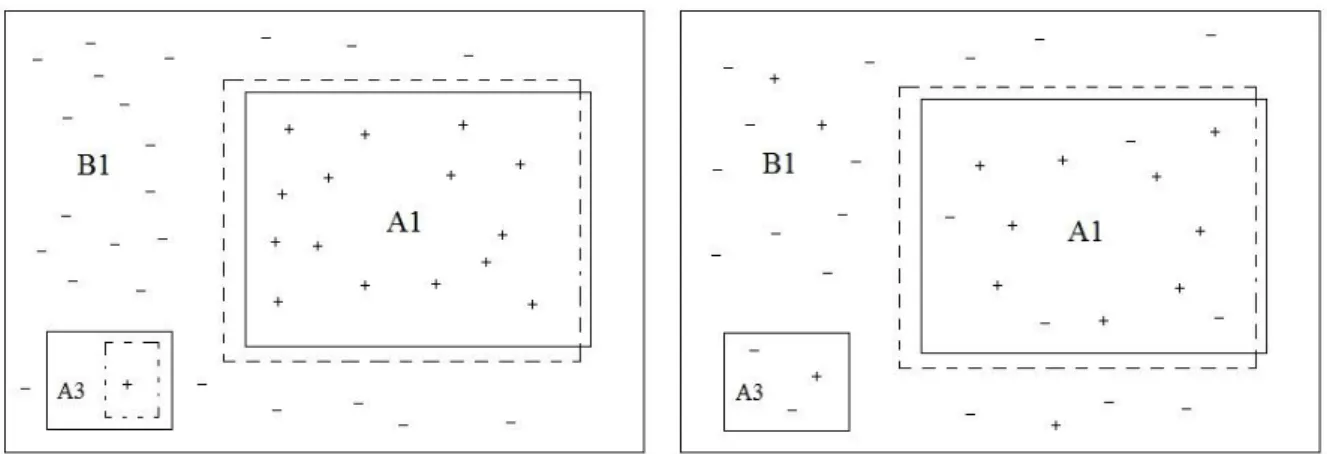
XXIV Figure 330: Possible class imbalance scenarios (Amended from Sáez et al. 2016, p.161) ... 205 Figure 331: Various types of examples identified in a multi-class situation (Sáez et

(27)

XXV

List of Tables

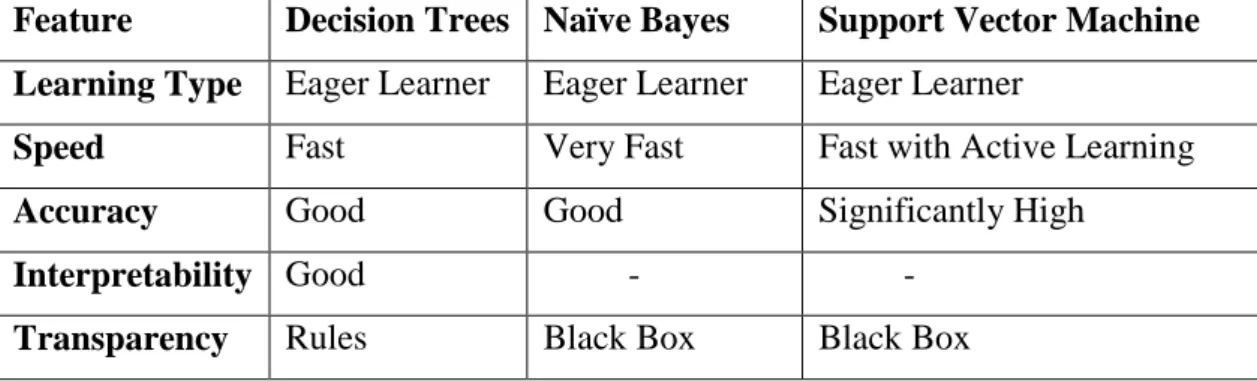
Table 1: AID362 specifications. Class of interest has a 1 next to the label ... 34 Table 2: AID456 specification. Class of interest has a 1 next to its label... 35 Table 3: Mutagenicity dataset specification. ... 35 Table 4: Factor XA dataset specification. ... 36 Table 5: Detailing the properties of the various fingerprints used ... 43 Table 6: Misclassification of raw PubChem datasets #1 ... 51 Table 7: Misclassification of raw PubChem datasets #2 ... 51 Table 8: A cost matrix showing the misclassification cost for positives and negatives ... 52 Table 9: Original number of samples in unbalanced datasets ... 57 Table 10: Number of samples in balanced datasets ... 57 Table 11: Advantages of decision trees, Naïve Bayes, SVM classifiers. (Source:

Galathiya et al. 2012) ... 68 Table 12: Some of the features from classifiers used in this study. (Source: Galathiya

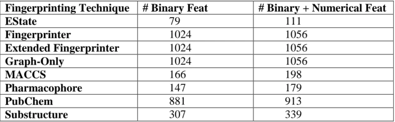
et al. 2012) ... 69 Table 13: Summary of the number of features generated by various fingerprinting

techniques ... 74 Table 14: Mutagenicity dataset specification. Class of interest labelled as 1. ... 78 Table 15: Euclidean distance for the methods used ... 95 Table 16: Euclidean distance for the classifiers used... 95 Table 17: Factor XA dataset specification. Class of interest labelled as 1 ... 98 Table 18: Euclidean distance for the methods used ... 136 Table 19: Euclidean distance for the classifiers used... 137 Table 20: AID362 dataset specification. Class of interest labelled as 1 ... 139

(28)

XXVI Table 21: Euclidean distance for the methods used ... 164 Table 22: Euclidean distance for the classifiers used... 165 Table 23: AID456 Dataset specification. Class of interest labelled as 1 ... 167 Table 24: Euclidean distance for the methods used ... 192 Table 25: Euclidean distance for the classifiers used... 192

(29)

XXVII

Acknowledgements

To Emili: Thank you for being such an amazing supervisor, for your support at times when I needed it most and for believing in me and motivating me.

To Naomi: Thank you for your support in all the stages of this degree. To Mark: Thank you for supporting us with taking this degree further.

To all my friends and colleagues at Bournemouth University: Thank you for being part of this journey and for making it a very pleasant one. Special thanks go to Ed, Manuel, Cristina, Rashid, Anna and Alex.

This work is dedicated to my Mother, who has supported me through all my decisions in life. Without you I would have never been able to get this far in my life. Thank you and God bless you.

To my Father for great advices and good thoughts throughout this journey.

I would like to thank the School of Design, Engineering and Computing, SMART Technology Research Centre and the Graduate School for their help in administration and financial support with expenses. Special thanks to Kelly Duncan Smith, Malcolm Green, Angela Tabeshfar, Pattie Davis and Fiona Knight.

Bournemouth University, thank you for providing a productive and enjoyable research and work environment.

(30)

XXVIII

List of Abbreviations

DM Data Mining

ESt EState Fingerprinter

Ext CDK Extended Fingerprinter Fin CDK Fingerprinter

FNR False Negative Rate FPR False Positive Rate Gra CDK Graph-Only HTS High-Throughput Screening MAC MACCS NB NaïveBayes Pha Pharmacophore Pub PubChem RF Random Forest

SMO Sequential Minimal Optimisation Sub Substructure

TNR True Negative Rate TPR True Positive Rate VS Virtual Screening

(31)

1

1. Introduction

Virtual screening in drug discovery involves screening datasets containing unknown molecules in order to find the ones that are likely to have the desired effects on a biological target. The molecules are thereby classified into active or non-active compared to the target. Misclassification of molecules in cases such as drug discovery and medical diagnosis is costly, both in time and finances. In the process of discovering a drug, it is mainly the inactive molecules classified as active towards the biological target i.e. false positives that cause a delay in the progress and high late-stage attrition.

1.1. Background

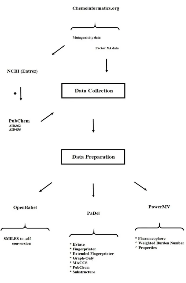
Chemoinformatics (Cheminformatics) as defined by Frank Brown (1998) is the mixing of resources in order to transform data into information and information into knowledge in order to make faster and better decisions in the field of drug identification and optimisation. In short, computational methods are used to process chemical data in particular the chemical data structure. Some of the techniques used in Chemoinformatics such as computational chemistry and QSAR (Quantitative Structure-Activity Relationship) are very well-known and –established and have been practiced for years in the industry and laboratories.

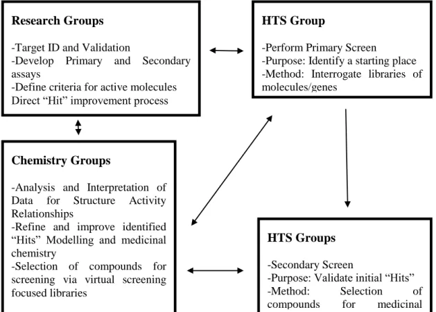
Drug discovery is the process by which new medicinal candidates are discovered. To achieve this, compounds which are likely to have wanted effects on a biological target (disease) are identified and isolated. High-Throughput screening (HTS) is used to assess the binding ability –activity of compounds against the target. This is also known as empirical or physical screening. HTS screens thousands of compounds in order to find new candidates in a fast and accurate manner. There are two stages of screenings: primary and secondary (confirmatory). The biological relevance of the compounds identified as hits from the primary stage are assessed. These compounds are then screened for a second time. Confirmed hits from this stage are called leads which will be further optimised to become candidates for clinical tests. Advances in molecular biology and the use of combinatorial chemistry have resulted in an increase in the number of biological targets and compounds in libraries. HTS is characterised by its screening capacity which is about 10000 –

(32)

2 100000 compounds per day. The significant increase in the number of available compounds as well as biological targets requires scientists to reduce the size of HTS assays (Mayr & Bojanic 2009). Considering the fact that HTS is a very costly process, alternative techniques such as virtual screening could be utilised in order to filter compounds which are selected for screening.

Virtual screening or biophysical screening is the in-silico screening of compounds. It uses computational methods to score, rank or filter a set of compound structures. Virtual screening can be used to determine which compounds to screen against a given target. It has been acknowledged that in order to identify desirable compounds from a library there needs to be an increase in the quality of the library rather than the quantity (Bajorath 2002). This helps carry out fewer but smarter experiments. Virtual screening assists the detection of new bioactive compounds by reducing the number of compounds that are to be screened based on scoring criteria. This reduction is achieved by eliminating the compounds which do not show activity towards a given target.

HTS has become an important source for identifying new compounds for optimisation in medium to large pharmaceuticals. It has proven to be a useful technology for providing new hits for the drug discovery process. However not all hits identified by HTS are appropriate leads for further medicinal optimisations. In fact the overall HTS success rate currently is estimated at 45-55% (S. Fox et al. 2006; Keserü & Makara 2009). HTS suffers from two types if errors: type 1 and type 2 (Martis et al. 2011). Type 1 errors are false positives. These are compounds which are regarded as actives but later turn out to be non-active. Type 2 errors are false negatives. These are active compounds which are regarded as non-actives in the screening process. One of the main challenges in HTS is to differentiate between compounds which are genuinely active towards a target and false positive compounds. In biological terms a compound that is genuinely active against a target has a high tendency to form a non-covalent bond with the target which is reversible (Thorne et al. 2010). All other compounds that form bindings with the target but do not possess the characteristics of the genuine interaction are false positives. These compounds are generally active in an assay, but their activity is target-independent. They can affect by forming aggregates, they can be protein-active or interfere with assay signalling. This all leads to them being considered as active and therefore the

(33)

3 secondary screenings normally include a great deal of false positive compounds. Manually filtering compounds using the knowledge of chemists is a good way of reducing false positives but as mentioned in (Sink et al. 2010) an analysis of such a method showed inconsistency in the compounds which were to be taken out.

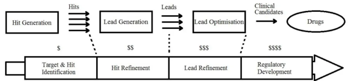
False positive compounds escape various screenings undetected. They are one of reasons there is high late-stage attrition in the drug discovery process. These are compounds which fail to qualify as being suitable lead compounds for drug optimisation. The costs of the process increase as we get to the later stages of it, as seen in Figure 1.

Figure 1: Compound attrition and cost increase of drug discovery process by time(Bleicher et al. 2003, p.371)

It can also be seen in Figure 1 that as we get to the later stages of the process the number of compounds decrease (the number of arrows). There are fewer compounds to work with and the processes become more expensive. For example in the pharmaceutical industry, the main pre-clinical expense is the lead optimisation process (Jorgensen 2012). It makes sense to have more suitable compounds (opportunities) at hand in order to increase the chances of discovering better leads.

1.2. Project description and goals

The main objective of this project is to explore and investigate the application and the effects of using various fingerprinting methods combined with the Synthetic Minority Oversampling technique on the classification of highly imbalanced, high-dimensional datasets.

This research tends to examine different methods of manipulating big imbalanced datasets that have not been cleared of noise, and to see how they can affect the various classification evaluation metrics. In other words we look at how the false positive numbers in specific change.

(34)

4 The main goal of this project is to examine the different techniques by which big and highly imbalanced datasets that have not been cleared of noise, can be manipulated in order to see the effect on classification evaluation metrics.

In order to achieve the project goal the following objectives are pursued:  Critically investigating the various methods to classify big imbalanced datasets  Generating fingerprints from raw datasets

 Using Synthetic Minority Oversampling TEchnique to oversample training and / or test sets

 Classifying the various resulting oversampled datasets and comparing the metrics

 Identification and recommendation of appropriate techniques

1.3. Methodology and organisation of thesis

In order to better understand this thesis a general knowledge of the drug discovery process and how Chemoinformatics has influenced it, is necessary to explore the basics behind the science of Chemoinformatics. This introductory information will be expanded in Chapter 2, accompanied by a literature review and discussion of the important contributions in the areas.

Chapter 3 will provide the reader with information about the datasets; their origin, size and class distribution. Some detail about how the datasets were collected and transformed in the format to be used for this research will also be provided.

Chapter 4 discusses the methods that were used in this research for gathering the results.

Chapter 5 will display the results from the datasets used. In this chapter a brief description of the datasets is given followed by a discussion of the results for each.

This is followed by Chapter 6 where an overall and in depth discussion of the results is given.

Finally Chapter 7 will provide the reader with the conclusion of this thesis and an overview of the future work.

(35)

5

1.4. Publication

List of publications:

 Rafati-Afshar, A.A. and Bouchachia, A., 2013, October. An Empirical Investigation of Virtual Screening. In 2013 IEEE International Conference on Systems, Man, and Cybernetics (pp. 2641-2646). IEEE.

(36)

6

2. Representation and Visualization of Chemical Structures

This chapter consist of a detailed critical review of the Data Visualization and Chemical Structures Analysis techniques. The first two sections discuss visualization and searching aspects in large chemical structures datasets, a necessary pre-processing step for the novel approach developed in this PhD. Since this is not a primary aspect in this dissertation, the description will be succinct. Hence, the focus will be put next on High-throughput and virtual screening methodologies, which is the main topic addressed of this project. The last two sections discuss the two major challenges involved in preforming an effective screening, the strong class-imbalance and the difficulties of handling big datasets.

2.1. Visualizing of Chemical Structures

The first step before analysing large datasets of chemical structures is the efficient database design and display. In a nutshell, there are several means by which a chemical structure can be effectively stored and displayed; drawing the structure using specialised programs such as ChemDraw (Ultra 2001) or scanning the structure as an image or in text format. In Chemoinformatics chemical compounds need to be stored in databases for search and retrieval based on chemical structure (Leach & Gillet 2007).

There are various ways of representing the chemical compound structures. Some of the more popular ones have been explained below. The popular type of representation is the two-dimensional chemical structure (Brown 2009). This representation is shown in Figure 3 in a basic form and in using Caffeine as the example compound, where the lines that connect Nitrogen and Carbon atoms are single bonds and the double lines connecting Carbon and Oxygen atoms are double bonds (Carbon atoms are not explicitly shown in Figure 3 for simplicity).

Graph

A graph is an abstract structure that has nodes connected by edges (please see Figure 2). It shows how the edges and nodes in a molecule are connected. Molecular structures are normally stored in a database using Molecular Graphs; a type of graph

(37)

7 where the nodes are the atoms and the edges are the bonds (Leach & Gillet 2007; Brown 2009).

Figure 2: A graph with nodes (a, b and c) and edges (lines that connect the nodes ab, ac and bc) One important use of the graph theory in Chemoinformatics is its application in determining structural similarity between a set of molecules (Basak et al. 1988). A requirement for two graphs to be the same or isomorphs is for both to have the same number of nodes and edges and for every one of them to have a corresponding match in the other graph (Leach & Gillet 2007).

Molecular graphs such as the example shown form the basis for molecular structure demonstration. The main reason for using this representation is simply that molecular graphs are easy to read and understand by chemists, but they are not trivial to map into databases due to the intricate nonlinearity and complexity of the graphs involved (Burden 1998; Kearnes et al. 2016); and the mapping into a database requires a nontrivial pre-processing (Polanski 2009); as will be further discussed next.

Figure 3: A Hydrogen-depleted molecular graph of Caffeine(Brown, 2009) a

c

(38)

8

Connection Table

A connection table is a scheme which enables the efficient coding of molecular graphs. Connection tables record the data in a tabular form. This allows for a decrease in the amount of data with the increase in the size of the molecule (Polanski, 2009). This scheme was developed with the purpose of storing and transferring chemical structure information at the Molecular Design Limited labs (now called Symyx and merged with Accelrys), details of which can be found in Dalby et al. (1992) and in the specifications document produced by Symyx at www.symyx.com (Symyx, 2010). A very simplified example of a connection table together with an example molecule can be seen in Figure 4.

Figure 4: Connection table example with an example molecule

In the connection table shown in Figure 4, each rectangle represents a “block” as referred to in the descriptions. The header block contains information about the molecule name, user, programme used and any other comments. The count block (in Figure 4) includes information about the number of atoms and the number of bonds (any of several forces by which atoms are bound in a molecule) available in the molecule. In the atom block, there is a line of information per atom. This block contains the node information. If we consider the first line of the atom block in Figure 4, the first three real numbers indicate the x, y and z spatial coordinates of the

Count Block: # of atoms and bonds respectively

Bond Block

Atom Block Header

(39)

9 atom. The capital letter shows the atom type (i.e. C for Carbon and O for Oxygen). This block can also contain information about the atom-charge, stereochemistry (the three-dimensional arrangement of atoms and molecules and the effect it has on chemical reactions), associated hydrogens, etc., all related to the specified atom. The bond block as shown in Figure 4 contains information about the different bond types available between the atoms (the edges) in the molecule. The information in this block is also organised in a line by line manner i.e. if we look at the first line, the first two columns are the atom numbers connected by a bond in the molecule; and the third column is the type of the bond between the two atoms (1 = single, 2 = double). So as an example in Figure 4, the first line of the bond block has the numbers 1, 2 and 1 in it. We could refer to the picture of the molecule next to the connection table and see that atoms 1 and 2 are indeed connected by a single bond. Respectively one can see that in the same block, the third line contains the numbers 5, 6 and 2 which mean atoms 5 and 6 are connected in the molecule through a double bond.

Linear Notation

Linear notations are alternative ways of representing and communicating molecular graphs. Here alphanumeric characters are used to encode the molecular structure (Leach & Gillet 2007). This notation allows the molecule to be displayed in the form of a string similar to that of line formulae. A line formula is made up of atoms that are joined by lines representing single or multiple bonds without any indication of the spatial direction of the bonds (Polanski 2009). Please see Figure 5. Line notation became popular because it represents the molecular structure by a linear string of symbols which is quite similar to natural language (Weininger 1988).

Figure 5: Example of a line formula for the molecule shown in Figure 4.

Weininger (1988) mentions in his influential review” SMILES, a Chemical Language and Information System” that in the early days processing and storing chemical information was dependent on the description of the chemical structure. Many systems were therefore developed in order to generate unique machine

(40)

10 descriptions amongst which were application of graph theory to chemical notation (Balaban 1985) and chemical substructure search systems (Stobaugh 1985). As mentioned a above, over the years research in molecular representation has switched towards encoding molecular structures as a simple line notation, mainly for data storage capacity which is particularly favourable in these compressed representations. Linear notations are indeed more compact than connection tables thus they take less space and are ideal for storing and sharing large molecules (Weininger 1988; Brown 2009).

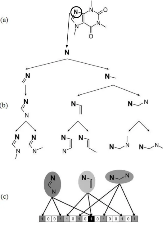
The most widespread linear notation currently in use is SMILES (Simplified Molecular Input Entry System). It is simple, easy to use and understand. Only a few rules are needed in order to write most SMILES strings (Leach & Gillet, 2007; Toropov & Benfenati, 2007; Brown, 2009; Polanski, 2009; Sammadar et al. 2015). This encoding system can be found in Appendix A. An example of SMILES notation for the caffeine molecule can be seen in Figure 6a.

Connection tables and SMILES notations can be constructed in many different ways. For example with SMILES, one can start writing the alphanumeric string starting at any atom and follow a different sequence through the molecule. Same issue can arise with a connection table as one can specifically select to number the atoms in a molecule different to another one (Leach & Gillet, 2007; Brown, 2009). Therefore it is not possible to distinguish whether two SMILES notations or two connection tables are similar. To solve this problem, the Canonical (standardised) representation was introduced so that the atoms in a molecular graph would be ordered in a unique manner. Such representations manifest themselves in code systems such as IUPAC (International Union of Pure and Applied Chemistry) and InChi (International Chemical Identifier) which can uniquely encode a molecule in very compact form (Brown 2009; Fuchs et al. 2015; Heller et al. 2015).

(41)

11

2.2. Searching for Compounds in Databases

A significant aspect to consider in Chemoinformatics is the design of Databases, which is necessarily high specific of this setting due to the complexity of the information stored. Databases that hold information about chemical structures tend to be specialised due to the nature of the methods which are used to store and manipulate the chemical structures. One can query a database containing chemical structures in order to find similar molecules. Brown (2009) defines this issue as “the rationalisation of a large number of compounds so that only the desirable remains”.

2.2.1. Structure and Sub-Structure Searching

Molecules can be sought in a database based on their structure. For this to happen, the user query needs to be translated into a standard representation (relevant to the database). If the database is arranged in a way so that Hash-Keys correspond to the locations of structures, then information retrieval can happen almost immediately by comparing the key produced from the query to the database structure-key. Sometimes however there is a slight chance that one hash-key can match to more than one structure. This phenomenon will be explained further on in the literature when describing hash-key fingerprints.

An alternative way to search for structures which also decreases the search time is looking for specific sub-structure(s) in the molecules in a database. A chemical sub-structure is a part of a molecule; sub-structure search involves checking for the presence of a certain partial structure in the whole molecule (Willet 2009). If a query is made for a sub-structure in a set of molecules, then that specific sub-structure needs to appear completely in the matching molecule (Schomburg et al. 2013). The molecules in the database being searched either match the query or not (Hood et al. 2015). This action removes the molecules that do not contain that sub-structure. Afterwards the more time-consuming sub-structure search algorithms (i.e. graph isomorphism) can be applied to the remaining molecules to see which of them truly match the query (Leach & Gillet 2007; Brown 2009). A chemical sub-structure must not be confused with a chemical pattern. A chemical pattern can be a generic or highly specific description of a chemical function. Chemical functions are used in

(42)

12 many contexts, mainly to comprehensively describe a large collection of sub-structures (Schomburg et al. 2013).

Structure and sub-structure searching involve the design of a precise query and are useful for selecting compounds that have not yet been screened from a database but they have some limitations:

• The formulation of the query can be complex for the non-expert; one is required to have enough knowledge about a structure or sub-structure in order to be able to form a meaningful query (Lemfack et al. 2014). This can become a challenge when only a few active compounds are known.

• When performing this kind of search, as mentioned before, the molecules either match the query or they do not. As a result the database is effectively partitioned into two sections (matched items and non-matched items), but there exists no relative ranking of the compounds in comparison to the structure in question (Leach & Gillet 2007). In other words the output is not ranked in any way other than by the date the database was accessed (Willet 2009).

• User has no control over the volume of the output. This means that if the query is too general there can be a large number of hits, and if the query is too specific, the output could be very small and limited (Willet et al. 1998).

In order to overcome these drawbacks, an alternative method was developed called “Similarity Searching” (Downs & Willet 1996) which allows for a more flexible molecular database search; as discussed in the next sub-section. Similarity searching suffers from none of the drawbacks mentioned for sub-structure searching.

2.2.2. Similarity Searching

The concept of similarity plays an important role in Chemoinformatics (Maggiora & Shanmugasundaram 2011; Willet 2014). Similarity (fuzzy) searching is an alternative and complimentary to exact (structure and sub-structure) searching; it retrieves the exact matches to the query object and other similar ones (Monev 2004). Here a query is used to search a database for compounds that are most similar to it (Leach & Gillet 2007). A ranked list is then generated according to the similarity to the query compound. This allows the results to be ordered based on the likelihood that they would produce the same effects as the reference compound (Brown 2009).

(43)

13 Similarity searching is used within the family of techniques called virtual screening which we shall discuss in the next section.

Similarity searching is based on the Similarity Property Principle first enunciated by Johnson and Maggiora (1990), which assumes that molecules which are structurally similar to the query molecule have similar properties i.e. biological activity (Monev 2004; Brown 2009). Also according to the principle, a similar molecule which is higher in the ranking is more likely to be active than another molecule at a lower level (Willett 2006). However in some cases structurally similar molecules have shown similar biological activities and some dissimilar molecules have shown similar biological activity (Medina-Franco 2012; Rivera-Borroto 2016). But this does not invalidate its use in drug discovery. After all if it were not for some relationship between chemical similarity and biological activity of two molecules, it would be really difficult to formulate approaches for drug discovery which take into account the structures of molecules (Willet 2009).

Assessing the extent of similarity is a pure subjective matter (Leach & Gillet 2007); there are thus no “hard and fast” rules. The methods used to measure the similarity between two molecules require three components (Willet 2009; Bajorath 2011; Willet 2014):

1) The molecular representation or descriptor: For characterising the two molecules being compared.

2) The weighting scheme: Used to assign the relative importance of the different parts of the representation.

3) The similarity coefficient: This component is used to measure the similarity between two molecules based on their appropriately weighted representations.

These components control the effectiveness of the search. A more detailed explanation for the components mentioned is provided next.

2.2.3. Molecular Representation

Molecules contain many features (properties). On their own, the individual features are not particularly informative. However a combination of them will provide a better and richer characterisation of the molecule being studied. Molecular descriptors are descriptions of molecules that aim to characterise the most noticeable aspects of a molecule (Leach & Gillet 2007; Brown 2009). They are the final results

(44)

14 of logic and mathematical procedures which transform the chemical information encoded in the structure of a molecule, into useful numbers (Todeschini & Consonni 2009; Yap 2011).

Representation (describing) of molecules means converting molecules into a series of bits that can be easily read and interpreted by computers. Todeschini & Consonni (2009) define it as a way that a molecule is symbolically represented using specific formal procedures conventional rules. Under the concept of similarity, this involves a series of comparisons between a structure or sub-structure query (the reference molecule) and an unknown molecule from a database. Molecular descriptors are of high importance in Chemoinformatics since generating them allows chemical structure information to be statistically analysed (Brown 2009; Yap 2011). There are different techniques for representing chemical molecules. Many authors (Leach & Gillet 2007; Todeschini & Consonni 2009; Bajorath 2011; Warr 2011; Willet 2014) have classified these techniques into three main groups:

1) Whole molecule descriptors (1D)

2) Descriptors that can be calculated from 2D representations of the molecule 3) Descriptors that are calculated from 3D representations of the molecule

2.2.4. 1D Molecular Descriptors

Whole molecule descriptors are measured or computed numbers which describe bulk molecular properties such as the molecular weight or the number of rotatable bonds. 1D descriptors (on their own) do not allow for meaningful comparison between different molecules. Therefore a molecule is normally represented by many such descriptors (Bajorath 2011; Willet 2014).

2.2.5. 2D Molecular Descriptors

2D molecular descriptors are calculated from a chemical structure diagram called the connection table (explained earlier on) which details all of the atoms and bonds in a molecule. The most important 2D molecular descriptors are topological indices and fragment sub-structures. A topological index is a single number that characterises a structure according to its size and shape (Bajorath 2011). Sub-structure based descriptors characterise a molecule by the sub-structural features it has, either with the help of the molecules 2D chemical graph or by its fingerprints.

(45)

15 Currently different 2D molecular descriptors exist, each from distinct descriptor classes. Brown (2009) categorises molecular descriptors into two main classes, Information-based and Knowledge-based descriptors. Information-based descriptors describe what we have. These types of descriptors tend to capture as much as possible information within a molecular representation. On the other hand knowledge-based descriptors describe what we expect. The descriptors that calculate molecular properties based on existing data or models based on such data are of the knowledge-based type.

When searching for chemical molecules of interest (to the user) in a large chemical database, the use of sub-structure searching is often time-consuming and slow because it is a nondeterministic polynomial time problem. For this reason, most chemical databases use a widely used two-stage approach sub-structure search in order to save time and quickly filter out non-matching ones. The aim is to discard and eliminate most of the molecules that cannot possibly match the sought structure. The molecules which remain are then subjected to the more sluggish sub-structure searching algorithms (Leach & Gillet 2007; Brown 2009). This elimination process is assisted by the use of molecule screens. Molecule screens are binary string representation of the molecules and the query sub-structure and they are called bit-strings (Leach & Gillet 2007). Bit-bit-strings are sequences of zero(s) and one(s); a one shows the presence of a structural feature and a zero shows its absence. The great advantage about using bit-strings is that they are the natural currency of computers and therefore can be very quickly manipulated and compared. If a feature is present in the query sub-structure (bit is set to 1) and the corresponding bit in the molecule is set to zero (feature is absent) then from the bit-string comparison it is clear that the molecule does not contain the sub-structure in question and cannot be selected. The opposite does not hold as there can be features in the molecule that are not present in the query sub-structure. These bit-strings are vector-based representations which can also be referred to as fingerprints.

Most binary screening methods are performed using one of the following two approaches:

1. Using a Structural-Key fingerprint 2. Using a Hash-Key fingerprint