Evaluation of Machine Learning
Algorithms for Lake Ice Classification
from Optical Remote Sensing Data
by
Yuhao Wu
A thesis
presented to the University of Waterloo in fulfillment of the
thesis requirement for the degree of Master of Science
in Geography
Waterloo, Ontario, Canada, 2020
AUTHOR'S DECLARATION
I hereby declare that I am the sole author of this thesis. This is a true copy of the thesis, including any required final revisions, as accepted by my examiners.
Abstract
The topic of lake ice cover mapping from satellite remote sensing data has gained interest in recent years since it allows the extent of lake ice and the dynamics of ice phenology over large areas to be monitored. Mapping lake ice extent can record the loss of the perennial ice cover for lakes located in the High Arctic. Moreover, ice phenology dates, retrieved from lake ice maps, are useful for assessing long-term trends and variability in climate, particularly due to their sensitivity to changes in near-surface air temperature. However, existing knowledge-driven (threshold-based) retrieval algorithms for lake ice-water classification that use top-of-the-atmosphere (TOA) reflectance products do not perform well under the condition of large solar zenith angles, resulting in low TOA reflectance. Machine learning (ML) techniques have received considerable attention in the remote sensing field for the past several decades, but they have not yet been applied in lake ice classification from optical remote sensing imagery. Therefore, this research has evaluated the capability of ML classifiers to enhance lake ice mapping using multispectral optical remote sensing data (MODIS L1B (TOA) product).
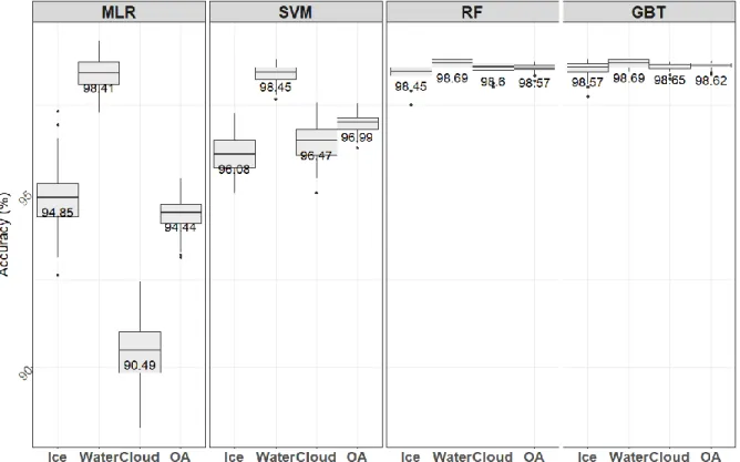
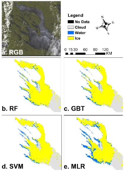
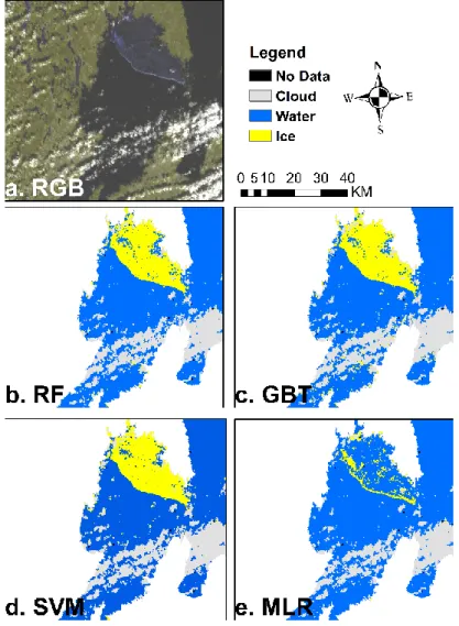
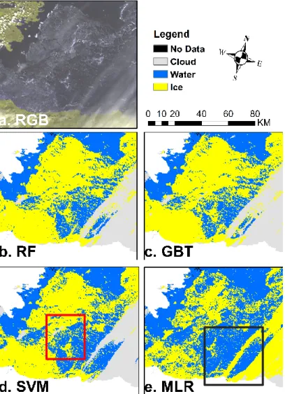
Chapter 3, the main manuscript of this thesis, presents an investigation of four ML classifiers (i.e. multinomial logistic regression, MLR; support vector machine, SVM; random forest, RF; gradient boosting trees, GBT) in lake ice classification. Results are reported using 17 lakes located in the Northern Hemisphere, which represent different characteristics regarding area, altitude, freezing frequency, and ice cover duration. According to the overall accuracy assessment using a random k-fold cross-validation (k = 100), all ML classifiers were able to produce classification accuracies above 94%, and RF and GBT provided above 98% classification accuracies. Moreover, the RF and GBT algorithms provided a more visually accurate depiction of lake ice cover under challenging conditions (i.e., high solar zenith angles, black ice, and thin cloud cover). The two tree-based classifiers were found to provide the most robust spatial transferability over the 17 lakes and performed consistently well across three ice seasons, better than the other classifiers. Moreover, RF was insensitive to the choice of the hyperparameters compared to the other three classifiers. The results demonstrate that RF and GBT provide a great potential to map accurately lake ice cover globally over a long time-series.
Additionally, a case study applying a convolution neural network (CNN) model for ice classification in Great Slave Lake, Canada is presented in Appendix A. Eighteen images acquired during the the ice season of 2009-2010 were used in this study. The proposed CNN produced a 98.03% accuracy with the testing dataset; however, the accuracy dropped to 90.13% using an independent (out-of-sample) validation dataset. Results show the powerful learning performance of the proposed CNN with the testing data accuracy obtained. At the same time, the accuracy reduction of the validation dataset indicates the overfitting behavior of the proposed model. A follow-up investigation would be needed to improve its performance. This thesis investigated the capability of ML algorithms (both pixel-based and spatial-based) in lake ice classification from the MODIS L1B product. Overall, ML techniques showed promising performances for lake ice cover mapping from the optical remote sensing data. The tree-based classifiers (pixel-based) exhibited the potential to produce accurate lake ice classification at a large-scale over long time-series. In addition, more work would be of benefit for improving the application of CNN in lake ice cover mapping from optical remote sensing imagery.
Acknowledgments
I wish to express my deepest appreciation to my thesis supervisor Dr. Claude Duguay for his patient and expert guidance over the past three years (from undergraduate to Master’s). I am extremely grateful for all his contributions of time, immense ideas, and continued encouragement to support my M.Sc. research as well as the numerous opportunities that he gave me ranging from conferences, workshops, and involvement in a number of projects. I would also like to thank Dr. Linlin Xu for his valuable insights, suggestions and discussions. I would like to acknowledge Dr. Grant Gunn for his participation on my thesis committee.
I am also indebted to all group colleagues at “Team Duguay” for stimulating discussions. Meanwhile, I mourn the loss of our colleague and friend, Marzieh Foroutan. Additionally, a special thanks to all my friends I have met during my time at the University of Waterloo. In particular, the CNU squad, including Junqian Wang, Liuyi Guo, and Yue Zhao, has actively supported me as a family since my first day at Waterloo. My gratitude goes to all those friends outside of academics during this journey as well. A special gratitude also goes to Mitch Wang for his guide, support, and encouragement. I must thank Jane Russwurm, a writing specialist, who has expertly and patiently taught me a variety of writing knowledge and skills. Last but not the least, I would like to pay gratitude to my parents for their selfless love, endless encouragement, and sincere faith. Without them, none of this could happen.
Table of Contents
AUTHOR'S DECLARATION ---ii
Abstract --- iii
Acknowledgments --- v
List of Figures --- viii
List of Tables--- x
List of Abbreviations --- xi
Chapter 1 General Introduction --- 1
1.1 Motivation --- 1
1.2 Significance of proposed research --- 2
1.3 Research objectives --- 3
1.4 Thesis structure --- 4
Chapter 2 Background --- 5
2.1 Lake Ice --- 5
2.1.1 Lake Ice Phenology --- 5
2.1.2 Recent Trends in Lake Ice Phenology --- 8
2.1.3 The Need for Monitoring Lake Ice by Remote Sensing --- 9
2.2 Optical Remote Sensing of Lake Ice --- 10
2.2.1 Optical Properties of Lake Ice --- 10
2.2.2 Reviews of Lake Ice Cover Retrieval Approaches --- 13
2.2.3 Challenges for Lake Ice Classification --- 16
2.3 MODIS Level 1B Product --- 17
2.4 Machine Learning in Remote Sensing --- 18
2.4.1 Review of Machine Learning for Ice Classification --- 18
2.4.2 Applications of Machine Learning --- 22
Chapter 3 Mapping Lake Ice Cover from MODIS Using Machine Learning Approaches --- 25
3.1 Introduction --- 25
3.2 Data and methods --- 27
3.2.2 Variable selection and variable importance measurement--- 29
3.2.3 Machine learning algorithms --- 31
3.2.4 Cross-validation strategies --- 34
3.3 Results and discussion --- 36
3.3.1 Comparison of variables combinations --- 36
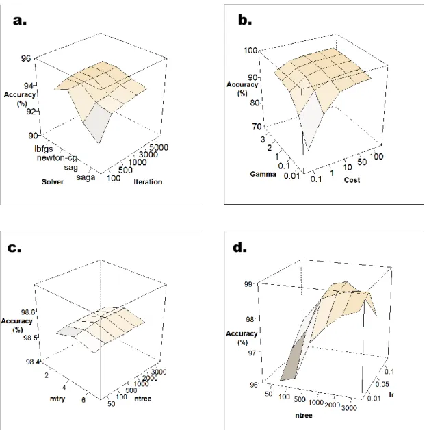
3.3.2 Sensitivity to classifier hyperparameters --- 39
3.3.3 Statistical and visual accuracy assessments --- 42
3.3.4 Spatial and temporal transferability assessments --- 50
3.4 Conclusion --- 52
Chapter 4 General Conclusion --- 54
4.1 Summary --- 54
4.2 Limitations and Recommendations for Future Work --- 55
Appendix A. Lake Ice Classification from MODIS TOA Reflectance Imagery Using A Convolutional Neural Network: A Case Study of Great Slave Lake, Canada --- 57
I. Introduction --- 57
II. Study area and data --- 58
III. Methodology --- 59
i. Preprocessing --- 59
ii. Input band configurations --- 59
iii. CNN Architecture --- 60
IV. Results and discussion --- 62
i. Band Configuration Comparison --- 62
ii. Testing and Validation Accuracy Comparison --- 62
V. Conclusions and Future Work --- 64
List of Figures
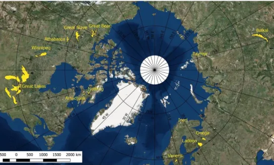
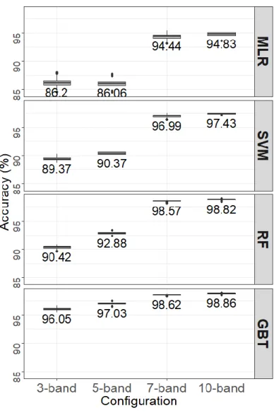
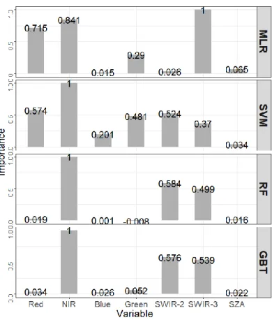
Figure 2-1 Spectral reflectance factor of lake ice in VIS and NIR range. Figure reproduced based on observations by Bolsenga (1983). ... 11 Figure 2-2 Types of ice present on shallow sub-Arctic lakes, Churchill, Manitoba: (a.) snow (white) ice; (b.) clear (bubble-free) ice. Source: Duguay et al. (2002). ... 13 Figure 3-1 Lakes in the study shown in WGS 84/Arctic Polar Stereographic projection ... 28 Figure 3-2 Comparison of classification accuracies (%) obtained with different band configurations across classifiers. ... 38 Figure 3-3 Comparison of permutation-based variable importance for the input bands across classifiers based on 7-band configuration. ... 39 Figure 3-4 Comparison of classification accuracies (%) as a function of classifier hyperparameters based on 7-band configuration. (a) MLR, (b) SVM, (c) RF, and (d) GBT. 40 Figure 3-5 Comparison of accuracies (%) obtained using random 100-fold CV across classifiers for the ice, water and cloud classes individually, and overall (OA). ... 43 Figure 3-6 Ice maps of Lake Onega (Russia) during break-up (11 May 2003, UTC 09:25) produced by the four classifiers. (a) RGB false color composite, (b) RF, (c) GBT, (d) SVM, and (e) MLR. ... 46 Figure 3-7 Ice maps of Lake Vänern (Sweden) during break-up (30 March 2003, UTC 10:30) produced by the four classifiers. (a) RGB false color composite, (b) RF, (c) GBT, (d) SVM, and (e) MLR. ... 47 Figure 3-8 Ice maps of Great Slave Lake (Canada) during break-up (5 June 2003, UTC 19:15) produced by the four classifiers. (a) RGB false color composite, (b) RF, (c) GBT, (d) SVM, and (e) MLR. ... 48 Figure 3-9 Ice maps of Great Slave Lake (Canada) during freeze-up (2 December 2009, UTC 18:50) produced by the four classifiers. (a) RGB false color composite, (b) RF, (c) GBT, (d) SVM, and (e) MLR. The black pixels correspond to no data (NaN value in input spectral bands). ... 49 Figure A-1 The location of Great Slave Lake, Canada. ………..58
Figure A-2 Lake ice cover maps produced by the processed CNN. Left: Example during break-up period (15 May 2010, UTC 2000; top: RGB composite image from MOD02 product bands 1 and 2; bottom: Lake ice map from CNN); Right: Example during freeze-up period (15 November 2009, UTC 1945; top: RGB composite image from MOD02 product bands 1 and 2; bottom: Lake ice map from CNN). ... 63
List of Tables
Table 2-1 Studies on ice classification by ML approaches ... 21
Table 3-1 List of lakes selected for this study. ... 29
Table 3-2 MODIS band configurations. ... 30
Table 3-3 Classifier functions of the scikit-learn package and their hyperparameters ... 34
Table 3-4 The clusters for spatial CV ... 36
Table 3-5 Accuracy assessment using spatial CV for lake clusters across classifiers. MA: mean accuracy, SD: standard deviation. The maximum accuracy in each cluster is bold. ... 51
Table 3-6 Accuracy assessment using temporal CV in the clusters across classifiers. MA: mean accuracy, SD: standard deviation. The maximum accuracy in each ice year is bold. ... 51
Table A-1 MODIS band configuration. …….………...59
Table A-2 Architecture of the proposed CNN. ... 61
List of Abbreviations
AMSR Advanced Microwave Scanning Radiometer AO Arctic OscillationAOI Areas of interest
BPNN Back-propagation neural network CLIMo Canadian Lake Ice Model
CNN Convolutional neural network Conv Convolutional layer
CV Cross-validation DA Discriminant Analysis DT Decision tree
ECV Essential climate variable ENSO El Ninõ/Southern Oscillation GBT Gradient boosting trees
GEOS Geostationary Operational Environmental Satellite GLCM Gray Level Co-occurrence Matrix
HDF Hierarchical Data Format
IRGS Iterative region growing using semantics KNN K-Nearest Neighbors
lr Learning rate
MA Mean accuracy
MAE Mean absolute error ML Machine Learning
MLR Multinomial logistic regression
MODIS Moderate Resolution Imaging Spectroradiometer mtry The number of variables available to a split NAO North Atlantic Oscillation
NIR Near infrared NP North Pacific ntree The number of trees OA Overall accuracy
PBVI Permutation-based variable importance PCA Principal Component Analysis
PDO Pacific Decadal Oscillation PNA Pacific North American Pool Max-pooling layer ReLU Rectified linear unit RF Random forest
RMSE Root mean square error SD Standard deviation
SSM/I Special Sensor Microwave/Imager SVM Support vector machine
SWIR Shortwave infrared SZA Solar zenith angle TIR Thermal infrared TOA Top-of-the-atmosphere TP Tibetan Plateau
VIIRS Visible Infrared Imaging Radiometer Suite
Chapter 1
General Introduction
1.1 Motivation
Lakes occupy approximately 2% of the Earth’s landscape (Brown and Duguay, 2010), and a
total of about 3.3% of the land surface above latitude 58°N is seasonally ice covered (Duguay et al., 2015). Hence, lake ice is a major component of the cryosphere due to its large areal coverage in the high latitude regions. The extent and duration of lake ice cover have wide-ranging socio-economic impacts such as navigation, winter transportation, resource development, and distribution of drinking water (Benson et al., 2012; Brown and Duguay, 2010). In addition, lakes provide habitat for several floral and faunal species. The presence of lake ice has a significant effect on the composition and abundance of aquatic species (Livingstone, 1997). Lake ice also affects water-column oxygen concentration and water temperature by limiting heat and gas exchanges with the atmosphere. A reduction in the length of ice cover seasons may facilitate greater emissions of microbial methane (Greene et al., 2014), which could further accelerate climate warming due to its role as a potent greenhouse gas. The spread of human-made pollutants (e.g. perfluorinated chemicals) is also influenced by the presence and absence of lake ice (Veillette et al., 2012; Wrona et al., 2016).
Several European studies have revealed strong relationships between lake ice phenology and large-scale teleconnections, especially with atmospheric oscillation patterns such as the North Atlantic Oscillation (NAO) (Blenckner et al., 2004; George, 2007; Karetnikov and Naumenko, 2008; Korhonen, 2006). In Canada, Bonsal et al. (2006) show strongest links between the Pacific-related indices (El Ninõ/Southern Oscillation (ENSO), the Pacific Decadal Oscillation (PDO), the Pacific North American (PNA) pattern, and the North Pacific (NP) index) and ice dates over western Canada, particularly break-up dates. The impact of the NAO and the Arctic Oscillation (AO) is found to be generally less coherent over regions of Canada (Bonsal et al., 2006). Thus, variability and trends in lake ice during freeze-up and break-up can be useful indicators of climate change and variability. Additionally, the interactions of energy between atmosphere-water-ice occur during lake ice formation, growth, and decay. The processes of energy transition can significantly affect the magnitude and timing of evaporation
and precipitation rates in lake-rich and surrounding regions. Therefore, accurate estimation of lake ice cover is important for improving numerical weather forecasting in regions occupied by lakes (Brown and Duguay, 2010). Overall then, lake ice observations are useful for many biological, ecological and socio-economic purposes.
In practice, some larger lakes do not form a complete ice cover (e.g. the Laurentian Great Lakes). On the other hand, some lakes located in the Arctic do not completely melt their ice cover in some years (i.e. perennially ice-covered lakes) (Latifovic and Pouliot, 2007). A more recent study, however, suggests that these lakes may be transitioning from perennially ice-covered to seasonally ice-ice-covered such as Lake Hazen on Ellesmere Island, Canada (Surdu et al., 2016). Hence, mapping ice cover extent/area is important for climate monitoring at high latitudes, and this can be best achieved using satellite remote sensing data.
1.2 Significance of proposed research
With the surface-based lake ice network having decreased dramatically over the last three decades (Duguay et al., 2006), the use of remote sensing has become the most logical means to establish a large-scale observational network of lake ice. Optical remote sensing products provide, at present, extensive multispectral data available for lake ice cover mapping. Moderate Resolution Imaging Spectroradiometer (MODIS) products from NASA’s Terra (2000-present) and Aqua (2002-present) satellite platforms have gained popularity for mapping lake ice cover and determining ice phenology dates (freeze-up, break-up, and ice duration) because they can provide a near twenty-year record of Earth observations at a daily temporal resolution.
Various knowledge-driven (threshold-based) methods have been developed and applied on MODIS products to retrieve lake ice and examine changes in lake ice phenology. For example, studies by Gou et al. (2017), Qi et al. (2019), and Šmejkalová et al. (2016), applied threshold-based approaches to detect lake ice and monitor ice phenology events using MODIS radiance or reflectance imagery. Besides the radiance and reflectance products, numerous studies employed MODIS snow products, produced using the normalized difference snow index (NDSI), to determine lake ice phenology (Brown and Duguay, 2012; Cai et al., 2019; Kropáček et al., 2013; Murfitt and Brown, 2017). However, the knowledge-driven algorithms may not
provide adequate classification results under complex conditions. Specifically, lakes located in high-latitude regions display lower top-of-the-atmosphere (TOA) reflectance in the visible-infrared spectral range during the ice freeze-up period, due to low solar illumination (large solar zenith angle). Thus, existing threshold-based retrieval algorithms for lake ice-water classification using optical remote sensing data do not perform well under such conditions.
Machine learning (ML) approaches have been applied in many studies of ice retrieval from remote sensing imagery (Han et al., 2016; Leigh et al., 2014; Su et al., 2015). The majority of these studies have employed microwave satellite data for sea ice classification. Hence, it is imperative to understand the performance of ML to lake ice classification from optical and microwave remote sensing imagery. Three aspects need to be carefully considered when applying ML for remote sensing classification. First, variable selection and importance measurement allow further understanding of the underlying classification processes by classifiers and improve their performance. Second, hyperparameter selection must be conducted to exploit the full capability of a classifier instead of evaluating simplex classification derived with only one set of hyperparameters. Finally, since remote sensing measurements over lake ice can vary in time (e.g. daily and seasonally between freeze-up and break-up) and in space (e.g. from one lake or lake region to another), the temporal and spatial transferability of classifiers should also be examined.
1.3 Research objectives
The overall objective of this research is to evaluate the performance of machine learning (ML) classifiers for lake ice classification from optical remote sensing data. This thesis assesses different ML approaches for lake ice cover mapping using MODIS data, thereby proposing an optimal classifier for lake ice cover mapping. Specifically, three sub-objectives are to: 1) determine the optimal combination of input variables, including variable importance, to obtain robust classification results; 2) perform hyperparameter selection and examine the sensitivity of the change in the hyperparameters; and 3) investigate the suitability of ML classifiers for lake ice cover mapping across different regions of the globe and over a relatively long time period (ca. 20 years).
1.4 Thesis structure
This thesis has been written following the manuscript format where a paper is included as an individual chapter. Chapter 1 provides the motivation of this research and addresses the research objectives. Chapter 2 covers background knowledge regarding lake ice, ice classification of remote sensing, and remote sensing classification using ML. Chapter 3 contains the paper and is entitled “Mapping Lake Ice Cover from MODIS Using Machine Learning Approaches”. A short paper titled “Lake Ice Classification from MODIS TOA Reflectance Imagery Using A Convolutional Neural Network: A Case Study of Great Slave Lake, Canada” is included in Appendix A. It has been submitted for publication in Proceedings of the 2020 IEEE International Geoscience and Remote Sensing Symposium and is to be presented at the related meeting in July 2020. Finally, Chapter 4 provides conclusions and recommendations for future work.
Chapter 2
Background
This chapter is divided into three main sections designed to present the background knowledge relevant to this research. First, the mechanisms of lake ice formation and decay are addressed, followed by a review of recent trends in lake ice phenology. Then, the need for lake ice mapping by remote sensing is also argued in the first section. Section 2.2 presents an extensive introduction to optical remote sensing of ice aimed at discussing previous remote sensing methods for lake ice retrieval and highlighting current classification challenges. A description of the MODIS L1B top-of-the-atmosphere (TOA) reflectance product, the main input data used in this research, is covered in section 2.3. Finally, a review on the application of machine learning (ML) in remote sensing classification is provided to show the potential of ML algorithms for lake ice classification; algorithms that are then tested in the research manuscript included in section 2.4.
2.1 Lake Ice
2.1.1 Lake Ice Phenology
Lake ice phenology is the term used to define the stages of ice formation and decay, and the duration of ice cover on lakes. Freeze-up covers the period between initiation of ice formation on a lake surface until the time of complete ice cover, occurring in the fall and winter months (Brown and Duguay, 2010). Break-up, which is basically the progress of ice disintegration, refers to the period from the beginning of ice melt until the entire lake becomes completely ice-free, occurring in spring to summer depending on geographical location (Brown and Duguay, 2010). Ice season is defined as ice cover duration from the first day of ice presence to the day of complete ice disappearance (Kang et al., 2012).
The formation, growth, and decay of ice are affected significantly by the surplus and deficit of the energy balance at the lake surface (Williams, 1965). The energy available for ice formation and decay is influenced by three factors: heat exchange between lake and atmosphere, the heat stored in the lake, and heat import from inflows of water (Williams,
1965). The exchanges with the atmosphere are governed by climatic factors (e.g., air temperature, precipitation, wind, and radiation), whereas the amount of heat storage is mainly controlled by non-climate factors such as lake morphometry (area and depth) (Brown and Duguay, 2010).
Air temperature, in summer and fall, is the dominant climatic control on the timing of lake ice freeze-up (Williams, 1965). With more heat absorbed by the lake during ice-free months, ice formation can be delayed and vice versa. A study by Bonsal et al. (2006) indicates that freeze-up dates were delayed by up to 5 days in Western Canada during the warm anomalous years of El Niño events in the 1950 to 1999 period. When air temperatures drop in the fall, heat is lost at the surface, which causes vertical convection between the cooler denser water of the surface layer and the warmer water of the underlying layer (Brown and Duguay, 2010). With freshwater reaching its maximum density at 4℃, the lake surface cooling hampers convective overturning resulting in ice formation (Jeffries et al., 2005). Once surface water temperature has reached the freezing point, black ice, which is known as congelation ice, forms downward from the surface, generating layers of vertically orientated c-axis (column-like) ice crystals (Jeffries et al., 2005). When the weight of snow (the snow mass) is large enough to depress the ice below its hydrostatic level, water will seep through cracks in the congelation ice and wet the base of the snowpack which will result in slush formation. Slush freezing, afterward, will form snow ice, often referred to as white ice. Snow accumulation on the ice surface can also slow down the ice growth rate because it insulates the lake, thereby also reducing heat loss (Sturm et al., 1997). Additionally, during the freeze-up period, wind not only can promote the mixing of cooler water and warmer water which may delay the initial formation of skim ice (Soja et al., 2014; Williams, 1965), but it can also break the skim ice, which first forms, to delay the formation of a solid ice cover (Brown and Duguay, 2010). Another climatic variable that has been linked to ice formation and growth is cloud cover. The presence of cloud cover can lead to lower air temperatures, thus accelerating ice formation and growth, by reflecting incoming shortwave radiation away from the ice cover (Brown and Duguay, 2010; Wang et al., 2016). Conversely, Brown and Duguay (2010) indicate that clouds can trap longwave radiation to slow down ice growth by causing a warmer atmosphere, especially at night.
The process of lake ice break-up is significantly dominated by temperature via heat gain from the atmosphere and solar radiation (Brown and Duguay, 2010; Williams, 1965). The break-up period can last a few days to several weeks after the 0℃ isotherm date is reached (Duguay et al., 2006). Moreover, ice break-up shows a stronger temporal coherence with changes in air temperature, compared to ice freeze-up timing which is also strongly influence by lake morphometry (described below). Jeffries and Morris (2007) show that a ± 1℃ change in air temperature results in a ± 1.86 days change in break-up dates for Alaskan ponds. Duguay et al. (2006) indicate significantly earlier break-up occurring over Canadian lakes due to climate warming in recent decades, but did not observe an apparent pattern of changes in freeze-up dates. Furthermore, ice/on-ice snow melt can be affected by the radiative processes. The albedo of the exposed surface (ice, snow, ponding water) controls the amount of solar radiation absorbed and heat available for melting (Brown and Duguay, 2010). Albedo falls typically in the range of 0.70 to 0.90 as fresh snow accumulates on the ice, and drops to 0.28-0.54 as the presence of water increases (Heron and Woo, 1994; Howell et al., 2009; Petrov et al., 2005). Snow cover increases the albedo of the lake surface to hinder the lake from absorbing heat, resulting in a delay in the timing of break-up (Michel et al., 1986). Once the temperature rises, the melt of snow and ice occurs on the lake surface, exposing the underlying darker ice (for congelation ice) (Heron and Woo, 1994). The change of crystal orientation in the surface layer reduces the albedo so that more solar radiation is absorbed by the lake surface, meaning that more heat is available for melting (Brown and Duguay, 2010; Heron and Woo, 1994). In addition to the radiative actions, wind also affects the break-up event since the mechanical process will lead to ice disintegration and the formation of large cracks (Williams, 1965).
The timing of lake ice phenology is additionally impacted by non-climatic factors including lake morphometry, lake elevation, and water inflow to the lake. Lake morphometry, linked to factors such as lake depth, area, volume, and fetch, determines the amount of heat storage in the water body that affects the time needed for the lake to lose heat and eventually freeze (Brown and Duguay, 2010; Korhonen, 2006). Deeper lakes can accumulate more heat during ice-free seasons (i.e. summer and fall) due to their large thermal inertia (Choiński et al., 2015).
Moreover, lake fetch, which is the longest distance over the lake surface that can generate wind-driven waves, influences the event of ice formation (Jeffries et al., 2012). At the initial timing of ice formation, the average bulk temperature on small lakes is around 2 to 3℃, which is higher than the bulk temperature on large lakes (lower than 1℃) (Jeffries et al., 2005; Scott, 1964). The relationship between lake elevation and lake ice phenology has been described in a few studies (Brown and Duguay, 2010; Livingstone et al., 2010; Williams and Stefan, 2006). For example, Livingstone et al. (2010) reported ice cover duration increasing by 10.2 days per 100 m altitude on alpine lakes, whose elevations range from 1,581 to 2,157 meters above sea level, located in the Tatra Mountains, Poland. Water generated from rivers or land runoff affects the ice events of break-up and freeze-up by breaking ice cover mechanically (Brown and Duguay, 2010; Howell et al., 2009; Williams, 1965).
2.1.2 Recent Trends in Lake Ice Phenology
The timing and duration of lake ice events are the main metrics sensitive to weather and climate conditions, thus ice phenology can be considered as a powerful indicator of climate change and variability (Duguay et al., 2014, 2006; Mishra et al., 2011). Trends in lake ice phenology over the Northern Hemisphere have attracted public interest recently for studies of climate change at large spatial scales. A study by Magnuson et al. (2000), examining the changes in the freshwater ice events from 1846 to 1995, shows a trend of 5.8 days later per decade for ice freeze-up and 6.5 days earlier per decade for ice break-up around the Northern Hemisphere. Benson et al. (2012) performed a linear regression analysis of ice phenology variables using the dataset of 75 Northern Hemisphere lakes over the period of 1855-2005. Their study shows 0.3-1.6 days per decade trend towards later for freeze-up, 0.5−1.9 days per decade trend for earlier for break-up, and 0.7−4.3 days per decade trend towards shorter ice duration. A recent study by Du et al. (2017) reveals trends towards later ice-on dates in 43 of 73 study lakes located in the Northern Hemisphere among the period of 2002-2015, also demonstrating an increasingly shorter ice cover season. Meanwhile, they also indicate a latitudinal pattern of the changing trends. Specifically, lakes at higher latitudes (> 60° N) are more likely to experience trends of earlier ice break-up and shorter ice seasons compared to lakes at lower latitudes (<
50° N) (J. Du et al., 2017). A prediction study on future trends of lake ice phenology by Dibike et al. (2012) shows that freeze-up will shift later by 5-20 days and break-up will shift earlier by 10-30 days around the Northern Hemisphere by 2040-2079 when compared to the baseline period of 1960 – 1999. The above analyses, as well as others, have indicated that warming climate conditions have led to the earlier occurrence of lake ice break-up dates broadly over the Northern Hemisphere.
Several recent studies also present trends of lake ice phenology over more specific regions. Choiński et al. (2015) describe trends in later formation of complete ice cover and earlier disappearance of ice over 18 polish lakes between 1961 and 2010. Brown and Duguay (2011) performed simulations of lake ice phenology over the North America Arctic region applying the Canadian Lake Ice Model (CLIMo). The simulation results reveal a 10–30 day reduction for the ice cover duration by 2041-2070, compared to the period of 1961–1990. Cai et al. (2019a) analyze the characteristics of ice phenology over 58 lakes on the Tibetan Plateau from 2001 to 2017. This study indicates that the freeze-up events have been delayed and ice cover duration has become shorter over the majority of the study lakes (Cai et al., 2019a). Furthermore, changing patterns of ice phenology associated with later freeze and shorter ice cover duration have been found in other studies on lakes located on the Tibetan Plateau (Gou et al., 2017; Qi et al., 2019) and Northeast China (Yang et al., 2019).
2.1.3 The Need for Monitoring Lake Ice by Remote Sensing
Diverse methods have been proposed for monitoring lake ice phenology, including surface-based (government agencies or volunteers) and satellite-surface-based networks (Brown and Duguay, 2010, 2012; Duguay et al., 2014; Jeffries and Morris, 2007). Nationally, surface-based networks have mainly been supported by operations at meteorological or hydrological stations (Brown and Duguay 2010). However, the stations are distributed unevenly and sparsely with limited records available to support studies over remote regions. In addition, a cutback in surface-based observational networks has unfortunately occurred globally since the 1980s (Duguay et al., 2006; Key et al., 2007). The volunteer-based networks require volunteer observers to collect data for lake ice with digital camera imagery (Dyck, 2007; Jeffries and
Morris, 2007). Monitoring lake ice from the volunteer-based networks is challenging for two reasons. First, since lake ice can freeze and melt multiple times in winter and spring, definitive freeze-up and break-up dates are difficult to determine (Futter, 2003). Another reason is that long-term and wide-scale monitoring requires a lot of volunteers who will hold various definitions for freeze-up and break-up (Futter, 2003). Surface-based networks operated by volunteers provide quite limited measurements depending on the human experience and the observer scope.
In contrast, remote sensing data provide large-scale and objective observations ranging from individual lakes to regional or even global scale. Hence, mapping lake ice from remote sensing data is vital to assess lake ice phenology over large spatial scales and over increasingly longer time periods.
2.2 Optical Remote Sensing of Lake Ice
2.2.1 Optical Properties of Lake Ice
Lake ice is a relatively translucent material with an intricate structure and complex optical properties. The term “optical” refers to the portion of the electromagnetic spectrum of the wavelength (shortwave) range of radiation from the sun (roughly 0.25 to 2.50 µm). Understanding the reflection, absorption, and transmission of shortwave radiation by lake ice is useful to drive lake ice classification from optical remote sensing imagery. The optical properties of lake ice vary with ice type, the bubble content of ice, and incident radiation.
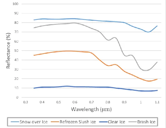
Due to various physical structures, lake ice exhibits a variety of optical characteristics. A pilot study by Bolsenga (1969) investigated the broadband albedo (0.3~3.0 µm) of various types of snow-free ice over the Great Lakes at solar elevations ranging from 32° to 40°. Albedo ranged from 0.10 for clear ice to 0.46 for snow ice. Refrozen slush ice and brash ice also showed high albedos above 0.40, which are slightly higher than that of pancake ice (0.31) and slush curd ice (0.32). In a subsequent study by Bolsenga (1983), the spectral reflectance signatures of lake ice types from 0.340 to 1.100 µm were examined. Figure 2-1 shows selected results from Bolsenga (1983) (i.e., brash ice, refrozen slush ice, and clear ice). Overall, the spectral reflectance of lake ice types is quite uniform across the visible spectrum. There is a
slight rise from 0.340 to 0.550 µm and a faint decline from 0.550 to 0.700 µm, forming a wave peak at around 0.550 µm; however, a rapid decrease of reflectance (approx. 0.20 – 0.30) occurs from 0.700 to 1.100 µm (Bolsenga, 1983). Likewise, the measured surface reflectance of clear ice was around 0.10 across the spectrum. Other ice types (i.e., snow ice and refrozen slush ice) have remarkably high reflection compared to clear ice. Maslanik and Barry (1987) analyzed mean digital counts of different ice and open water types recorded by Landsat Thematic Mapper (TM) channels 1-4. The results show that snow-free black ice with low reflectance was not distinguishable clearly from turbid water in the spectral range of the four channels. Additionally, congelation ice presents very high radiation transmittance from 0.77 to 0.89 in the 0.400 – 0.700 µm range (Bolsenga, 1981), accompanying low reflection.
Figure 2-1 Spectral reflectance factor of lake ice in VIS and NIR range. Figure reproduced based on observations by Bolsenga (1983).
As shown in Figure 2-2, snow ice (a.) has a white appearance, and clear ice (b.) is transparent visually. Snow ice consists of numerous spherical bubbles since air dissolved in the surface saturated water cannot be incorporated into the ice crystal lattice (Mullen and Warren, 1988). However, the concentration of bubbles in congelation ice is generally low for water bodies (i.e. excluding shallow Arctic/sub-Arctic lakes). In the case of the shortwave spectrum, the scattering of light by bubbles increases the albedo over the spectral range since specular reflection exits alone (Mullen and Warren, 1988). In addition to the effect of bubbles, as mentioned previously, the crystal orientation can also affect the albedo of ice. Heron and Woo (1994) found a significant decrease of albedo from 0.45 to 0.20 during the break-up period. The removal of the c-axis vertical ice resulted in exposure of the underlying c-axis horizontal crystals. Laboratory sea ice observations reveal that the reflectance of ice increases as ice thickness increases (Perovich, 1979; Perovich et al., 1998).
Besides the effect of ice type, snow cover can also result in spectral variations of remote sensing imagery. Snow accumulation on lake ice occurs during the ice season. Snow-covered ice overall demonstrates very high reflectivity compared to snow-free ice, and thereby snow cover on top of the ice is clearly distinguishable from snow-free ice (Maslanik and Barry, 1987). According to the study by Bolsenga (1983), as shown in Figure 2-1, the reflectance values for ice are significantly lower than those of snow over ice. The variation of snow reflectance is highly dependent on grain size; specifically, snow reflectance decreases with an increase in grain size.
Optical remote sensing instruments mounted on satellites typically measure solar radiation reflected by the Earth with narrow fields of view. Hence, parameters affecting incident radiation also influence the reflectance of ice. The daily variability of ice albedo is high due to changing solar elevation (Bolsenga, 1977; Leppäranta et al., 2010). With solar zenith angle increasing, the diffuse radiation flux increases, resulting in the attenuation of the radiation flux of incident sunlight at the surface (Coakley, 2003). Therefore, top-of-the-atmosphere (TOA) reflectance is very low due to the lack of solar radiation reflected by the surface.
a. b.
Figure 2-2 Types of ice present on shallow sub-Arctic lakes, Churchill, Manitoba: (a.) snow (white) ice; (b.) clear (bubble-free) ice. Source: Duguay et al. (2002).
2.2.2 Reviews of Lake Ice Cover Retrieval Approaches
Various knowledge-driven, threshold-based, methods have been developed to retrieve lake ice from optical remote sensing imagery. The main idea of the knowledge-driven algorithms is to develop generic rules using inference from empirical observations.
The Moderate Resolution Imaging Spectroradiometer (MODIS) snow products in collection 5 (C5) and 6 (C6) also include retrieved lake ice. The MODIS snow product was developed using MODIS Level 1B (TOA), MODIS Cloud Mask products and geolocation fields. In the C5 product, snow cover was classified by a set of decision rules with the thresholds (Riggs et al., 2006) shown in equation 1.
𝑁𝐷𝑆𝐼 = (𝐵𝑎𝑛𝑑 4 − 𝐵𝑎𝑛𝑑 6) (𝐵𝑎𝑛𝑑 4 + 𝐵𝑎𝑛𝑑 6)≥ 0.4
𝐵𝑎𝑛𝑑 2 > 0.11
where Band 2: reflectance at 0.865 μm; Band 4: reflectance at 0.555 μm; Band 6: reflectance at 1.640 μm. Lake ice is detected in the C5 product using the same criteria as for snow on land and a lake mask. The Normalized Difference Snow Index (NDSI) serves as the basis for the MODIS snow product. The ice phenology retrieved by the MODIS snow C5 product from 2000 – 2011 for Quebec, Canada is comparable to the simulation derived by the 1-D Canadian Lake Ice Model (Brown and Duguay, 2012). Furthermore, the snow C5 imagery was found to present lake ice conditions similar to that of the Interactive Multi-sensor Snow and Ice Mapping System (IMS) product, produced from multiple remote sensing sources (Brown and Duguay, 2012). Chen et al. (2018) employed the MODIS snow C5 product to calculate the daily fraction of ice cover on alpine lakes of the Tibetan Plateau (TP) to detect the change of ice phenology from 2002 to 2015. Likewise, Cai et al. (2019a) applied the snow products from Aqua and Terra to determine ice phenology over eight lakes on the TP using the same calculation method of ice fraction. The accuracy of the MODIS snow cover products has been validated against other sources (i.e., Landsat imagery, AMSR-E/2, SSM/I), and shows varying agreements (Cai et al., 2019a). Moreover, using the MODIS snow C5 products, Murfitt and Brown (2017) investigated short term trends in lake ice phenology for Ontario and Manitoba in Canada. The validation results against in-situ data show an average mean absolute error (MAE) of 9 days for both ice-on and ice-off dates (Murfitt and Brown, 2017). In addition to the daily snow product, the MODIS 8-day composite snow products in C5 have been used to monitor lake ice phenology over the TP region (Kropáček et al., 2013).
Compared to the snow C5 product, the MODIS snow C6 product presents a NDSI value higher than 0 in each pixel (Riggs and Hall, 2015). Moreover, a number of data screens have been developed as filter criteria to further identify snow (Riggs and Hall, 2015). When any pixel with a valid NDSI value fails on one of the screens, the pixel is flagged as no snow or uncertain snow (Riggs and Hall, 2015). The MODIS snow C6 product has been applied to determine lake ice phenology using band thresholds on the TP (Qiu et al., 2019), Northeast China (Yang et al., 2019), and Xinjiang, China (Cai et al., 2019b). However, the classification by the MODIS snow product shows confusion between clouds and ice/snow due to the occurrence of omission when the MODIS cloud mask misclassifies regions of snow/ice as a
certain cloud. Similarly, the retrieval algorithm using NDSI was applied using the Visible Infrared Imaging Radiometer Suite (VIIRS) to perform lake ice classification with bias range from 0.25% to 3.2% in comparison with the AMSR2 product (Dorofy et al., 2016).
Besides the MODIS snow products, the MODIS surface reflectance product has been employed commonly to examine lake ice phenology. Šmejkalová et al. (2016) built daily surface-reflectance time series for 2000–2013 from MODIS band 2 (0.865 μm) data to determine ice phenology in the Arctic region. The results present a root-mean-square-error (RMSE) of 6.16 days in comparison to in-situ data; the authors also indicate that cloud cover and low sun angle during freeze-up significantly affect the quality of the estimation (Šmejkalová et al., 2016). A threshold-based approach using MODIS bands 1 (0.645 μm) and 2 (0.865 μm) was developed to discriminate lake ice and open water, thus identifying ice phenology events on the TP with combing the MODIS surface temperature products (Gou et al., 2017). Furthermore, the MODIS snow product has been utilized with surface reflectance bands 3-5 to calculate the ice fraction in the study area (Gou et al., 2017). In this research, a pixel is classified as ice only if all three sources indicate ice, resulting in cautious perdition (Gou et al., 2017). Likewise, Qi et al. (2019) developed another threshold-based algorithm using MODIS surface reflectance bands 1 and 2 for ice monitoring on Qinghai Lake. However, instead of applying two bands respectively, the difference between bands 1 and 2 was used as a criterion of the algorithm to label pixels as lake ice (Band 1 − Band 2 > 0.028); another criterion was a threshold of band 1 only (Band 1 > 0.05) (Qi et al., 2019). Additionally, Zhang and Pavelsky (2019) used dynamic thresholds of MODIS band 2 to discriminate lake ice based on the size of lakes.
The MODIS top-of-the-atmosphere (TOA) reflectance product was applied by Reed et al. (2009) to provide a more accurate lake ice classification by manual interpretation as compared to various digital analysis techniques. The TOA reflectance product has also been combined with MODIS sea surface temperature data to identify the occurrence of water-clear-of-ice by a threshold-based approach for Lake Baikal, Russia (Nonaka et al., 2007). Making use of Geostationary Operational Environmental Satellite GOES imagery, Dorofy et al. (2016) identified two lake ice classes (i.e., thick ice, gray ice) in the Great Lakes region by a
threshold-based approach developed using Mid-Infrared Sea and Lake Ice Index (MISI), incorporating reflectance of the mid-infrared and visible bands. They indicated that MISI considers the spectral differences between thick ice and the relatively darker, gray ice so that it is useful for distinguishing the two types of lake ice (Dorofy et al., 2016).
The knowledge-driven algorithms have generally exploited variations of the optical properties of ice, water, and cloud to define specific spectral criteria to classify these features. NDSI has not only been employed for the development of the MODIS snow product, but also utilized as the main means to perform lake ice estimation from optical remote sensing data. Additionally, the ability of ice to reflect high radiation of NIR wavelengths (MODIS band 2) to the atmosphere was found as a useful characteristic for detecting lake ice from open water, having therefore been used for lake ice investigations frequently (Oke, 1987; Svacina et al., 2014). However, the varying agreements of the MODIS snow products and validation data indicate the limitation of lake ice classification from the products. Moreover, most studies using the MODIS reflectance products to classify lake ice employed the MODIS cloud mask, known as MOD35, to filter cloudy pixels. However, previous assessments of the MODIS snow and cloud products have shown confusion between ice and cloud (Hall and Riggs, 2007; Leinenkugel et al., 2013; Tekeli et al., 2005). The confusion significantly affects the quality of lake ice cover estimations.
2.2.3 Challenges for Lake Ice Classification
A series of knowledge-driven algorithms have been developed to monitor lake ice in many regions. However, the existing knowledge-driven algorithms have difficulties dealing with complex conditions to provide highly accurate classification results. For example, the condition of high solar zenith angles in high-latitude regions results in lower TOA reflectance over lakes in the visible-infrared spectral range during the ice freeze-up period. Thus, threshold-based retrieval algorithms for lake ice-water classification using TOA satellite data do not perform well under such a condition. Šmejkalová et al. (2016) indicated that freeze-up dates for high latitude lakes are difficult to identify due to problems with high solar zenith angles. High solar zenith angles prevent the solid classification of snow/ice cover, which is
important when studying freeze-up at northern latitudes (Brown and Duguay, 2012). Moreover, traditional threshold-based approaches for cloud detection still face severe challenges over ice-covered areas in the Arctic and sub-Arctic (Chen et al., 2018). As pointed out earlier, the confusion between ice and cloud exists in the MODIS cloud product, therefore introducing uncertainty in lake ice maps (Hall and Riggs, 2007; Leinenkugel et al., 2013; Tekeli et al., 2005). The classification challenge due to the low reflectance contrast of black ice with turbid water has been indicated in numerous studies regarding ice monitoring (Bolsenga, 1983; Liu et al., 2016; Mullen and Warren, 1988; Perovich, 1979). Additionally, the threshold-based approaches significantly rely on particular sensors that are not directly applicable to data obtained with other sensors. This is especially true for cloud detection algorithms because these algorithms strongly depend on the thermal bands. However, unlike MODIS, the majority of optical remote sensing data with high spatial resolution, do not have sufficient thermal bands. Therefore, the threshold-based algorithms lack generalization ability to transfer to mutiple sensors (Hagolle et al., 2010; Roy et al., 2010).
2.3 MODIS Level 1B Product
The MODIS sensors, onboard the Terra and Aqua satellites, launched in 1999 and 2002 respectively, scan the majority of the entire Earth’s surface every day. The two satellites are in a Sun-synchronous orbit at a 705 km altitude, such as Terra at a 10:30 AM equatorial crossing time, descending node, and Aqua at a 1:30 PM equatorial crossing time, ascending node (Wolfe, 2006). MODIS takes measurements with a whiskbroom electro-optical instrument to provide scans in the along-track direction (Wolfe, 2006). Since launch, both MODIS instruments have been delivering near-continuous observations and yielding scientific and environmental products useful to study the Earth’s system of atmosphere, land, ocean, and cryosphere (Xiong et al., 2015). As shown in the last section, the MODIS products have gained popularity for delineating lake ice cover by the threshold-based algorithms.
The MODIS Level 1B (L1B) product, the main input data product used in the ML algorithms tested in this thesis, is comprised of calibrated Earth view data of 36 spectral bands ranging from 0.41 to 14.4 µm, stored in three HDF files corresponding to three spatial
resolutions. The MODIS 36 spectral bands are bands 1 and 2 at a nadir spatial resolution of 250 m, bands 3-7 at a nadir spatial resolution of 500 m, and all other bands at a nadir spatial resolution of 1 km. Specifically, bands 1-19 and 26 are the reflective solar bands, and bands 20-25 and 27-31 are the thermal emissive bands. The L1B calibrated data include TOA reflectance for the reflective solar bands, and radiances for both the reflective solar and thermal emissive bands.
The now twenty-year record of MODIS data from the Terra satellite (2000-present) is useful for investigating changes in lake ice phenology over a relatively long time period. The MODIS L1B product allows monitoring lake ice conditions at a high temporal resolution (daily). Moreover, the 36 bands provide sufficient spectral information of the Earth surface helpful to map lake ice extent. The powerful capability of Earth coverage and the highest spatial resolution of 250 m are allow for lake ice mapping at the global scale.
2.4 Machine Learning in Remote Sensing
2.4.1 Review of Machine Learning for Ice Classification
The overall challenge for lake ice mapping using optical imagery is to identify two features with similar optical properties, such as thin cloud against ice, black ice against water, turbid water against ice. Machine learning (ML) techniques, known as data-driven algorithms, are generally able to model complex class signatures with a variety of input variable data. Hence, ML classification has received considerable attention for the past several decades and researchers in the field of remote sensing are increasingly applying these classifiers for ice detection.
Several ML models have been developed for ice retrieval from Synthetic Aperture Radar (SAR) imagery. In order to provide sea ice observations with a high level of confidence for data assimilation of a climate change prediction system, Komarov and Buehner (2017) proposed a technique using logistic regression (LR) for automated detection of ice and open water using RADARSAT-2 ScanSAR images. Three input features computed from SAR and wind speed data are used in the proposed LR model. A rigorous probability threshold of 0.95 was adopted to determine ice pixels, producing 79.41% ice-class accuracy. A further study by
Komarov and Buehner (2018) introduced an adaptive probability thresholding approach to improve this technique. The authors applied sequential RADARSAT-2 imagery to examine the performance of the improved technique and indicated that 98.93% of collected sea ice observations were retrieved correctly (Komarov and Buehner, 2019). Shen et al. (2017) compared the performance of six ML classifiers for sea ice classification from Cryosat-2 data. Random forest (RF) achieved the best performance (about 90% classification accuracy), followed by Support Vector Machine (SVM), back propagation neural network (BPNN), and Bayesian, with K nearest-neighbor (KNN) performing the worst (Shen et al., 2017). SVM has been tested for detection of multiple sea ice types using RADARSAT-2 imagery with above 86% classification accuracy (Liu et al., 2015). The SVM model requires three input variables, i.e., HH, HV, and the gray-level co-occurrence matrix (GLCM) feature, which is also an approach to extract textural features (Liu et al., 2015). Due to the limited number of SAR bands, Han et al. (2017) generated 12 texture features from KOMPSAT-5 applied on a RF model, producing a 99.24% overall accuracy of ice detection in the Chukchi Sea. In addition to extracting spatial patterns with GLCM, an image segmentation technique, named iterative region growing using semantics (IRGS), was employed for sea ice retrieval from single and dual polarization SAR imagery (Leigh et al., 2014; Ochilov and Clausi, 2012). IRGS is able to minimize the impact of the incidence angle variations through conducting segmentation separately on smaller polygons (Ochilov and Clausi, 2012). Furthermore, Leigh et al. (2014) combined IRGS and SVM results using 28 textural features from dual polarization SAR imagery to map sea ice with an overall classification accuracy of 96.42%. Wang et al. (2018) applied the IRGS technique but with manual labeling on ice mapping in Lake Erie, producing an overall accuracy of 89.5% from RADARSAT-2 scenes.
Besides SAR data, optical satellite imagery has been used to perform ice classification using ML techniques. Han et al. (2018) proposed a framework combining active learning and transductive SVM for sea ice detection. The framework achieved retrieval results of above 90% accuracy from Landsat-8 and above 85% accuracy from EO-1 (Han et al., 2018). Similar to the SAR applications, Su et al. (2015) derived texture features (GLCM) and surface temperature from MODIS images for ice detection in the frozen Bohai Bay, China. SVM was
adopted to identify sea ice and open water pixels, producing an 87.13% overall accuracy. Tom et al. (2018) applied SVM to obtain an accuracy range from 75 to 100% on ice-water classification within four lakes located in Switzerland using the MODIS TOA reflectance product. Research by Barbieux et al. (2018) employed the decision tree (DT) technique to optimize a threshold-based algorithm of ice classification using radiometric indexes and TOA reflectance bands on five different lakes from the Landsat-8 OLI multispectral data. The range of accuracy varied from 93 to 97% among the selected study zones except for one showing an 84.4% accuracy (Barbieux et al., 2018). Moreover, MODIS, AMSR-E and SSM/I data were cobined to monitor landfast sea ice in the Antarctic using DT and RF (Kim et al., 2015). The accuracy assessment shows comparable results between RF (94.77%) and DT (93.09%) (Kim et al., 2015).
Overall (Table 2-1), the majority of studies applying ML techniques on ice detection are based on microwave remote sensing images, for instance RADARSAT-2 (Komarov and Buehner, 2017; Leigh et al., 2014; Liu et al., 2015), TerraSAR-X (Han et al., 2016), and Cryosat-2 data (Shen et al., 2017). Nevertheless, in fact, optical remote sensing imagery provides abundant spectral information on Earth’s surface for ice detection. Additionally, only a few studies (Barbieux et al., 2018; Tom et al., 2018; Wang et al., 2018) have explored the feasibility and performance of ML models in lake ice mapping. Actually, the retrieval of lake ice using ML algorithms from optical remote sensing data has received much less attention than for sea ice. Hence, an examination of the capability of ML algorithms for lake ice cover mapping is very much a new topic that merits investigation.
Table 2-1 Studies on ice classification by ML approaches.
Study Objective Data Algorithm Result
Barbieux et al. (2018) Lake ice classification
(5 lakes in Europe and North America) Landsat 8 OLI DT Five testing areas: 84.40% to 97.30 % Han et al. (2017) Sea ice classification
(Chukchi Sea)
KOMPSAT-5
HH-Pol. EW RF Overall accuracy: 99.24% Han et al. (2018) Multiple sea ice classification
(Baffin, Liaodong,Bohai Bays)
EO-1
Landsat-8 TSVM Three testing areas: 87 % - 97 % Kim et al. (2015) Landfast sea ice classification
(Antarctic) MODIS IST/AMSR-E
DT RF
Overall accuracy of DT: 93.09% Overall accuracy of RF: 94.77% Komarov and Buehner
(2017, 2018, 2019)
Sea ice classification (Labrador Sea & Baffin Island)
RADARSAT-2
Dual-Pol ScanSAR LR
Ice classification accuracy:79.41% (2017), 88.23% (2018), 98.93% (2019)
Leigh et al. (2014) Sea ice classification (Alaskan coast)
RADARSAT-2
Dual-Pol ScanSAR IRGS/SVM
Ice classification accuracy: 98.21% Water classification accuracy: 92.72% Liu et al. (2015) Multiple sea ice classification
(Beaufort Sea)
RADARSAT-2
Dual-Pol ScanSAR SVM
Overall accuracy of two testing areas: 91.74%, 91.43%
Shen et al. (2017) Multiple sea ice classification
(Arctic) Cryosat-2 6 classifiers
RF achieved the best, followed by SVM, BPNN, Bayesian, with KNN the worst
Su et al. (2015) Sea ice classification
(Bohai Bay) MODIS TOA (L1B) SVM Overall accuracy: 84.73% Tom et al. (2018) Lake ice classification
(4 Swiss lakes)
MODIS TOA (L1B)
VIIRS TOA (L1B) SVM
Four testing lakes (MODIS): 99.50%~100% Four testing lakes (VIIRS): 99.30%~100% Wang et al. (2018) Lake ice classification
(Lake Erie)
RADARSAT-2
2.4.2 Applications of Machine Learning
The examination of variable importance and variable selection has become an apparent need in remote sensing applications using ML techniques. In the studies reviewed in the previous section, the comparison of the impact of different input variables on the algorithms has been the main object of analysis. Specifically, the tree-based algorithms provide a measurement of the relative importance values of input variables to the final model. The importance values have been used to present their attribute usage to the classifications as shown by Han et al. (2017) and Kim et al. (2015). Similar to the importance calculation by the tree-based models, permutation-based variable importance (PBVI)- another variable importance measurement- was implemented to evaluate individual variable importance to ML models (Shen et al., 2017; Xu et al., 2014). In addition to the variable importance measurement, Su et al. (2015) examined the accuracy performance of several input variable combinations for SVM, therefore identifying the most useful input variables. Additionally, a forward feature search approach proposed by Guyon and Elisseeff (2003) has been applied to extract the useful SAR textural features for SVM (Leigh et al., 2014). The objective of the variable importance measurement and selection is manifold: (a) to avoid overfitting and improve algorithm performance; (b) to provide faster and more cost-effective variables; (c) to allow a better insight of the underlying processes that generated the data (Guyon and Elisseeff, 2003).
In addition to variable selection, hyperparameter selection is necessary for exploiting the full capacity of a classifier for a given retrieval purpose. Moreover, lack of testing of different combinations of the hyperparameters could result in bias or improper perceptions of different classifiers (Shih et al., 2019). Shih et al. (2019) indicate the importance of testing the combinations of the two hyperparameters for SVM by their review of two articles. Specifically, the article by Foody and Mathur (2004) only compared the crop classifications of several Gamma values with only one given Cost value for SVM. Another research by Maxwell et al. (2018) presents that SVM derived by the optimal hyperparameter (Gamma and Cost) combination was found to have the highest overall accuracy for all testing datasets among all tested classifiers (RF, KNN, DT, ANN, etc.). Moreover, Mountrakis et al. (2011), in a review article of SVM with remote sensing, concluded that over-small and over-large hyperparameters
may lead to overfitting or underfitting. Thus, the selection of SVM hyperparameters should be implemented with a trial-and-error approach when new data are introduced (Mountrakis et al., 2011).
The overfitting behavior is a major challenge in implementing ML classification from remote sensing data. With a model suffering from overfitting, the accuracy from a training dataset is far higher than that of the validation dataset. When overfitting occurs, the training dataset is usually too small or biased to represent the actual data distribution and variation. Nonetheless, in practice, the characteristics of retrieved features in remote sensing variables can differ significantly from one location to another. Additionally, features at the same location can present varying characteristics in remote sensing variables at different temporal steps due to the impact of climatic conditions and intra-annual changes (Karpatne et al., 2016). Meanwhile, the actual distribution of remote sensing observations for a ground feature is typically unknown. The ML models are prone to overfitting due to the presence of such heterogeneity in remote sensing observations across space and time. Therefore, the examination of spatial and temporal transferability of models is essential when performing classification over large spatial-scales in long-term timescales. Waske and Braun (2009) separated the whole study area into different clusters in terms of the spatial and temporal relationship, and afterward performed cross-validations across the spatial and temporal data clusters to examine the transferability of RF for land cover mapping.
Feature engineering, known as feature extraction, is able to capture domain and meaningful information from raw data via data mining techniques or prior knowledge. For example, the GLCM feature, a textural analysis, has been employed for ice detection in numerous SAR applications using ML classifiers (Leigh et al., 2014; Liu et al., 2015; Zhang et al., 2019). The optimal window size of GLCM has been generally exploited in those studies. Besides spatial features, radiometric features have been adopted in ML applications. Barbieux et al. (2018) proposed a new radiometric index (developed using Red, NIR, and SWIR bands from Landsat 8 imagery) for ice detection based on the understanding of ice optical properties. Subsequently, DT was applied to compute the optimal threshold of the index used to classify ice and water (Barbieux et al., 2018). To obtain efficient and promising retrieval, Discriminant Analysis
(DA) and Principal Component Analysis (PCA) have been applied with ML classifiers on multispectral or hyperspectral imagery (Ishida et al., 2018; Kang et al., 2014). These techniques can reduce high dimensional remote sensing data to extract the most useful and informative features by developing a new feature space.
Model comparison has been performed to indicate the optimal ML classifier in comparative studies of remote sensing classification (Cracknell and Reading, 2014; Shen et al., 2017; Xu et al., 2014). Instead of showing a classification performance by a single classifier, the comparative studies provide various analytical aspects to present a comprehensive evaluation of the classifier capability. Until now, no previous study has involved a comparison with classification results of different ML classifiers for lake ice mapping from optical remote sensing imagery. Therefore, an examination of the capability of classifiers through multi-tier comparison is needed on this topic.
Chapter 3
Mapping Lake Ice Cover from MODIS Using Machine Learning
Approaches
3.1 Introduction
Lakes cover approximately 2% of the Earth’s land surface (Brown and Duguay, 2010), and a total of about 3.3% of the land surface above latitude 58°N is seasonally ice covered (Duguay et al., 2015). Lakes play a significant role in local/regional weather and climate at high latitudes. Two-way energy interactions (feedbacks) between the atmosphere-water-ice have an impact of regional weather and climate as well as the timing of lake ice formation (freeze-up) and melt (break-up), and the duration of ice growth, which are referred to as lake ice phenology (Kang et al., 2012). Ice phenology dates and ice duration are known to be particularly sensitive to changes in near-surface air temperatures. Several studies have documented trends and variability in lake ice phenology in response to climate (e.g. Duguay et al., 2006; Brown and Duguay, 2010; Howell et al., 2009; Kang et al., 2012) and changes in large-scale atmospheric teleconnection patterns; the North Atlantic Oscillation (NAO) in Europe (Blenckner et al., 2004; George, 2007; Karetnikov and Naumenko, 2008; Korhonen, 2006) and Pacific-related indices (El Ninõ/Southern Oscillation, the Pacific Decadal Oscillation, the Pacific North American pattern, and the North Pacific index) and, to a lesser extent, NAO/Arctic Oscillation in North America (e.g. Bonsal et al., 2006). Unfortunately, a cutback in the ground-based observation networks that formed the basis for documenting changes in ice cover has occurred globally since the 1980s (Duguay et al., 2006; Key et al., 2007). Hence, satellite remote sensing has assumed a greater role in recent years for the monitoring of lake ice cover, an essential climate variable (ECV) (GCOS, 2016).
Moderate Resolution Imaging Spectroradiometer (MODIS) products from NASA’s Terra (2000-present) and Aqua (2002-present) satellites have gained popularity for monitoring lake ice cover since they provide Earth observations over ca. 20 years and with at least daily temporal resolution. Knowledge-driven (threshold-based) algorithms have been developed to retrieve lake ice from MODIS top-of-atmosphere (TOA) and surface reflectance products. This
type of algorithm relies on variations of the spectral signature of ice, water, and clouds to define thresholds to classify these features. Several studies (Gou et al., 2017; Qi et al., 2019; Riggs and Hall, 2015; Riggs et al., 2006; Šmejkalová et al., 2016; Zhang and Pavelsky, 2019) have applied threshold-based methods to retrieve lake ice cover and monitor ice phenology events using MODIS radiance or reflectance data. In addition to MODIS radiance and reflectance products, MODIS Terra/Aqua snow products, produced from the normalized difference snow index (NDSI), have been used to determine the presence of lake ice and lake ice phenology (Brown and Duguay, 2012; Cai et al., 2019; Kropáček et al., 2013; Murfitt and Brown, 2017). The main idea behind knowledge-driven algorithms is to develop generic rules using inference from empirical observations. However, such algorithms may fail to provide robust classification results under complex conditions. For example, lakes located in high-latitude regions exhibit lower TOA reflectance in the visible-infrared spectral range during the ice freeze-up period due to low solar illumination (i.e. large solar zenith angles). Existing threshold-based retrieval algorithms for lake ice-water classification using optical remote sensing data do not perform well under such condition. Šmejkalová et al. (2016), for example, indicate that freeze-up dates for high latitude lakes are difficult to determine due to problems with high solar zenith angles. This is one of the reasons as to why most studies using data from MODIS tend to focus on the break-up period instead; a time of the year when low solar illumination does not present a significant issue. Moreover, traditional threshold-based cloud detection approaches still face severe challenges over ice-covered areas in the Arctic and sub-Arctic (Chen et al., 2018). Finally, threshold-based algorithms develop for one sensor lack generalization ability for direct transfer to other sensors (Hagolle et al., 2010; Roy et al., 2010). Machine learning (ML), also known as data-driven, approaches have become increasingly popular in the remote sensing community due to their ability to learn complex representations in the data and achieve excellent gains in classification accuracy. Su et al. (2015) employed a support vector machine (SVM) algorithm to detect sea ice cover from MODIS images in Bohai Bay, China, and achieved an overall accuracy of 87 %. Shen et al. (2017) compared five ML classifiers for sea ice detection using Cryosat-2 SAR data and found a random forest (RF) algorithm to provide the best overall classification accuracy at 89.15 %. Other studies (Han et