Spectral-collocation variational integrators
Yiqun Li*, Boying Wu
Department of Mathematics, Harbin Institute of Technology, Harbin 150001, PR China
Melvin Leok
Department of Mathematics, University of California at San Diego, La Jolla, CA 92093, USA
Abstract
Spectral methods are a popular choice for constructing numerical approximations for smooth problems, as they can achieve geometric rates of convergence and have a relatively small memory footprint. In this paper, we recall the method for constructing Galerkin spectral variational integrators and introduce a general framework to convert a spectral-collocation method into a shooting-based variational inte-grator for Hamiltonian systems. We also present a systematic comparison of how spectral-collocation methods, Galerkin spectral variational integrators, and shooting-based variational integrators derived from spectral-collocation methods perform in terms of their ability to reproduce accurate trajectories in configuration and phase space, their ability to conserve momentum and energy, as well as the rel-ative computational efficiency of these methods when applied to some classical Hamiltonian systems. In particular, we note that spectrally-accurate variational integrators, such as the Galerkin spectral variational integrator and the spectral-collocation variational integrator, combine the computational ef-ficiency of spectral methods together with the geometric structure-preserving and long-time structural stability properties of symplectic integrators.
Keywords: Geometric numerical integration; Variational integrators; Spectral-collocation method;
Lagrangian mechanics.
1. Introduction
Symplectic integrators have long played an important role in the long-time simulation of mechanical systems [2, 8, 9], and the characterization of symplectic integrators in terms of variational integrators [24] has proven to be very fruitful. Additionally, variational integrators can be applied to the discretization of optimal control problems in robotics and aeronautics [13, 16, 18, 30]. The basic idea of a variational integrator is to construct the numerical scheme by discretizing the appropriate variational principle, e.g., Hamilton’s principle for conservative systems, Lagrange–d’Alembert principle for dissipative or forced systems. The resulting integrators exhibit clear advantages when compared with conventional numerical integration algorithms. They are symplectic and momentum-preserving, and exhibit near energy conservation for exponentially long times. Moreover, they can be easily extended to a large class of problems, such as PDEs [22], Lie–Poisson dynamical systems [25], stochastic systems [1], and
Email addresses: [email protected](Yiqun Li),[email protected](Boying Wu),[email protected]
optimal control [16, 30]. A comparison of spectral-collocation methods and symplectic methods when applied to Hamiltonian systems was conducted in [14], and in this paper, we will discuss methods for constructing spectrally-accurate variational integrators that combine the benefits of spectral and symplectic integrators.
There are two general methods for constructing higher-order variational integrators, the first is the Galerkin construction [21, 26], and the other is the shooting-based construction [20, 27]. The con-struction of Galerkin variational integrators relies on a variational characterization of the exact discrete Lagrangian, which is then approximated through the choice of a finite-dimensional function space and a sufficiently accurate quadrature formula. The shooting-based approach relies on the characterization of the exact discrete Lagrangian in terms of Jacobi’s solution of the Hamilton–Jacobi equation, which involves evaluating the action integral on the solution of the Euler–Lagrange boundary-value problem. This is approximated by constructing a numerical approximation of the solution of the Euler–Lagrange boundary-value problem by using the shooting method and approximating the action integral with a numerical quadrature formula.
In this paper, we first present a brief overview of Lagrangian and Hamiltonian mechanics and variational integrators in Section 1. In Section 2, we recall the construction of spectral-collocation methods. We then recall the construction of Galerkin spectral variational integrators in Section 3 and introduce shooting-based variational integrators derived from spectral-collocation methods in Section 4. In both of these sections, we will also provide extensive numerical comparisons with other methods. In Section 5, we make some concluding remarks and comment on possible future directions.
1.1. Lagrangian and Hamiltonian mechanics
Lagrangian Mechanics. Consider a mechanical system on an n-dimensional configuration manifold Q
with generalized coordinates qi, i = 1, ..., n, which is described by a Lagrangian L : T Q → R that is given by the kinetic energy minus the potential energy. The action S:C2([a, b], Q)→
R is given by
S(q) =
Z b
a
L(q,q˙)dt.
Then, Hamilton’s principle states that the action is stationary for curves q(t)∈C2([a, b], Q) with fixed
endpoints, i.e.,
δS(q) =δ
Z b
a
L(q,q˙)dt = 0, (1)
where δq(a) =δq(b) = 0. By the fundamental theorem of the calculus of variations, we have
d dt ∂L ∂q˙i − ∂L ∂qi = 0, (2)
which are referred to as the Euler–Lagrange equations.
Hamiltonian Mechanics. Alternatively, the mechanical system can be described by a Hamiltonian H :
T∗Q→R given by
where the velocities on the right-hand side are implicitly defined in terms of the momenta by the Legendre transformation pi = ∂∂Lq˙i.This leads to Hamilton’s principle in phase space,
δ
Z
[piq˙i−H(q, p))]dt = 0,
where we again assume that the variations in q vanish at the endpoints, i.e., δq(a) =δq(b) = 0. By the fundamental theorem of the calculus of variations,
˙ qi = ∂H ∂pi , p˙i =− ∂H ∂qi, i= 1, . . . , n, (3)
which are Hamilton’s canonical equations.
1.2. Discrete mechanics and variational integrators
Discrete Lagrangian mechanics [24] is based on a discrete analogue of Hamilton’s principle. We first consider a discrete Lagrangian, Ld:Q×Q→R, and construct the discrete action sum,Sd :Qn+1 →R,
which is given by Sd(q0, q1, ..., qn) = n−1 X i=0 Ld(qi, qi+1).
Then, the discrete Hamilton’s principle states that
δSd= 0,
for variations that vanish at the endpoints, i.e., δq0 = δqn = 0. This yields the discrete Euler–
Lagrange(DEL) equation,
D2Ld(qk−1, qk) +D1Ld(qk, qk+1) = 0, (4)
which implicitly defines the discrete Lagrangian map FLd : (qk−1, qk)→(qk, qk+1). This is equivalent to
the implicit discrete Euler–Lagrange (IDEL) equations,
pk=−D1Ld(qk, qk+1), pk+1 =D2Ld(qk, qk+1), (5)
which implicitly defines the discrete Hamiltonian map ˜FLd : (qk, pk) → (qk+1, pk+1) where the discrete
Lagrangian can be viewed as the Type I generating function of a symplectic transformation. The discrete Lagrangian and Hamiltonian maps describe numerical integration schemes that are referred to as variational integrators, and they are automatically symplectic and exhibit excellent long-time energy behavior. If the discrete Lagrangian is invariant under the diagonal action of a symmetry group, then there is a discrete momentum map that is preserved, via a discrete version of Noether’s theorem.
As we observed, the discrete Lagrangian, Ld:Q×Q→R, is a generating function of a symplectic
flow. Furthermore, there exists a generating function that generates the exact time-h flow map of Hamilton’s equations, which we refer to as the exact discrete Lagrangian,
LEd(qk, qk+1) =
Z tk+1
tk
where qk,k+1(tk) = qk, qk,k+1(tk+1) = qk+1 and qk,k+1 satisfies the Euler–Lagrange equation in the time
interval [tk, tk+1]. The exact discrete Lagrangian is related to Jacobi’s solution of the Hamilton–Jacobi
equation. Alternatively, one can characterize the exact discrete Lagrangian variationally as follows,
LEd(qk, qk+1;h) = ext q∈C2([kh,(k+1)h],Q) q(kh)=qk,q((k+1)h)=qk+1 Z (k+1)h kh L(q(t),q˙(t))dt. (7)
In Section 2.3 of [24], the concept of variational error analysis is introduced. Essentially, it states that if one can construct a computable approximation of the exact discrete Lagrangian to a given order of accuracy, then it generates a numerical one-step method, via the discrete Hamiltonian map, with the same order of accuracy.
An alternative way of describing the discrete Lagrangian and Hamiltonian maps is in terms of the discrete Legendre transforms, F±Ld:Q×Q→T∗Q, that were introduced in [24],
F+Ld : (qk, qk+1)→(qk+1, pk+1) = (qk+1, D2Ld(qk, qk+1)), F−Ld : (qk, qk+1)→(qk, pk) = (qk,−D1Ld(qk, qk+1)).
Given these definitions, we can introduce the following commutative diagram, which shows the re-lationship between the discrete Lagrangian map, discrete Hamiltonian map, and discrete Legendre transformations, (qk, pk) ˜ FLd / /(qk+1, pk+1) (qk−1, qk) F+Ld ? ? FLd //(qk, qk+1) FLd // F+Ld = = F−Ld _ _ (qk+1, qk+2) F−Ld b b
It is clear that the discrete Hamiltonian map can be described as ˜FLd = F+Ld◦ (F−Ld)−1, and the
discrete Lagrangian map FLd = (F−Ld)−1◦F+Ld. 2. Spectral-collocation methods
Spectral methods are popular due to their high accuracy and exponential rates of convergence, and the practicality of such methods were greatly enhanced by the development of fast transform methods [3]. The implementation of spectral methods are mainly accomplished with collocation, Galerkin and Tau approaches. Most mechanical systems can be described as a system of second-order nonlinear ordinary differential equations. In this section, we will introduce the spectral-collocation (i.e. pseudospectral) methods for the following class of second-order initial value problems,
(
¨
q(t) =f(t, q(t),q˙(t)), a < t≤b, q(t0) = q0, q˙(t0) =v0.
(8)
2.1. Constructions of spectral-collocation methods
Throughout our discussion, two kinds of points will be of particular interest: Chebyshev points and Legendre points. The motivation for considering such points is that when compared with equispaced points, polynomial interpolation and quadrature based on these points exhibit faster rates of convergence and higher-order accuracy [32].
Legendre
Chebyshev
2 collocation points 4 collocation points 7 collocation points
2.1.1. Differentiation matrix approach
In this part, we introduce the differentiation matrix approach to spectral-collocation methods based on the Chebyshev–Gauss–Lobatto points. First, we recall some definitions and lemmas about the Kronecker product and the vectorization operator which will be used in the construction of numerical schemes for (8) later.
Definition 2.1 ([29]). Let A= (aij)m×n and B be arbitrary matrices. Then the matrix
A⊗B = a11B a12B . . . a1nB a21B a22B . . . a2nB .. . ... . .. ... am1B am2B . . . amnB ,
is called the Kronecker product of A and B.
Definition 2.2([29]). Let A= (aij)m×n. Thenvec(A)is defined to be a column vector of size m×n
composed of the rows of A, ordered from left to right, stacked atop one another,
vec(A) = (a11, a12, . . . , a1n, a21, a22, . . . , am1, . . . , amn)T.
Lemma 2.1 ([29]). Let A= (aij)m×n, B = (bij)n×p, C = (cij)p×q. Then
vec(ABC) = (A⊗CT)vec(B).
Lemma 2.2 ([29]). Let A= (aij)m×1, B = (bij)n×1. Then
vec(ABT) = A⊗B.
Now we consider the following first-order initial value problem,
( ˙ q=f(t, q(t)), a < t≤b, q(t0) =q0. (9) where q(t) = [q1(t), q2(t),· · · , qm(t)], f(t, q) = [f1(t, q), f2(t, q),· · · , fm(t, q)],
as higher-order problems can be transformed into a systems of first-order initial value problems by introducing auxiliary variables. Let N ∈ Z+, and let x
j = cos(jπN), j = 0,1, ..., N be the Chebyshev–
Gauss–Lobatto points in the interval [−1,1]. By translation and rescaling, tj =a−b−2a(xj−1) are the
Chebyshev–Gauss–Lobatto points in the interval [a, b]. Equation (9) can be discretized by introducing the Chebyshev differentiation matrix ˜A to obtain,
˜
AQ˜ =F(Q), (10)
where ˜A is the first-order Chebyshev differentiation matrix in the interval [a, b], and ˜
Q= [q0, Q]T,
Q= [q(t1), q(t2), ..., q(tn)]T,
F(Q) = [f(t1, q(t1)), f(t2, q(t2)), . . . , f(tN, q(tN))]T.
It is not hard to show that[23] ˜
A=− 2
b−aD
(1)(2 :N + 1,1 :N + 1),
where D(1) is the first-order Chebyshev differential matrix in the interval [−1,1] given in [31] by
D(1)i,j = 2N2+1 6 , i=j = 0, −xj 2(1−x2 j) , i=j = 1, ..., N −1, ci(−1)(i+j) cj(xi−xj) , i6=j, i, j = 0, ..., N, −2N2+1 6 , i=j =N, (11) ck = ( 2, k = 0 or N, 1, otherwise
As the initial value q0 is given, we can partition the matrices into ˜A= [a0, A] and ˜Q= [q0, Q]T, which
allows us to rewrite (10) in the following way,
AQ+a0q0 =F(Q). (12) where q= [q(t1), q(t2), . . . , q(tN)]T, q(tj) = [q1(tj), q2(tj),· · · , qm(tj)], F(Q) = [f(t1, q(t1)), f(t2, q(t2)), . . . , f(tN, q(tN))]T, f(tj, q(tj)) = [f1(tj, q(tj)), f2(tj, q(tj)),· · ·, fm(tj, q(tj))].
Now we consider the second-order initial value problem,
(
¨
q(t) = f(t, q(t),q˙(t)), a < t≤b, q(t0) = q0, q˙(t0) =v0,
where
q(t) = [q1(t), q2(t),· · · , qm(t)],
f(t, q,q˙) = [f1(t, q,q˙), f2(t, q,q˙),· · · , fm(t, q,q˙)].
By introducing the auxiliary variable v = ˙q, (13) can be transformed into the following form
(
˙
q=v,
˙
v(t) = f(t, q(t), v(t)), (14)
with initial conditions q(t0) =q0, v(t0) = ˙q0. Then, we have
AQ+a0q0 =V, (15)
AV +a0v0 =F(Q, V). (16)
by using the numerical scheme given by (12) which we obtained above for first-order systems. Substi-tuting (15) into (16), we obtain
A(AQ+a0q0) +a0q˙0 =F(Q, AQ+a0q0). (17)
Using Lemma 2.1 and Lemma 2.2, we have that
A2⊗Imvec(Q) = vec(F(Q, AQ+a0q0))−a0⊗q˙0T −(Aa0)⊗qT0, (18)
whereIm is the m×m identity matrix. Then, vec(Q) can be solved from (18) by using a nonlinear root
finder.
The expression given by (18) can be used to construct the numerical solution of the Euler–Lagrange equations, but we can also directly apply (10) to Hamilton’s equations, which are a system of first-order equations, ˙ q= ∂H ∂p =f(q,p), (19a) ˙ p=−∂H ∂q =g(q,p), (19b)
with initial position and momentum (q0,p0), where
q= [q1(t), q2(t), ..., qm(t)],
p= [p1(t), p2(t), ..., pm(t)],
f = [f1(q,p), f2(q,p), ..., fm(q,p)]T,
g = [g1(q,p), g2(q,p), ..., gm(q,p)]T.
We construct the numerical algorithm on an arbitrary single interval [a, b], with the initial value q(a) =
q0, p(a) = p0. For a multi-interval situation, this algorithm can be iterated by treating the solution of the former interval as the initial value of the next interval.
Let N ∈ Z+ and let x
interval [−1,1], thentj =a−b−a
2 (xj−1) are the Chebyshev–Gauss–Lobatto points in the interval [a, b].
Discretizing (19) with the Chebyshev differentiation matrix, we obtain
˜ A 0 0 A˜ ˜ Q ˜ P = F( ˜Q,P˜) G( ˜Q,P˜) , (20) where ˜ Q= [q(t0),q(t1), ...,q(tN)]T, ˜ P = [p(t0),p(t1), ...,p(tN)]T, ˜ F = [f(t0),f(t1), ...,f(tN)]T, ˜ G= [g(t0),g(t1), ...,g(tN)]T,
and ˜A is the first-order Chebyshev matrix in the interval [a, b] given by ˜
A=− 2
b−aD
(1)(2 :N + 1,1 :N + 1).
As the initial values q(t0) = q0, p(t0) = p0 are given, we can use the partitions ˜A = [a0, A], ˜Q =
[q0, Q]T, and ˜P = [p0, P]T, to expand (20) as follows,
A⊗Im 0 0 A⊗Im vec(Q) vec(P) + d0⊗q0 d0⊗p0 = vec(F(Q, P)) vec(G(Q, P)) , (21)
where Im is them×m identity matrix. Then, (21) can be solved using a nonlinear root finder.
2.1.2. Collocation-based Implicit Runge–Kutta approach
There is an extensive literature devoted to the construction of implicit Runge–Kutta (IRK) methods [6, 10, 17]. Here, we briefly review the construction of collocation-based IRK methods. Using this framework, we can construct collocation methods such as Gauss–Legendre, Gauss–Chebyshev and their Radau and Lobatto variants. Without lose of generality, we use the definition given in [11], where a collocation-based,s-stage IRK method consist of choosingscollocation pointsc1, c2, ..., csin the interval
[0,1].
Definition 2.3 ([11]). Letc1, c2, ..., cs be distinct real numbers (usually0≤c1 <· · ·< cs ≤1). The
collocation polynomial u(t) is the unique polynomial of degree s satisfying
u(t0) = q0 ˙ u(t0+cih) = f t0 +cih, u t0+cih , i= 1, ..., s, (22)
and the numerical solution of collocation method is defined by q1 =u(t0+h).
Theorem 2.1([11]). The collocation method of Definition (2.3)is equivalent to the s-stage Runge– Kutta method with coefficients
aij = Z ci 0 `j(τ)dτ, bi = Z 1 0 `j(τ)dτ, (23)
Consider the Gauss method as an example. If we choosec1, ..., cs to be the zeros of the s-th shifted Legendre polynomial ds dxs xs x−1s,
the interpolatory quadrature formula has order p= 2s, and it can be show that this class of collocation methods are A-stable [7], B-stable [5], and symplectic [28]. The Runge–Kutta coefficients for the cases
s= 2, s= 3 ands = 4 are given below
Table 1: Gauss method of order 4
1 2 − √ 3 6 1 4 1 4 − √ 3 6 1 2 + √ 3 6 1 4 + √ 3 6 1 4 1 2 1 2
Table 2: Gauss method of order 6
1 2 − √ 15 10 5 36 2 9 − √ 15 15 5 36− √ 15 30 1 2 5 36 + √ 15 24 2 9 5 36− √ 15 24 1 2 + √ 15 10 5 36 + √ 15 30 2 9 + √ 15 15 5 36 5 18 4 9 5 18
Table 3: Gauss method of order 8
2w1 + 2w10 −2w3−w5 w1 w01−w3+w40 w 0 1−w3 −w40 w1 −w5 2w1 + 2w10 −2w 0 3−w 0 5 w1−w03+w4 w 0 1 w 0 1−w 0 5 w1−w30 −w4 2w1+ 2w01+ 2w30 +w50 w1+w30 +w4 w10 +w05 w10 w1−w30 −w4 2w1+ 2w01+ 2w3+w5 w1+w5 w01+w3+w40 w 0 1+w3−w04 w1 2w1 2w10 2w01 2w1 where w1 = 1 8 − √ 30 144, w 0 1 = 1 8+ √ 30 144, w2 = 1 2 15 + 2√30 35 1/2 , w20 = 1 2 15−2√30 35 1/2 , w3 =w2 1 6 + √ 30 24 , w30 =w02 1 6− √ 30 24 , w4 =w2 1 21+ 5√30 168 , w40 =w02 1 21− 5√30 168 , w5 =w2−2w3, w50 =w 0 2−2w 0 3.
The coefficients of the higher-order Gauss–Legendre method can be found in [4]. Other kinds of col-location methods exhibit different properties (see Table 4) that make them more or less useful than the Gauss–Legendre methods, depending on the specific choice of application. It should be noted that many of these other classes of collocation methods are not symplectic, so it is of substantial signifi-cance and interest to construct variational integrators that are symplectic, but which are derived from spectral-collocation methods that use other choices of collocation points, such as the Chebyshev, Radau and Lobatto points.
2.2. Numerical comparisons
Now, we test the numerical schemes constructed above and make a comparison of the orbits generated by the different numerical schemes (Explicit Euler, St¨ormer–Verlet, 6th-order Symplectic Runge–Kutta
Table 4: Properties of different collocation methods
Gauss methods Chebyshev methods Radau methods LobattoIIIA
A−stablea F F F F
symmetricb F F F
symplecticc F
superconvergentd F
astable when solving stiff equations
bpreserve time-reversibility of a dynamical system
cpreserve Hamiltonian of a dynamical system
ds-stage method achieves order 2s
and Chebyshev collocation) when applied to the Kepler two-body problem, which describes the motion of two bodies under mutual gravitational attraction. If one body is placed at the origin, the corresponding Lagrangian and angular momentum of the Kepler two-body system are
L(q, p) =T −V = 1 2(p 2 1+p 2 2)− 1 p q2 1+q22 , and M(q, p) =q1p2−q2p1,
where q = (q1, q2) represent the position of the second body and p = (p1, p2) represent the velocity.
Using (2) we can easily obtain the Euler–Lagrange equations of the system, ˙ q1 =p1, (24a) ˙ q2 =p2, (24b) ˙ p1 =− q1 (q12+q22)3/2, (24c) ˙ p2 =− q2 (q2 1 +q22)3/2 . (24d)
Given the choice of an eccentricity e, such that 0≤e <1, and the associated initial conditions,
q1(0) = 1−e, q2(0) = 0, p1(0) = 0, p2(0) =
r
1 +e
1−e,
the analytic solution is 2π-periodic and is given by
q1 = cos(t)−e, q2 =
√
1−e2sin(t).
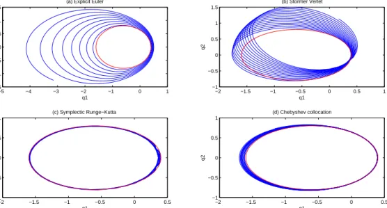
Figure 1 shows some numerical solutions for the eccentricity e= 0.6 compared to the analytic solution. Neither the explicit Euler method nor the Chebyshev collocation method are symplectic, and the phase volume is not preserved, as evidenced by the fact that the associated orbits spiral outwards. However, the Chebyshev collocation method is of higher order than the explicit Euler method, and one observes that the numerical orbit is much more accurate even though the explicit Euler method is advanced using time-steps that are a factor of 100 smaller. The St¨ormer–Verlet method and symplectic Runge–Kutta method are both symplectic, and they both preserve the area of the elliptical orbit.
−5 −4 −3 −2 −1 0 1 −1.5 −1 −0.5 0 0.5 1 1.5
(a) Explicit Euler
q1 q2 −2 −1.5 −1 −0.5 0 0.5 1 −1 −0.5 0 0.5 1 1.5 (b) Stormer Verlet q1 q2 −2 −1.5 −1 −0.5 0 0.5 −1 −0.5 0 0.5 1 (c) Symplectic Runge−Kutta q1 q2 −2 −1.5 −1 −0.5 0 0.5 −1 −0.5 0 0.5 1 (d) Chebyshev collocation q1 q2
Figure 1: Two-body Kepler problem. Total time T = 100. (a) Explicit Euler, time-steph= 0.0025; (b) St¨ormer–Verlet,
time-step h= 0.1; (c) 6th-order symplectic Runge Kutta, time-step h= 0.25; (d) Chebyshev collocation, 5 collocation
points, time-steph= 0.25.
3. Galerkin spectral variational integrators
In this section, we first recall the implementation of spectral variational integrators which falls within the framework of generalized Galerkin variational integrators that were discussed in [12, 19, 24]. One may refer to [12] for a more in depth description and analysis of spectral variational integrators. As spectral variational integrators and spectral-collocation methods are both determined by the choice of a finite-dimensional interpolation space, it is nature for us to be curious about the relative performance of these two methods when they both utilize the same interpolation points. So, we provide numerical comparisons of spectral variational integrators and spectral-collocation methods which both based on Chebyshev–Gauss–Lobatto interpolation in the end of this section.
3.1. Approximation of the exact discrete Lagrangian
To approximate the trajectory q : [0, T] → Q, we divide the total time interval [0, T] into N
subintervals of equal length h, a discrete curve in Qis defined in terms of piecewise polynomial curves
q : [kh,(k+ 1)h]→Q,k = 0, ..., N −1, that are subordinate to the partitioning of the time interval,
[0, T] =
N−1
[
k=0
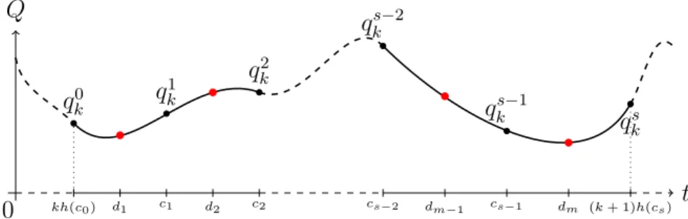
t Q 0 kh(c0) d1 c1 d2 c2 cs−2 dm−1 cs−1 dm (k+ 1)h(cs) q0 k q 1 k q2 k qks−2 qks−1 qsk
Figure 2: The red dots represent the quadrature points, which may or may not be the same as the interpolation points which represented by black dots.
We now discuss how one can systematically approximate the generally non-computable exact discrete Lagrangian LEd(qk, qk+1) with a highly-accurate computable discrete Lagrangian, Ld(qk, qk+1).
Specifi-cally, given a Lagrangian L:T Q→R, we approximate the infinite-dimensional function space,
C([kh,(k+ 1)h], Q) ={q∈C2([kh,(k+ 1)h], Q)|q(kh) = qk, q((k+ 1)h) =qk+1},
that appears in the variational characterization of the exact discrete Lagrangian (7) with a finite-dimensional function subspace,
Cs([kh,(k+ 1)h], Q) = {q ∈ C([kh,(k+ 1)h], Q)|q is a polynomial of degree s}.
As is show in Figure 2, we can consider a discretization of the configuration space on a s-dimensional function space generated by Lagrange interpolating polynomials based on the Chebyshev points cj =
(2k+1)h
2 +
h
2cos(
jπ
s ), where cj are the Chebyshev points xj = cos( jπ
s ),0≤ j ≤s rescaled from [−1,1] to
[kh,(k+ 1)h]. So, for any chosen numerical quadrature formula (wi, τi)mi=1, wherewi are the quadrature weights and τi ∈[−1,1] are the quadrature points, we obtain,
q(di;qvk, h) = s X v=0 qkvlv,s(τ(di)), q˙(di;qkv, h) = s X v=0 qkvlv,s˙ (τ(di))dτ dt = 2 h s X v=0 qkvlv,s˙ (τ(di)),
where τ(t) = 2h(t−tk)−1 ∈ [−1,1], di are the quadrature points in the interval [tk, tk+1], and lv,s(τ)
are the Lagrange basis polynomials of degree s,lv,s(τ) : [−1,1]→R, that are given by lv,s(τ) = Y 0≤j≤s,j6=v τ−xj xv−xj .
Then, we can approximation the discrete Lagrangian as
Ld(qk=qk0, q 1 k, ..., q s k =qk+1;h) = ext q∈Cs([kh,(k+1)h],Q) q0 k=qk,qks=qk+1 h 2 m X i=1 wiL(q(di;qkv, h),q˙(di;qkv, h)) = ext (q0 k,q 1 k,...,q s k) q0 k=qk,qsk=qk+1 h 2 m X i=1 wiL s X v=0 qkvlv,s(τi), 2 h s X v=0 qkvl˙v,s(τi) ! . (25)
3.2. Implementation of multi-interval spectral variational integrators
In (25), requiring that qkv, v = 1, ..., s −1 be stationary points gives the following stationarity conditions, DiLd(qk0, q 1 k, ..., q s k;h) = 0, i= 1, ..., s−1, (26a) Ds+1Ld(qk =qk0, q 1 k, ..., q s k =qk+1;h) +D1Ld(qk+1 =q0k+1, q 1 k+1, ..., q s k+1 =qk+2;h) = 0, (26b)
which can be viewed as a combination of internal stage conditions that can be used to determine
qk1, . . . , qks−1 and the usual the discrete Euler–Lagrange equations. Expanding (26) yields the following set of s+ 1 nonlinear equations,
pk =− m X n=1 wn h 2l0,s(τn) ∂L ∂q Xs v=0 qkvlv,s τn , 2 h s X v=0 qvkl˙v,s τn + ˙l0,s(τn) ∂L ∂q˙ Xs v=0 qkvlv,s τn ,2 h s X v=0 qkvl˙v,s τn , (27a) 0 = − m X n=1 wn h 2lr,s(τn) ∂L ∂q Xs v=0 qkvlv,s τn ,2 h s X v=0 qkvl˙v,s τn + ˙lr,s(τn) ∂L ∂q˙ Xs v=0 qvklv,s τn ,2 h s X v=0 qkvl˙v,s τn , (27b) pk+1 = m X i=n wn h 2ls,s(τn) ∂L ∂q Xs v=0 qvklv,s τn , 2 h s X v=0 qvkl˙v,s τn + ˙ls,s(τn) ∂L ∂q˙ Xs v=0 qvklv,s τn ,2 h s X v=0 qkvl˙v,s τn , (27c) where r= 1, ..., s−1.
Then, (27a) and (27b) can be written in the following matrix form, ˜
AkQ˜k =Gk, (28)
where ˜Ak is a s×(s+ 1) matrix and the entries are given by
˜ Ai,jk = 2 h m X n=1 wnl˙i−1,s(τn) ˙lj−1,s(τn), (29) ˜
Qk is a (s+ 1)-dimensional column vector,
˜ Qk = [qk0, q 1 k, ..., q s k] T,
Gk is a s-dimensional column vector,
Gk = [g0k, g 1 k, ..., g s−1 k ] T = " h 2 m X n=1 wil0,s(τn)· ∂L ∂q, h 2 m X n=1 wil1,s(τn)· ∂L ∂q, ..., h 2 m X n=1 wils−1,s(τn)· ∂L ∂q #T .
As the initial valueqk0can be obtained from the previous step, by considering the partitions ˜Ak = [A1k, Ak] and ˜Qk = [qk0, Qk]T where A1k is the first column of the matrix ˜Ak, we can rewrite (28) to obtain
Then, (30) can be solved using a nonlinear root finder. This gives us the solution ˜Qk. Substituting this into (27c), we can get pk+1. The multi-interval algorithm can be obtained by cycling through the
following diagram, (qk, pk) (27a)(27b) //// Q= (q1 k, qk2, ..., qsk) (27c) //// (qk+1, pk+1) k←k+1 j j
and the iterative algorithm can be summarized as follows:
Table 5: The iterative algorithm of SVI
STEP1. choose the number of collocation points s+ 1 and quadrature formula (wi, τi)mi=1.
STEP2. compute matrix Ak, k = 0, ..., N −1.
STEP3. choose an initial guess for the solution at the collocation pointsQk = (qk1, q2k, ..., qks).
STEP4. compute Gk( ˜Q) and its Jacobian.
STEP5. update Qk = (q1k, qk2, ..., qks) by performing a nonlinear rootfinding iteration for (30),
until max(kQi+1−QikL∞,kP
i+1−Pik
L∞)< T OL. STEP6. letq0
k+1 =qsk and compute pk+1 by (27c).
STEP7. k ←k+ 1, repeat STEP3 to STEP6 .
3.3. Numerical comparisons
In this section, we simulate some classical Hamiltonian systems to explore the relative performance characteristics of the numerical schemes described above. In particular, we compare the spectral vari-ational integrator (SVI) to the spectral-collocation (SC) method and some higher-order symplectic Runge–Kutta (SRK) methods that are derived from the Gauss collocation methods. The properties that we consider in the numerical experiments include the trajectory in phase space, the trajectory in configuration space, momentum, energy behavior and computational time. In the nonlinear solves that are used when implementing the SVI, SC and SRK, we also compare the maximum pointwise errors,
max(kQi+1−QikL∞,kP
i+1−Pik L∞)
and set the tolerance to 10−14 and the maximum iteration count is set to 1000.
3.3.1. Simple harmonic oscillator
The simplest example of an oscillating system is a mass connected to a rigid foundation by a linear spring. This is described by the Lagrangian,
L=T −V = mq˙
2
2 −
kq2
2 , or equivalently with the Hamiltonian,
H =T +V = p
2
2m + kq2
2 ,
wherem andk are mass and spring constant, respectively. The Euler–Lagrange equations are given by,
and Hamilton’s equations are given by ˙ q = p m, (31a) ˙ p=−kq. (31b)
Let m = k = 1, and choose the initial value q0 = 0, p0 = 1. We simulate the simple harmonic
oscillator with both the spectral variational integrator (SVI) and the Chebyshev spectral-collocation (SC) method. Figure 3 compares the trajectory in phase space generated by SVI and SC. To more clearly demonstrate the differences in these two phase trajectories, we plot the phase trajectory every 5 timesteps. Figure 4 shows the position error of these two methods. When we use the same time-step and the same number of Chebyshev points, the position error of SC is several orders of magnitude bigger and grows much faster than SVI. In comparison, the position error of the SVI appears to be bounded and remains small. From Figure 5, we can also see that the energy error of SC is also much bigger and grows much faster than SVI. In Figures 6, 7, 8, we compare the configuration error and energy error under both N-refinement and h-refinement, where N represents the number of collocation points and
h represents the time-step. It is clear that the SVI is more accurate than SC both in configuration and energy errors, when using the same number of collocation points and the same time-step.
−1 −0.5 0 0.5 1 −1 −0.8 −0.6 −0.4 −0.2 0 0.2 0.4 0.6 0.8 1 q p SVI EXACT −1 −0.5 0 0.5 1 −1 −0.8 −0.6 −0.4 −0.2 0 0.2 0.4 0.6 0.8 1 q p SC EXACT
Figure 3: Simple harmonic oscillator, comparison of phase trajectory with time-steph= 1, and total time T = 100 for
SVI and SC, both with 9 Chebyshev points.
0 10 20 30 40 50 60 70 80 90 100 −1 −0.8 −0.6 −0.4 −0.2 0 0.2 0.4 0.6 0.8 1x 10 −11 0 10 20 30 40 50 60 70 80 90 100 −1 −0.8 −0.6 −0.4 −0.2 0 0.2 0.4 0.6 0.8 1x 10 −8
Figure 4: Simple harmonic oscillator, comparison of position error with time-steph= 1, and total timeT = 100 for SVI,
0 50 100 150 200 250 300 350 400 450 500 10−16 10−14 10−12 10−10 10−8 10−6 time energy error SC SVI
Figure 5: Simple harmonic oscillator, comparison of energy error with time-step h= 1, and total timeT = 500 for SVI,
SC both with 9 Chebyshev points.
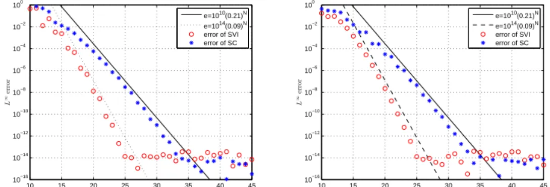
10 15 20 25 30 35 40 45 10−16 10−14 10−12 10−10 10−8 10−6 10−4 10−2 100
Chebyshev Points per step
L ∞ e r r o r e=1010(0.21)N e=1014(0.09)N error of SVI error of SC 10 15 20 25 30 35 40 45 10−16 10−14 10−12 10−10 10−8 10−6 10−4 10−2 100
Chebyshev Points per step
L ∞ e r r o r e=1010(0.21)N e=1014(0.09)N error of SVI error of SC
Figure 6: Simple harmonic oscillator, (left)L∞error ofq over a single time-steph= 20 with N-refinement. (right)L∞
error of energy over a single time-steph= 20 withN-refinement
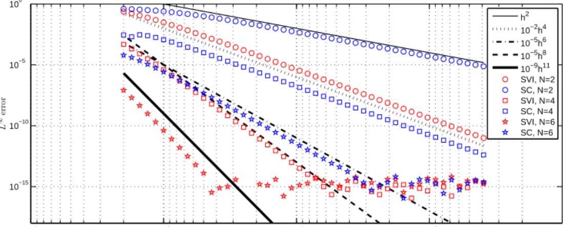
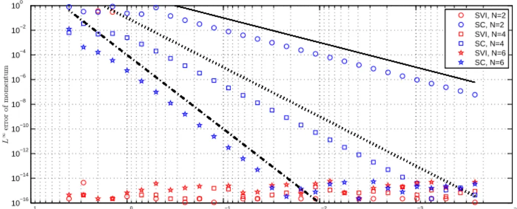
10−3 10−2 10−1 100 101 10−18 10−16 10−14 10−12 10−10 10−8 10−6 10−4 10−2 100 step−size L ∞ e r r o r 1.5h3 10−2h5 10−5h7 10−5h9 10−10h13 SVI, N=2 SC, N=2 SVI, N=4 SC, N=4 SVI, N=6 SC, N=6
Figure 7: Simple harmonic oscillator, L∞ error of q with h-refinement. Here, we use N in the legend to denote the
10−3 10−2 10−1 100 101 10−15 10−10 10−5 100 step−size L ∞ e r r o r h2 10−2h4 10−5h6 10−5h8 10−9h11 SVI, N=2 SC, N=2 SVI, N=4 SC, N=4 SVI, N=6 SC, N=6
Figure 8: Simple harmonic oscillator,L∞error of energy withh-refinement. Here, we useN in the legend to denote the
number of Chebyshev points used to construct the method. 3.3.2. Planar pendulum
The pendulum consists of a mass m attached on a rod of length l. Considering the planar motion in the x-z plane, where the generalized coordinate q ∈ S1 denotes the angle that the rod makes with the direction of gravity. Then, the Lagrangian is given by,
L(q,q˙) = ml
2q˙2
2 +mglcos(q), and the Hamiltonian is given by,
H(q, p) = p
2
2ml2 −mglcos(q).
The corresponding Euler–Lagrange equations are,
ml2q¨+mglsinq= 0,
and Hamilton’s equations are given by ˙
q= p
ml2, (32a)
˙
p=−mglsin(q). (32b)
For simplicity, we assume that m = l = g = 1, and consider the initial conditions q0 = 0.5, p0 = 0.
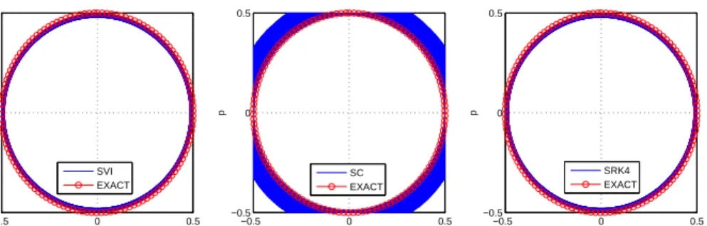
We compare the simulations obtained by SVI, SC, and the 4th-order symplectic Runge–Kutta (SRK) method. Figures 9 and 10 provides a comparison of the trajectories in phase space and the energy error, respectively. We can see that the SVI and SRK, which are both symplectic, preserve the phase area and energy of planar pendulum very well, but a drift is observed in both the phase trajectory and the energy error when using SC, which is consistent with the fact that the method is not symplectic. Table 6 provides a comparison of the computational cost of each method. In particular, we observe that the SVI achieves higher accuracy at a lower computational cost compared to the 4th-order SRK method, and while it costs more than the SC method, it achieves much better long-time accuracy of the phase trajectory and the energy error.
−0.5 0 0.5 −0.5 0 0.5 q p SVI EXACT −0.5 0 0.5 −0.5 0 0.5 q p SC EXACT −0.5 0 0.5 −0.5 0 0.5 q p SRK4 EXACT
Figure 9: Planar pendulum, phase with time-step h= 0.5, and total timeT = 1000 for SVI, SC both with 4 Chebyshev
points and 4th-order symplectic Runge–Kutta method.
0 100 200 300 400 500 600 700 800 900 1000 10−15 10−10 10−5 100 time energy error SC SVI SRK4
Figure 10: Planar pendulum, energy behavior with time-steph= 0.5, and total timeT = 1000 for SVI and SC both with
4 Chebyshev points and 4th-order symplectic Runge–Kutta method.
Table 6: Computational cost of SRK, SVI and SC
SCHEME CPU-TIME STEP-SIZE TOTAL TIME TOL
SRK4 13.73s 0.5 1000 10−14
SVI 4.94s 0.5 1000 10−14
SC 1.85s 0.5 1000 10−14
3.3.3. Duffing oscillator
The Duffing equation is a nonlinear second-order differential equation, which is given by ¨
q+δq˙+αq+βq3 =γcos(ωt)
where the numbers δ, α, β, γ, and ω are prescribed constants. It describes a nonlinear oscillator with damping that is periodically forced, and δ controls the damping,α controls the stiffness, β controls the nonlinearity in the restoring force, γ controls the amplitude of the periodic driving force, andω controls the frequency of the periodic driving force. Since we are concerned with the case where the Duffing equation is Hamiltonian, we consider the undamped and unforced case, where γ =δ = 0. It is easy to check that the Lagrangian is given by L(q,q˙) = 12q˙2 − 1
2αq 2− 1
4βq
4, and the Hamiltonian is given by
H(q, p) = 12p2+ 1 2αq
2 + 1 4βq
4. We compare the spectral variational integrator, Chebyshev collocation
method and 6th-order symplectic Runge–Kutta method, with parameters α=−1, β = 8/3 and initial condition q(0) = 0, ˙q(0) = 1.
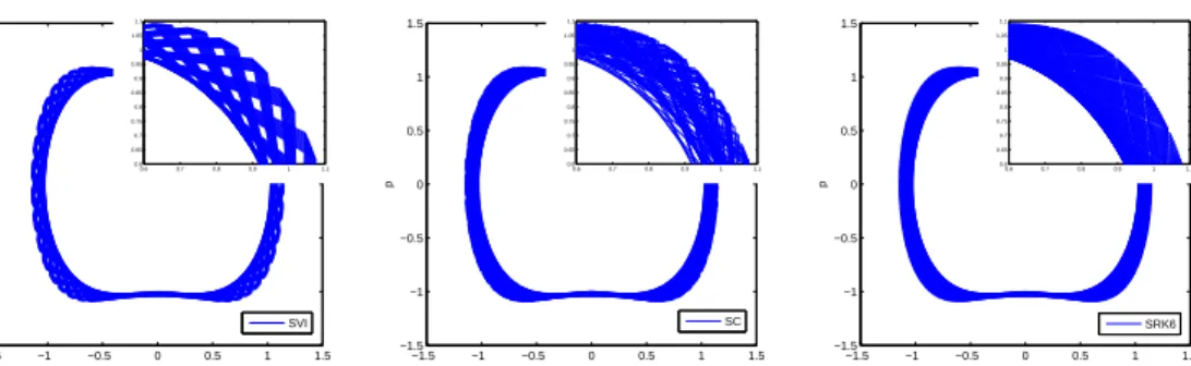
−1.5 −1 −0.5 0 0.5 1 1.5 −1.5 −1 −0.5 0 0.5 1 1.5 q p SVI −1.5 −1 −0.5 0 0.5 1 1.5 −1.5 −1 −0.5 0 0.5 1 1.5 q p SC −1.5 −1 −0.5 0 0.5 1 1.5 −1.5 −1 −0.5 0 0.5 1 1.5 q p SRK6 0.6 0.7 0.8 0.9 1 1.1 0.6 0.65 0.7 0.75 0.8 0.85 0.9 0.95 1 1.05 1.1 0.6 0.7 0.8 0.9 1 1.1 0.6 0.65 0.7 0.75 0.8 0.85 0.9 0.95 1 1.05 1.1 0.6 0.7 0.8 0.9 1 1.1 0.6 0.65 0.7 0.75 0.8 0.85 0.9 0.95 1 1.05 1.1
Figure 11: Duffing oscillator, comparison of phase with time-steph= 0.6, and total timeT = 500 for SVI, SC both with
6 Chebyshev points and 6th-order symplectic Runge–Kutta method.
Figure 11 provides a comparison of the phase trajectory obtained using SVI, SC, and SRK. Under magnification, we see that the phase trajectory of SVI and SRK is very regular, whereas the phase trajectory of SC is much less regular. The energy error is compared in Figure 12, and the computational cost comparison is given in Table 7. We can see that SVI achieves significantly higher-order energy accuracy than SRK while costing less computationally.
0 200 400 600 800 1000 1200 1400 1600 1800 2000 10−14 10−12 10−10 10−8 10−6 10−4 10−2 100 time energy error SC SVI SRK6
Figure 12: Duffing oscillator, comparison of energy behavior with time-step h= 0.6, and total time T = 2000 for SVI,
SC both with 6 Chebyshev points and 6th-order symplectic Runge–Kutta method.
Table 7: Computational cost of SRK, SVI and SC
SCHEME CPU-TIME STEP-SIZE TOTAL TIME TOL
SRK6 86.98s 0.6 2000 10−14
SVI 39.18s 0.6 2000 10−14
SC 4.35s 0.6 2000 10−14
3.3.4. Kepler two-body problem
Now, we compare the spectral variational integrator and Chebyshev collocation method when applied to the Kepler two-body problem. Figures 13, 14, 15 provide a comparison of the orbital trajectory, and the evolution of the energy and momentum. We can see that SVI preserves both energy and momentum very well, while the energy and momentum drift with SC. Figures 16, 17, 18, 19, 20 give a comparison of the error in the configuration, energy, and momentum for Kepler two-body problem underN-refinement and h-refinement. From the error plots, it is not hard to see that SVI is overwhelmingly superior to SC in the accuracy of the trajectory in configuration space, energy and momentum, when using the same number of Chebyshev points and the same time-step. We also find that spectral variational integrators
(27) converge faster and are more stable than spectral-collocation (21), especially with large time-step (See Table 8, Table 9).
−1.5 −1 −0.5 0 0.5 −1 −0.8 −0.6 −0.4 −0.2 0 0.2 0.4 0.6 0.8 1 q1 q2 SVI EXACT −1.5 −1 −0.5 0 0.5 −1 −0.8 −0.6 −0.4 −0.2 0 0.2 0.4 0.6 0.8 1 q1 q2 SC EXACT
Figure 13: Kepler two body, comparison of orbit, with eccentricitye= 0.5, time-steph= 0.2, and total timeT = 2000
for SVI and SC both with 6 Chebyshev points.
0 200 400 600 800 1000 1200 1400 1600 1800 2000 −0.502 −0.501 −0.5 −0.499 −0.498 time energy SC 0 200 400 600 800 1000 1200 1400 1600 1800 2000 −0.5 −0.5 −0.5 −0.5 −0.5 time energy SVI
Figure 14: Kepler two body, comparison of energy, with eccentricitye= 0.5, time-steph= 0.2, and total timeT = 2000
for SVI and SC both with 6 Chebyshev points.
0 200 400 600 800 1000 1200 1400 1600 1800 2000 0.866 0.866 0.866 0.866 0.866 time momentum SVI 0 200 400 600 800 1000 1200 1400 1600 1800 2000 0.8656 0.8658 0.866 0.8662 0.8664 time momentum SC
Figure 15: Kepler two body, comparison of momentum, with eccentricity e = 0.5, time-step h = 0.2, and total time
10 15 20 10−16 10−14 10−12 10−10 10−8 10−6 10−4 10−2 100
Chebyshev Points per step (N)
L ∞ e r r o r o f q1 10 15 20 10−16 10−14 10−12 10−10 10−8 10−6 10−4 10−2 100
Chebyshev Points per step (N)
L ∞ e r r o r o f q2 1070.1N 10100.03N SVI SC 1070.1N 10100.03N SVI SC
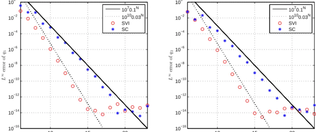
Figure 16: Kepler two body,L∞ error ofq1 andq2over single step h= 5 with N-refinement
10 15 20 10−16 10−14 10−12 10−10 10−8 10−6 10−4 10−2 100
Chebyshev Points per step (N)
L ∞ er ro r o f m o m en tu m 10 15 20 10−16 10−14 10−12 10−10 10−8 10−6 10−4 10−2 100
Chebyshev Points per step (N)
L ∞ er ro r o f en er g y 106(0.1)N SVI SC 106(0.1)N 1013(0.004)N SVI SC
Figure 17: Kepler two body,L∞error of momentum and energy over single steph= 5 withN-refinement
10−4 10−3 10−2 10−1 100 101 10−16 10−14 10−12 10−10 10−8 10−6 10−4 10−2 100 step−size L ∞ e r ro r o f q 1 10−4 10−3 10−2 10−1 100 101 10−18 10−16 10−14 10−12 10−10 10−8 10−6 10−4 10−2 100 step−size L ∞ e r ro r o f q2 1.5h2 10−2 h4 10−5 h6 10−4h8 10−8 h12 SVI,N=2 SC,N=2 SVI,N=4 SC,N=4 SVI,N=6 SC,N=6 1.5h3 10−2 h5 10−5 h7 10−7h10 SVI,N=2 SC,N=2 SVI,N=4 SC,N=4 SVI,N=6 SC,N=6
Figure 18: Kepler two body,L∞error ofq1andq2withh-refinement. Here, we useN in the legend to denote the number
10−4 10−3 10−2 10−1 100 101 10−16 10−14 10−12 10−10 10−8 10−6 10−4 10−2 100 step−size L ∞ e r r o r o f m o m e n t u m SVI, N=2 SC, N=2 SVI, N=4 SC, N=4 SVI, N=6 SC, N=6
Figure 19: Kepler two body, L∞ error of momentum with h-refinement. Here, we use N in the legend to denote the
number of Chebyshev points used to construct the method.
10−4 10−3 10−2 10−1 100 101 10−16 10−14 10−12 10−10 10−8 10−6 10−4 10−2 100 step−size L ∞ er ro r o f en er g y SVI, N=2 SC, N=2 SVI, N=4 SC, N=4 SVI, N=6 SC, N=6
Figure 20: Kepler two body,L∞ error of energy withh-refinement. Here, we useN in the legend to denote the number
of Chebyshev points used to construct the method.
N 2 5 10 15 20
SCHEME SC SVI SC SVI SC SVI SC SVI SC SVI
ITERATION max total max total max total max total max total max total max total max total max total max total
h 0.5 - - 10 1520 8 1271 7 1168 7 1176 7 1176 7 1181 7 1181 7 1186 7 1185 1 - - - - 11 870 9 735 9 709 8 695 8 696 8 695 8 697 8 697 2 - - - - 37 739 11 485 11 476 10 416 10 451 10 414 10 425 10 417 5 - - - 15 279 18 311 14 240 14 261 17 239 8 - - - 23 225 135 536 29 215
Table 8: Kepler problem, number of iterations with eccentricitye=0.2.
4. Shooting-based variational integrators from spectral-collocation methods
Spectral-collocation methods are well-known for their higher accuracy and exponential rates of convergence. Variational integrators are noted for their structure-preserving properties. Our aim in this section is to construct a spectral-collocation variational integrator (SCVI) that combines the benefits of these two numerical methods. To be specific, we discuss how one can construct a variational integrator
N 2 5 10 15 20
SCHEME SC SVI SC SVI SC SVI SC SVI SC SVI
ITERATION max total max total max total max total max total max total max total max total max total max total
h
0.5 - - - - 13 1511 10 1303 9 1277 9 1270 9 1271 9 1271 9 1274 9 1274
1 - - - 14 834 13 815 11 764 11 771 11 760 11 765 11 762
2 - - - 19 674 - - 14 504 17 535 13 481 14 504 18 492
5 - - - 15 279 - - 65 433 - - 114 607
Table 9: Kepler problem, number of iterations with eccentricitye=0.5.
that is based on a spectral-collocation method, that will achieve geometric rates of convergence under
N refinement. It should be noted that in this paper we will restrict our attention to configuration spaces
Qthat are vector spaces. A generalization of spectral-collocation variational integrators for mechanical system on Lie groups will be described in our later work.
4.1. Outline of approach
The proposed approach is based on constructing an approximation of the exact discrete Lagrangian given in (6), where it is expressed in terms of the action integral evaluated on the solution of the Euler– Lagrange boundary-value problem. This was the approached taken in the shooting-based variational integrator that was introduced in [20], but in order to get high order of accuracy, one needed to have numerous quadrature points, and since this approach did not assume that the one-step method used to construct the variational integrator provided access to a piecewise continuous approximation of the solution in the interior of the timestep, the approximations at the quadrature points were obtained by repeatedly applying the underlying one-step method.
In this section, we use the fact that a spectral-collocation method also provides a continuous approx-imation of the solution in the interior of the timestep, so we can use that to construct our computable discrete Lagrangian, and thereby reduce the computational burden of constructing higher-order varia-tional integrators.
4.2. Construction of spectral-collocation variational integrators 4.2.1. Spectral-collocation discrete Lagrangian
Given spectral-collocation method Ψ(hs) :T Q→T Qand a numerical quadrature formula (wi, τi)mi=1, where wi are the quadrature weights and τi ∈ [−1,1] are the quadrature nodes, we can construct the
spectral-collocation discrete Lagrangian as follows
Ld(qk, qk+1;h) = h 2 m X i=1 wiL s X v=0 qvklv,s(τi), 2 h s X v=0 qkvl˙v,s(τi) ! . (33)
where qvk, v = 1, ..., s are obtained from the given spectral-collocation solution of the Euler–Lagrange boundary-value problem. The spectral-collocation solution of the Euler–Lagrange boundary-value prob-lem is defined in two stages, we first solve for the ˜vk that satisfies πQ◦Φ
(s)
h (qk,˜vk) =qk+1, then the qkv, v = 1, ..., sare chosen so Ps
v=0q
v
klv,s(t) is consistent with the initial condition (qk,vk˜ ) and satisfies the
Euler–Lagrange second-order differential equation at the collocation points.
4.2.2. Order of accuracy of the spectral-collocation discrete Lagrangian
For mechanical systems, the Euler–Lagrange equation is generally a second-order nonlinear differen-tial equation, and it is a standard result in the numerical analysis of the shooting method for nonlinear problems [15] that the approximation error in the solution of a boundary-value problem is bounded by the sum of two terms:
(i) the global error of the spectral-collocation method applied to the initial-value problem; (ii) the error associated with the rate of convergence of the nonlinear solver.
The order analysis of the shooting-based discrete Lagrangian depends mainly on the global approxi-mation properties of the shooting solution of two-point boundary-value problems and the accuracy of the quadrature formula. The analysis of h refinement for shooting-based variational integrators was developed in Theorem 1 of [20], which we state here.
Theorem 4.1. (Theorem 1 of [20]) Given a p-th order accurate one-step method Ψ, a q-th order
accurate quadrature formula, and a Lagrangian L that is Lipschitz continuous in both variables, the
associated shooting-based discrete Lagrangian has order of accuracy min(p, q).
This, together with Theorem 2.3.1 of [24], which is the basis of variational error analysis, estab-lishes that the order of accuracy of the variational integrator generated by a shooting-based discrete Lagrangian is min(p, q).
4.2.3. Geometric convergence of the spectral-collocation discrete Lagrangian
We now prove that the shooting-based variational integrator based on spectral-collocation is geo-metrically convergent. We first cite Theorem 3.2 of [12] which extends variational error analysis to the case of geometric convergence of variational integrators.
Theorem 4.2. (Theorem 3.2 of [12])Given a regular LagrangianL and corresponding Hamiltonian
H, the following are equivalent for a discrete Lagrangian L(dN)(q0, q1):
(1) there exist a positive constant K, where K < 1, such that the discrete Hamiltonian map for
L(dN)(q0, qh) has error O(Ks),
(2) there exists a positive constant K, where K < 1, such that the discrete Legendre transforms of
L(dN)(q0, qh) have error O(Ks),
(3) there exists a positive constant K, where K < 1, such that Ld(N)(q0, qh) approximates the exact
discrete Lagrangian LEd(q0, qh, h) with error O(Ks).
With this result in mind, we state a theorem about the extent to which a spectral-collocation discrete Lagrangian approximates the exact discrete Lagrangian.
Theorem 4.3. Given a sequence of spectral-collocation methods Ψ(hN) with error bounded byCAKAN,
for some constants CA, KA < 1 that are independent of N, a sequence of quadrature rules GN(f) =
PmN
j=1bjNf(cjNh) ≈
Rh
0 f(t)dt, such that the quadrature error is bounded by CgK
N
g , for some constants
Cg, Kg <1that are independent ofN, and a LagrangianLthat is Lipschitz continuous in both variables,
the associated spectral-collocation discrete Lagrangian L(dN) has an error bounded by CKN for some
constants C, K <1 that are independent of N.
Proof. A converged shooting solution (˜qk,k+1,v˜k,k+1), associated with a geometrically convergent
spectral-collocation method Ψ(hN), approximates the exact solution (qk,k+1, vk,k+1) of the Euler–Lagrange
boundary-value problem with the following global error:
If the numerical quadrature formula is geometrically convergent, then kLEd(qk, qk+1)−L (N) d (qk, qk+1)k = Z (k+1)h kh L(qk,k+1(t), vk,k+1(t))dt− h 2 m X i=1 wiL(qk,k+1(di), vk,k+1(di)) + h 2 m X i=1 wiL(qk,k+1(di), vk,k+1(di))− h 2 m X i=1 wiL(˜qk,k+1(di),v˜k,k+1(di)) ≤ Z (k+1)h kh L(qk,k+1(t), vk,k+1(t))dt− h 2 m X i=1 wiL(qk,k+1(di), vk,k+1(di)) + h 2 m X i=1 wiL(qk,k+1(di), vk,k+1(di))− h 2 m X i=1 wiL(˜qk,k+1(di),v˜k,k+1(di)) ≤CgKgN + h 2 m X i=1 wi L(qk,k+1(di), vk,k+1(di))−L(˜qk,k+1(di),v˜k,k+1(di)) ≤CgKgN + h 2 m X i=1 wiKLCAKAN =CgKgN +hKLCAKAN ≤(Cg+hKLCA)KN
whereK = max(Kg, KA), and we used the quadrature error, consistency of the quadrature rule, the error estimates on the shooting solution, and the assumption that L is Lipschitz continuous with Lipschitz constant KL.
While we have primarily discussed numerical quadrature formulas that only depend on the integrand, one could consider more general quadrature formulas that depend on derivatives of the integrand, such as Gauss–Hermite quadrature. As to the finite-dimensional function space, we can also consider trigonometric polynomials, wavelets, etc. Different combinations of quadrature formulas and finite-dimensional function spaces may led to effective integrators for specific classes of problems.
4.2.4. Implementation issues of multi-interval schemes
In this section, we describe the numerical implementation of a spectral-collocation variational in-tegrator for mechanical systems with Lagrangian L. In practice, we combine the implicit discrete Euler–Lagrange equations
together with the spectral-collocation method (18) to yield a set of nonlinear equations, A2⊗Imvec(Q) = vec(F(Q, AQ+a0qk0))−a0⊗(vk0) T −(Aa 0)⊗(qk0) T, (34a) qk0 =qk, (34b) qks =qk0+1 =qk+1, (34c) pk =− m X i=1 wi h 2l0,s(τi) ∂L ∂q Xs v=0 qkvlv,s τi , 2 h s X v=0 qvkl˙v,s τi + ˙l0,s(τi) ∂L ∂q˙ Xs v=0 qkvlv,s τi , 2 h s X v=0 qvkl˙v,s τi , (34d) pk+1 = m X i=1 wi h 2ls,s(τi) ∂L ∂q Xs v=0 qkvlv,s τi ,2 h s X v=0 qkvl˙v,s τi + ˙ls,s(τi) ∂L ∂q˙ Xs v=0 qvklv,s τi ,2 h s X v=0 qkvl˙v,s τi , (34e) whereQ= (qk1, qk2, ..., qks). Given an initial condition (qk, pk), we can obtain Q= (q1k, q
2
k, ..., q s
k) by solving
equations (34a) (34b) (34d) with a nonlinear root finder, such as the Newton method, then (qk+1, pk+1)
can be obtained from (34c) (34e). This procedure is summarized in the diagram below, (qk, pk) (34a)(34b)(34d) //// Q= (qk1, qk2, ..., qsk) (34c)(34e) ////(qk+1, pk+1) k←k+1 j j
and the iterative algorithm can be described as follows,
Table 10: The iterative algorithm of SCVI
STEP1. choose the number of collocation points s+ 1 and quadrature formula (wi, τi)mi=1.
STEP2. compute matrix A.
STEP3. choose initial guess of the collocation pointsQ= (q1
k, q2k, ..., qsk) andv0k, a good initial
guess for vk0 can be obtained by inverting the continuous Legendre transformation
p=∂L/∂v.
STEP4. compute the right hand side of (34a),(34d) and their Jacobians.
STEP5. updateQ= (qk1, qk2, ..., qsk) and vk0 by performing a nonlinear rootfinding iteration for (34a),(34d), until max(kQi+1−Qik
L∞,kP
i+1−Pik
L∞)< T OL. STEP6. compute (qk+1, pk+1) by (34c) and (34e).
STEP7. k ←k+ 1, repeat STEP3 to STEP6.
in terms of the generalized coordinates and momenta (q, p) on the cotangent bundle T∗Q, A2⊗Imvec(Q) = vec(F(Q, AQ+a0qk0))−a0⊗(vk0) T −(Aa 0)⊗(qk0) T, (35a) qk0 =qk, (35b) qk0+1 =qk+1, (35c) pk =− m X i=1 wi − h 2l0,s(τi) ∂L ∂q Xs v=0 qkvlv,s τi , pi +pil˙0,s(τi) , (35d) pk+1 = m X i=1 bi −h 2ls,s(τi) ∂L ∂q Xs v=0 qkvlv,s τi , pi +pil˙s,s(τi) , (35e) ∂L ∂p Xs v=0 qvklv,s τi , pj − 2 h s X v=0 qkvl˙v,s(τi) = 0, j = 1, ..., m. (35f) 4.3. Numerical examples
In this part, we explicitly derive the numerical method for the proposed spectral-collocation varia-tional integrator (SCVI) in the case of 2 interpolation points and 2 quadrature points. To verify the effectiveness of the SCVI numerical scheme, we compute the solution of planar pendulum and Kepler two-body problem. In the nonlinear solves used to implement the SCVI, we compare the maximum pointwise errors,
max(kQi+1−QikL∞,kP
i+1−Pik L∞)
and set the tolerance to 10−12 and the maximum iteration count is set to 1000.
4.3.1. Planar pendulum
Consider the ideal model of a planar pendulum (32). For simplicity, we let the massm = 1, massless rod length l= 1 and gravitational acceleration g = 1. Then, the Lagrangian is given by,
L(q,q˙) = ml 2q˙2 2 +mglcos(q) = ˙ q2 2 + cos(q), The corresponding Euler-Lagrange equation is,
¨
q+ sinq= 0.
Here, we choose two Chebyshev points x0 =−1, x1 = 1 and the two-point Gauss quadrature formula
(wi, τi)2i=1 where
w=±1; τ =±√1
3.
Then, the approximation of q at the corresponding rescaled quadrature points in the interval [kh,(k+ 1)h] is given by, q(d1) =l0,1 −√1 3 qk+l1,1 −√1 3 qk+1 = 3 +√3 6 qk+ 3−√3 6 qk+1. q(d2) =l0,1 1 √ 3 qk+l1,1 1 √ 3 qk+1 = 3−√3 6 qk+ 3 +√3 6 qk+1.
From (11), we can obtain the first-order Chebyshev differential matrix in the interval [−1,1] based on Chebyshev points x0 =−1, x1 = 1, D(1) = 1 2 − 1 2 1 2 − 1 2
Then, the first-order Chebyshev differential matrix in the interval [kh,(k+ 1)h] can be given by, ˜ A=−2 hD (1)(2 : 2,1 : 2) = − 1 h, 1 h .
We can partition the 1×2 matrix ˜A into ˜A= [a0, A]. Combined with (34b), (34a) has the form,
1 h2qk+1 =−sin(qk+1)− −1 h vk− − 1 h2 qk, (36)
and (34d) can be calculated by using (30), where ˜ Ak = [A1k, Ak] = 2 h 2 X n=1 wnl˙0,1(τn) ˙l0,1(τn), 2 h 2 X n=1 wnl˙0,1(τn) ˙l1,1(τn) = 1 h,− 1 h , Gk = h 2 2 X n=1 wnl0,1(τn) −sin l0,1(τn)qk+l1,1(τn)qk+1 =−(3 + √ 3)h 12 sin 3 +√3 6 qk+ 3−√3 6 qk+1 ! − (3− √ 3)h 12 sin 3−√3 6 qk+ 3 +√3 6 qk+1 ! .
From this, (34d) can be rewritten as,
Akqk+1+A1kqk+Gk+pk = 0. (37)
So, we can solve for vk and qk+1 using (36) and (37). Then, we can calculate pk+1 from (34e).
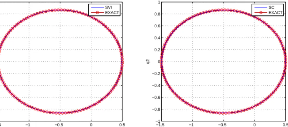
Choosing the initial valueq0 = 0.5, p0 = 0, Figure 21 shows the phase trajectories of the pendulum
system, which are computed using the two-point spectral-collocation variational integrator (SCVI) constructed above, and the Chebyshev collocation (SC) method, also with 2 collocation points. Figure 22 shows the corresponding energy errors of these two methods. From the numerical results, we can see that SCVI preserves the phase space area and energy very well, as one would expect from a symplectic integrator, whereas the Chebyshev collocation method performs much more poorly in terms of preserving the phase area and energy. In particular, the Chebyshev collocation method exhibits a decay of the trajectory in phase space.
−0.5 0 0.5 −0.5 −0.4 −0.3 −0.2 −0.1 0 0.1 0.2 0.3 0.4 0.5 q p SCVI EXACT −0.5 0 0.5 −0.5 −0.4 −0.3 −0.2 −0.1 0 0.1 0.2 0.3 0.4 0.5 q p SC EXACT
Figure 21: Planar pendulum. Comparison of phase trajectories. Left figure: time-step h= 0.005, 2 collocation points,
2 quadrature points, and total time T = 60π; Right figure: time-step h = 0.005, 2 collocation points, and total time
T = 60π. 0 20 40 60 80 100 120 140 160 180 10−10 10−8 10−6 10−4 10−2 100 time energy SC SCVI
Figure 22: Comparison of energy of planar pendulum problem computed using SCVI with 2 collocation points, 2
quadra-ture points and SC with 2 collocation points. Time-steph= 0.005.
4.3.2. Kepler two-body problem
We test the SCVI numerical method (34) on the Kepler problem which has already been described in Section 3.2. The system has not only the total energy H(q, p) as a first integral, but also the angular momentum M(q1, q2, p1, p2) =q1p2−q2p1. For the system (24) we choose, with e= 0.5, the initial value
q1(0) = 0.5, q2(0) = 0, v1(0) = 0, v2(0) =
√
3.
This implies that H0 = −0.5, and M0 =
p
3/4. Figure 23 shows the orbit of Kepler problem when using SCVI with 2 collocation points. We run the numerical program for 10000 periods. In order to maintain the visibility of the trajectory in the figure, we plot trajectory segments from the beginning, middle, and end of the full trajectory.
−1.5 −1 −0.5 0 0.5 1 1.5 −1.5 −1 −0.5 0 0.5 1 1.5 step 1 to 2150 q1 q2 −1.5 −1 −0.5 0 0.5 1 1.5 −1.5 −1 −0.5 0 0.5 1 1.5 step 198925 to 201075 q1 q2 −1.5 −1 −0.5 0 0.5 1 1.5 −1.5 −1 −0.5 0 0.5 1 1.5 step 397850 to 400000 q1 q2
Figure 23: Orbit of Kepler problem computed using SCVI with 2 collocation points. Time-steph=π/20, and total time
T = 20000π.
In Figure 24, 25, 26, we compare the orbit, momentum and energy of the Kepler problem, when simulated using SCVI with 2 collocation points and Chebyshev collocation method with 3 collocation points (the two-point Chebyshev collocation method is not stable when we set the time-step h = 0.1). In the left column of Figure 24, we show the comparison of the orbit over 30 periods and in the right column of Figure 24, the orbit of the last period are given. The column of subfigures on the right show the last part of the trajectory, over one orbital period of the exact solution. It is clear that the period of the system does not change when using the SCVI method, but the orbital period shrinks by a factor of almost three when using the Chebyshev collocation method.
−1.5 −1 −0.5 0 0.5 1 −1.5 −1 −0.5 0 0.5 1 q1 q2 SCVI EXACT −1.5 −1 −0.5 0 0.5 1 −1.5 −1 −0.5 0 0.5 1 q1 q2 SCVI EXACT −1.5 −1 −0.5 0 0.5 1 −1 −0.5 0 0.5 1 q1 q2 SC EXACT −1.5 −1 −0.5 0 0.5 1 −1 −0.5 0 0.5 1 q1 q2 SC EXACT
Figure 24: Kepler problem. Comparison of orbit computed using SCVI with 2 collocation points and SC with 3 collocation
points. Time-steph= 0.1, and total timeT = 60π. The second column of figures show the last part of the trajectory for
0 5 10 15 20 25 30 0.65 0.7 0.75 0.8 0.85 0.9 Comparison of momentum t momentum SC SCVI
Figure 25: Kepler problem. Comparison of momentum computed using SCVI with 2 collocation points and SC with 3
collocation points. Time-steph= 0.1, and total timeT = 60π.
0 5 10 15 20 25 30 −2.5 −2 −1.5 −1 −0.5 0 0.5 1 1.5 2 Comparison of energy t energy SC total energy SC kinematic SC potential SCVI total energy SCVI kinematic SCVI potential
Figure 26: Kepler problem. Comparison of energy computed using SCVI with 2 collocation points and SC with 3
collocation points. Time-steph= 0.1, and total timeT = 60π.
Figure 27 shows the phase trajectories of the Kepler problem computed using different numerical methods including a symplectic Runge–Kutta method, a spectral-collocation variational integrator, St¨ormer–Verlet and a Chebyshev collocation method. Here, we set the time-step h = 0.3 for the symplectic Runge-Kutta method, spectral-collocation variational integrator, and Chebyshev collocation method. The time-step for St¨ormer–Verlet ish= 0.15. As is show, all the methods we used preserve the area of phase space well, except for the Chebyshev collocation method, which is the only non-symplectic integrator considered here.
−2 −1.5 −1 −0.5 0 0.5 1 1.5 −1.5 −1 −0.5 0 0.5 1 1.5 2 (a) SRK4 q p −2 −1.5 −1 −0.5 0 0.5 1 1.5 −1.5 −1 −0.5 0 0.5 1 1.5 2
(b) SCVI with 4 collocation points
q p −2 −1.5 −1 −0.5 0 0.5 1 1.5 −1.5 −1 −0.5 0 0.5 1 1.5 2 (c) Stormer Verlet q p −2 −1.5 −1 −0.5 0 0.5 1 1.5 −1.5 −1 −0.5 0 0.5 1 1.5 2
(d) SC with 4 collocation points
q
p
Figure 27: Phase trajectories for the Kepler two-body problem.
Figure 28 presents a comparison of the orbits computed using SCVI with 9 Chebyshev points and 5, 6, 7 Gauss quadrature points, from left to right. Figures 29 and 30 present the corresponding momentum and energy behaviors. From the numerical results, we see that SCVI preserves the phase area and momentum, and the energy error remains bounded. It should be noted that the leftmost subfigure corresponding to 5 collocation points is exhibiting precession, which is why the total trajectory sweeps out an annulus. The accuracy of SCVI is determined by both the choice of collocation points and quadrature points. If we fix the number of Chebyshev points, the SCVI achieves higher-order accuracy as we increase the number of quadrature points, at least until the quadrature rule is sufficiently accurate to resolve the action integral sufficiently.
−1.5 −1 −0.5 0 0.5 1 1.5 −1.5 −1 −0.5 0 0.5 1 1.5 q1 q2 SCVI_C9G5 EXACT −1.5 −1 −0.5 0 0.5 −1 −0.8 −0.6 −0.4 −0.2 0 0.2 0.4 0.6 0.8 1 q1 q2 SCVI_C9G6 EXACT −1.5 −1 −0.5 0 0.5 −1 −0.8 −0.6 −0.4 −0.2 0 0.2 0.4 0.6 0.8 1 q1 q2 SCVI_C9G7 EXACT
Figure 28: Two-body Kepler problem. Time-step h= 0.3, and total time T = 400π. Comparison of orbit of
0 50 100 150 200 10−3 10−2 10−1 period momentum SCVI_C9G5 0 50 100 150 200 10−15 10−10 10−5 100 period momentum SCVI_C9G6 0 50 100 150 200 10−10 10−8 10−6 10−4 period momentum SCVI_C9G7
Figure 29: Two-body Kepler problem.Time-step h = 0.3, and total time T = 400π. Comparison of momentum of
spectral-collocation variational integrator (SCVI) with 9 collocation points, 5, 6, 7 quadrature points (from left to right).
0 50 100 150 200 10−1.9 10−1.7 10−1.5 period energy SCVI_C9G5 0 50 100 150 200 10−7 10−6 10−5 10−4 10−3 period energy SCVI_C9G6 0 50 100 150 200 10−8 10−7 10−6 10−5 10−4 period energy SCVI_C9G7
Figure 30: Two-body Kepler problem. Time-step h = 0.3, and total time T = 400π. Comparison of energy error of
spectral-collocation variational integrator (SCVI) with 9 collocation points, 5, 6, 7 quadrature points (from left to right).
5. Conclusions and future directions
In this paper, we present two general techniques for constructing variational integrators that are spectrally accurate. One is based on a Galerkin construction and the other is based on using the spectral-collocation method to solve the Euler–Lagrange boundary-value problem. Methods based on these two approaches are tested on several classical Hamiltonian systems, and their performance relative to other methods is studied through a series of numerical experiments.
From the comparison of Galerkin spectral variational integrators and spectral-collocation methods, we observe the following:
(i) Galerkin spectral variational integrators partially inherit the computational efficiency of spectral methods and show better stability property than Chebyshev collocation methods when using large time-steps, and compare very favorably to symplectic Runge–Kutta methods in terms of computational efficiency.
(ii) Galerkin spectral variational integrator is more accurate in phase, momentum and energy than Chebyshev collocation method when choosing the same number of collocation points and the same time-step.
(iii) Both Galerkin spectral variational integrators and symplectic Runge–Kutta methods are phase and momentum preserving and exhibit good long-term energy stability. In contrast, drifts in the phase and momentum are observed when using the Chebyshev collocation method.
Additionally, we provide a general method to convert any spectral-collocation method to its corre-sponding shooting-based variational integrator, where the existing techniques from approximation the-ory, numerical quadrature, and the spectral method are combined systematically. Another important aspect is the manner in which vectorization of the numerical method allows one to efficiently implement the spectral-collocation variational integrator. Numerical experiments demonstrate that the shooting-based variational integrators from spectral-collocation methods are symplectic, momentum-preserving
and exhibit excellent energy behavior. Like its Galerkin spectral variational integrator counterpart, this new numerical method also partially inherits the computational efficiency of the underlying Chebyshev collocation method.
Both classes of spectrally-accurate variational integrators provide compelling options that combine computational efficiency with geometric structure-preservation. Our future work will focus on extending the synthesis of variational integrators and spectral-collocation methods to Hamiltonian PDEs and systems that evolve on Lie groups and homogeneous spaces.
Acknowledgements
The research of YQL was conducted in the mathematics department at University of California, San Diego. YQL was supported by the graduate school of Harbin Institute of technology. ML was supported in part by NSF Grants CMMI-1029445, DMS-1065972, CMMI-1334759, DMS-1345013, DMS-1411792, and NSF CAREER Award DMS-1010687.
References
[1] N. Bou-Rabee and H. Owhadi. Stochastic variational integrators. IMA J. Numer. Anal., 29(2): 421–443, 2009.
[2] N. Bou-Rabee and H. Owhadi. Long-run accuracy of variational integrators in the stochastic context. SIAM J. Numer. Anal., 48(1):278–297, 2010.
[3] W. L. Briggs and V. E. Henson.The DFT: An Owner’s Manual for the Discrete Fourier Transform. Society for Industrial and Applied Mathematics (SIAM), Philadelphia, PA, 1995.
[4] J. C. Butcher. Implicit Runge-Kutta processes. Math. Comp., 18:50–64, 1964.
[5] J. C. Butcher. A stability property of implicit Runge–Kutta methods.BIT Numerical Mathematics, 15(4):258–361, 1975.
[6] J. C. Butcher. Numerical methods for ordinary differential equations. John Wiley & Sons, Ltd., Chichester, second edition, 2008.
[7] B. L. Ehle. High order A-stable methods for the numerical solution of systems of D.E.’s. BIT
Numerical Mathematics, 8:276–278, 1968.
[8] A. Farr´es, J. Laskar, S. Blanes, F. Casas, J. Makazaga, and A. Murua. High precision symplectic integrators for the Solar System. Celestial Mech. Dynam. Astronom., 116(2):141–174, 2013. [9] B. Gladman, M. Duncan, and J. Candy. Symplectic integrators for long-term integrations in
celestial mechanics. Celestial Mech. Dynam. Astronom., 52(3):221–240, 1991.
[10] E. Hairer and G. Wanner. Solving ordinary differential equations. II, volume 14 ofSpringer Series
in Computational Mathematics. Springer-Verlag, Berlin, second edition, 1996. Stiff and
[11] E. Hairer, C. Lubich, and G. Wanner. Geometric numerical integration, volume 31 of Springer
Series in Computational Mathematics. Springer-Verlag, Berlin, second edition, 2006.
Structure-preserving algorithms for ordinary differential equations.
[12] J. Hall and M. Leok. Spectral variational integrators. Numerische Mathematik, 130(4):681–740, 2015.
[13] E. R. Johnson and T. D. Murphey. Scalable variational integrators for constrained mechanical systems in generalized coordinates. IEEE Transaction on Robotics, 25(6):1249–1261, 2009.
[14] N. Kanyamee and Z. Zhang. Comparison of a spectral collocation method and symplectic methods for Hamiltonian systems. International Journal of Numerical Analysis and Modeling, 8(1):86–104, 2011.
[15] H. B. Keller. Numerical methods for two-point boundary value problems. Dover Publications, Inc., New York, 1992. Corrected reprint of the 1968 edition.
[16] M. Kobilarov and J. E. Marsden. Discrete geometric optimal control on Lie groups. IEEE
Trans-action on Robotics, 27(4):641–655, 2011.
[17] J. D. Lambert. Numerical methods for ordinary differential systems: The initial value problem. John Wiley & Sons, Ltd., Chichester, 1991.
[18] T. Lee, N. H. McClamroch, and M. Leok. Optimal attitude control for a rigid body with symmetry.
Proc. American Control Conf., pages 1073–1078, 2007.
[19] M. Leok. Generalized Galerkin variational integrators: Lie group, multiscale, and pseudospectral methods. (preprint, arXiv:math.NA/0508360), 2004.
[20] M. Leok and T. Shingel. General techniques for constructing variational integrators. Frontiers of
Mathematics in China, 7(2):273–303, 2012.
[21] M. Leok and T. Shingel. Prolongation-collocation variational integrators. IMA J. Numer. Anal., 32(3):1194–1216, 2012.
[22] A. Lew, J. E. Marsden, M. Ortiz, and M. West. Asynchronous variational integrators. Arch.
Ration. Mech. Anal., 167(2):85–146, 2003.
[23] W. J. Liu, B. Y. Wu, and J. B. Sun. Some numerical algorithms for solving the highly oscillatory second-order initial value problems. Journal of Computation Physics, 276(0):235–251, 2014. [24] J. E. Marsden and M. West. Discrete mechanics and variational integrators. Acta Numer., 10:
357–514, 2001.
[25] J. E. Marsden, S. Pekarsky, and S. Shkoller. Discrete Euler-Poincar´e and Lie-Poisson equations.
Nonlinearity, 12(6):1647–1662, 1999.
[26] S. Ober-Bl¨obaum and N. Saake. Construction and analysis of higher order Galerkin variational integrators. Advances in Computational Mathematics, 2014.