Graph partitioning and scheduling for distributed dataflow computation

(1)

Institute of Parallel and Distributed Systems University of Stuttgart

Universitätsstraße 38 D–70569 Stuttgart

Bachelorarbeit

Graph Partitioning and

Scheduling for Distributed

Dataflow Computation

Larissa Laich

Course of Study: Softwaretechnik

Examiner: Prof. Dr. Kurt Rothermel Supervisor: Dr. Muhammad Adnan Tariq,

Dipl.-Inf. Christian Mayer

Commenced: September 14, 2016 Completed: March 16, 2017

(2)

(3)

Abstract

During the last years, the amount of data which can be represented and processed as graph structured data has massively increased. To process these large data sets, graph processing systems have been developed which distribute and partition a graph among multiple machines. Due to an increase in processing power and data collection, machine learning and especially neural networks have become very popular. Consequently, machine learning systems like TensorFlow have emerged. Machine learning models can be represented as dataflow graphs and often take days to train as the dataflow graph is executed thousands of times. Graph partitioning determines how the graph is divided and which node is placed on which device. Scheduling decides which node should be computed next during execution. Smart partitioning and scheduling can drastically reduce the total execution time. Most existing solutions do not consider serveral important constraints like memory limitations, device or colocation constraints which can be directly derived from the machine learning library TensorFlow. This thesis presents and evaluates different partitioning and scheduling strategies meeting the constraints required for a realistic environment. One of these developed partitioning algorithms is based on a heuristic function considering execution time, memory and traffic and tries to map time-critical nodes on fast devices. This partitioning algorithm performed very well in combination with a scheduling strategy which schedules the executable node first whose upwards path takes longest to compute. On the evaluated graphs extracted from TensorFlow, this strategy was up to 75 % and at least 45% better in terms of graph execution time than the slightly adapted popular HEFT algorithm which is a common benchmark. In combination with the aforementioned scheduling strategy a partitioning which aims to assign the critical path nodes to the fastest device showed equally promising results.

(4)

(5)

List of Figures

1.1 Different scheduling algorithms influence the total execution time on the

same partitioning. . . 12

2.1 The dataflow graph is divided onto three machines . . . 17

2.2 Post-processing to insert send and receive nodes after partitioning . . . . 19

2.3 The graph is divided onto three machines. Each node has a node id (upper value) and number of operations (lower value). The labels on the edges represent the tensor size. . . 20

2.4 Schedule of the sample graph shown in Figure 2.3 . . . 21

3.1 Evaluation framework pipeline and its components . . . 26

3.2 Sample graph labelled with node id, #ops and edge weigths . . . 30

5.1 Scheduling strategies . . . 43

6.1 Size and number of colocation groups . . . 47

7.9 Device utilization for the scheduling and partitioning strategies . . . 59

7.10 Number of executable nodes per device before making the decision which is node is executed next . . . 60

(8)

(9)

List of Tables

2.1 Scheduling order per device . . . 20

2.2 Notation overview . . . 22

7.1 Properties of six synthetic graphs . . . 49

(10)

(11)

1 Introduction

During the last decade the collection of graph structured data as well as the processing power massively increased. Due to these new possibilities distributed graph processing systems like Pregel [MAB+10], PowerGraph [GLG+12], GrapH [MTLR16] or GraphCEP [MMTR16] for large-scale graph computation emerged. A powerful application is the execution of machine learning algorithms which are for example used for natural language processing [CW08] or image classification [KSH12].

Machine learning models often consist of billions of parameters [DCM+12] and can be represented as dataflow graphs. In order to shorten the training and execution time the computation is distributed and therefore the graph is partitioned onto different machines. Moreover, the graph could be too large to fit on a single machine which is another reason for partitioning. Other possibilities to reduce the execution time are model replication [NSB+15], pipelining [AC86] or computing a batch of input data at once [LZCS14] and merge the results. This thesis focuses on the partitioning approach.

A graph can be partitioned by dividing its nodes into disjoint subsets, i.e. cut the edges [CSCC15]. The classic k-way partitioning problem is to divide a graph’s node set in k equal sized subsets in a way that the number of cut edges is minimized. This problem is NP-complete [KK98]. When executing the graph, the node execution order is determined by the scheduling for each device.

Clearly, minimizing the execution time as well as the network traffic is an important challenge. The dataflow graph is executed multiple times and therefore runtime informa-tion can be collected and later used for an improved partiinforma-tioning. Furthermore, it takes much time to execute the model in a similar manner over and over again [CZG+16]. Therefore, one might consider to spend more time on the partitioning and scheduling to reduce the overall execution time.

In order to meet all the from TensorFlow derived criteria for the partitioning of machine learning models the standard graph partitioning problem has to be extended. In par-ticular, constraints like memory, device constraints or heterogenous devices have to be considered when searching for a realistic graph partitioning solution.

However, the partitioning problem has to be investigated in combination with the scheduling problem as a bad scheduling can increase the execution time drastically.

(12)

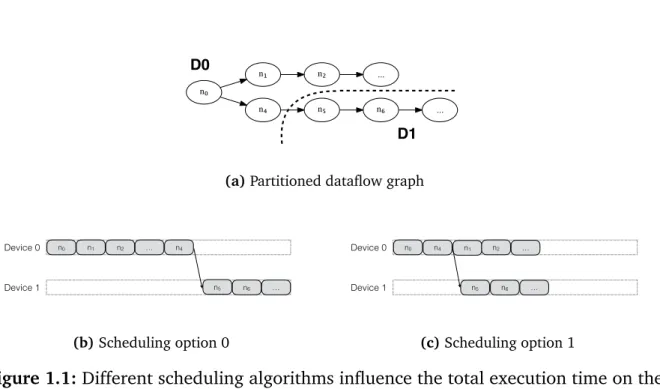
n₀ n₁ n₄ n₂ ... n₅ n₆ ... D0 D1 (a)Partitioned dataflow graph

Device 0 Device 1 n5 n0 n1 n2 … n4 n6 … (b)Scheduling option 0 Device 0 Device 1 n5 n0 n4 n1 n2 … n6 … (c)Scheduling option 1

Figure 1.1: Different scheduling algorithms influence the total execution time on the same partitioning.

Consider the example of Figure 1.1 (a) depicting a dataflow graph which is partitioned onto device 0 and device 1. In Figure 1.1 (b) the scheduling option 0 is visualized in whichn4 is executed only when n1 and all its successors are executed. This becomes

even worse the longer the execution of the direct and indirect successor nodes of n1

takes. Scheduling option 1 which is shown in Figure 1.1 (c) would be a better choice as it enables parallel execution by executing n4 beforen1 and thus shortens the total

execution time.

In this thesis, we developed multiple partitioning and scheduling algorithms considering constraints which are derived from the machine learning library TensorFlow. We compare and evaluate these algorithms which aim to reduce the overall execution time and traffic.

1.1 Contributions

In particular, the thesis provides the following contributions:

1. We defined a system model which contains the constraints derived from the machine learning library TensorFlow. Moreover, the scheduling and partitioning problem was formulated considering the additional constraints.

(13)

1.2 Outline

2. To solve the modified partitioning problem, multiple partitioning strategies were developed. Moreover, three scheduling strategies were implemented.

3. In order to evaluate the aforementioned combinations of scheduling and parti-tioning algorithms an evaluation framework has been developed. The framework is easily extendable and allows a quick integration and implementation of new strategies.

4. We compared partitioning and scheduling algorithms with respect to their execu-tion time and traffic. The results have been visualized.

1.2 Outline

Beyond the introduction chapter this thesis is structured as follows. In Chapter 2 TensorFlow is introduced, the system model is defined and the problem is formulated. Chapter 3 presents an approach to solve the problem and describes multiple components in the developed evaluation pipeline. The scheduling and partitioning problem is described more detailed in Chapter 4 and 5. In these chapters multiple strategies are presented and discussed. In Chapter 6 the generation of sample data is presented. These data sets are used to compare and evaluate the partitioning and scheduling strategies in Chapter 7. Related work is presented in Chapter 8 while future work and drawbacks of the existing solutions are discussed in Chapter 9. The whole thesis is concluded in Chapter 10.

(14)

(15)

2 System Model and Problem

formulation

In the following sections the system model is defined and the problem is formulated. Therefore, the machine learning library TensorFlow and its properties are described in order to derive model properties. Beyond the model, the metrics execution time and traffic are presented which are used to evaluate partitioning and scheduling algorithms in chapter 7. An example illustrates how the execution time is calculated theoretically. For clarity, we reduced the model complexity of TensorFlow as shown in Section 2.6.

2.1 TensorFlow™

The system model and the required constraints are derived from TensorFlow [MAP+15] [ABC+16] [Sca16]. TensorFlow is a machine learning library which was developed by Google and published as open source in November 2015. It has become one of the most popular machine learning libraries since then. TensorFlow is widely used for deep learning models (multi-layer neural networks) and has a C++, python and Java API. In former times many researchers used a machine learning flexible library for research and an efficient one for production. TensorFlow wants to combine both in order to deploy models easily which have been developed during research.

To train a machine learning model in TensorFlow, a computational graph has to be defined and executed. In this case, a computational graph is a stateful dataflow graph. There are implicit data dependencies: A node can not be executed until all predecessor nodes are executed and their computed tensor (multidimensional array) is transferred. Computations make side-effects to variables (model parameters) which are used in future runs and the results of the machine learning. During training, a forward pass [CZG+16] with the current values of the model parameters is calculated. In supervised learning, the result is compared with the true label and an error term is computed. Afterwards, the results are backpropagated and the weights of the model parameters are adjusted.

(16)

2.1.1 Parallelism

Parallelism is an important concept in order to reduce the execution time. In TensorFlow, model as well as data parallelism is possible.

For data parallelism, the model is replicated [NSB+15]. The input data is split and different subsets of the data are trained on the replications of the model. The same global model is updated e.g by taking the parameter average of the model replications. These updates can be performed synchronously or asynchronously. In synchronous data parallelism, the data is divided into batches and computed on x model replicas. After-wards, the gradient is computed and the model is updated synchronously. Alternatively, each replica updates asynchronously. Challenges for data parallelism are for example to tolerate different processing speeds of the model replicas.

For model parallelism, the model is split on different devices [NSB+15] and can be computed in parallel due to the placement on multiple devices. Two nodes can potentially be executed in parallel if they are placed on different devices and there is no data dependency between them.

2.2 Model

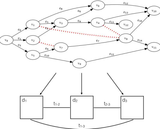
This section defines a system model in which the requirements derived from TensorFlow are considered. Figure 2.1 shows the acyclic dataflow graph which has to be divided on three machines. Each node represents a computation and has a unique id as well as computation or operation costs #ops which represent the necessary number of operations to compute the node’s result. A node can not be executed until all direct predecessor vertices are computed. Furthermore, a vertex has a device constraint (CPU, GPU, TPU or ALL) indicating on which device type the vertex can be executed. TPU stands for Tensor Processing Unit [ABC+16] and is a custom chip developed by Google for machine learning applications. The device condition might reduce the number of feasible devices on which a vertex can be assigned. To store a vertex a defined amount of memory is necessary which is provided in advance.

Each edge represents a tensor being transferred from one vertex to another. An edge has a weight indicating the size of the transferred tensor. If a vertex has multiple outgoing edges all outgoing edges have the same weight and the result is available after the vertex is computed.

In addition to the set of vertices and edges a graph is defined by a set of colocations C. Each colocation constraint contains two nodes which have to be assigned to the same machine. The colocations are represented as red dots in Figure 2.1.

(17)

2.3 Problem Formulation

The graph G has to be divided into n subgraphs and mapped on a set of devices D = {d1, d2, ..., dn}. A device has a device type (CPU, GPU or TPU), memory size and speed which is defined as number of operations per execution unit. Each device can communicate with every other device which is important to be able to transfer tensors. The communication speed between device x and y is defined by a transfer ratetx−y. In our model only one node can be executed by a device at once. Once a node is executed it can not be interrupted as non-preemptive scheduling is assumed.

d1 d2 d3 t1-2 t2-3 t1-3 v₀ v₁ e₀ v₂ e₁ v₅ e₅ v₃ e₃ v₆ e₈ v₈ e₂ v₇ v₄ e₄ e₆ _e_₁₃ v₁₀ v₁₂ e₁₁ e₉ v₉ e₁₀ e₁₂ e₇ e₁₆ v₁₁ e₁₄ e₁₅

Figure 2.1: The dataflow graph is divided onto three machines

2.3 Problem Formulation

In order to fulfil the requirements of the TensorFlow library, the standard partitioning problem has to be adapted to consider multiple constraints.

A graph is defined by G = (V, E, C) in which V = {v0, v1, ..., vr} is a set of vertices,

(18)

tuple (vx, vy)∈C defines two vertices which have to be assigned to the same machine. Bigger colocation groups are formed transitively. In our model the graph is a directed acyclic graph.

The goal of graph partitioning is to split the set of vertices onto n machines. An edge cut divides the graph by assigning vertices to different machines and thereby cutting edges. Scheduling defines the vertex execution order. Both problems are further described in Chapter 4 and 5.

The overall goal is to minimize two factors:

The first and more important one is the execution time or also called makespan. It is defined as the first point of time on which every device has finished computation. This relation is expressed in Equation 2.1. All abbreviations and function names are listed in Table 2.2.

makespan= max

d∈D exec(d) (2.1)

The other metric is the traffic which is defined as the sum of all cross-device edges’ tensor sizes. This is formulated in Equation 2.2.

traffic= X e∈CE

size(e), CE ={(vx, vy, x)∈E∧d(vx)̸=d(vy)} (2.2)

2.4 Insertion of Send and Receive Nodes

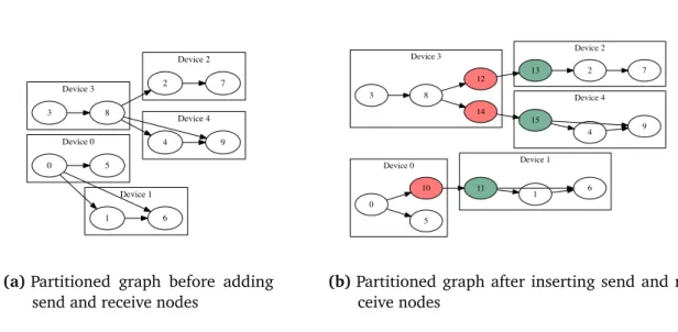
In this section the process of adding send and receive nodes is decribed. After partition-ing, send and receive nodes are inserted for cross-device edges. If a vertex has multiple successor nodes which are assigned to the same machine only one send-receive-node-pair is inserted. This has the huge advantage of transmitting data only once. Furthermore, it also makes a better code abstraction level possible as send and receive nodes can be the only nodes responsible for inter-device data transfer.

Figure 2.2 (a) depicts a dataflow graph which is partitioned onto five devices. After partitioning, the send and receive nodes are inserted. The resulting graph is shown in Figure 2.2 (b). The new send nodes are coloured red and the new receive nodes are green. Send node 14 and receive node 15 transfer the output data from node 8 only once between device 3 and 4. If the output tensor size of node 8 is 50 bytes then this amount of data is also transferred on the edges (8,14), (14,15), (15,4) and (15,9).

(19)

2.5 Execution Time Calculation Device 2 Device 0 Device 3 Device 1 Device 4 0 5 1 6 2 7 3 8 9 4

(a)Partitioned graph before adding send and receive nodes

Device 0 Device 4 Device 1 Device 3 Device 2 0 5 10 11 1 6 2 7 13 3 8 12 14 15 4 9

(b)Partitioned graph after inserting send and re-ceive nodes

Figure 2.2:Post-processing to insert send and receive nodes after partitioning

2.5 Execution Time Calculation

Partitioning decides how the node set is split and which nodes are placed on which device. The scheduling determines the nodes’ execution order. The overall goal is to minimize the total execution time and reduce the network traffic if possible. How the execution time is determined is illustrated in this section.

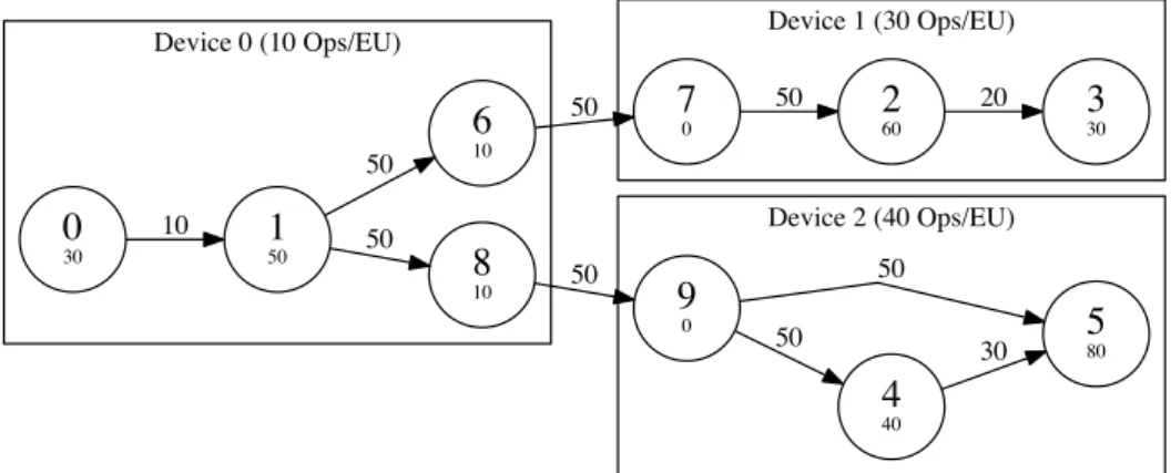
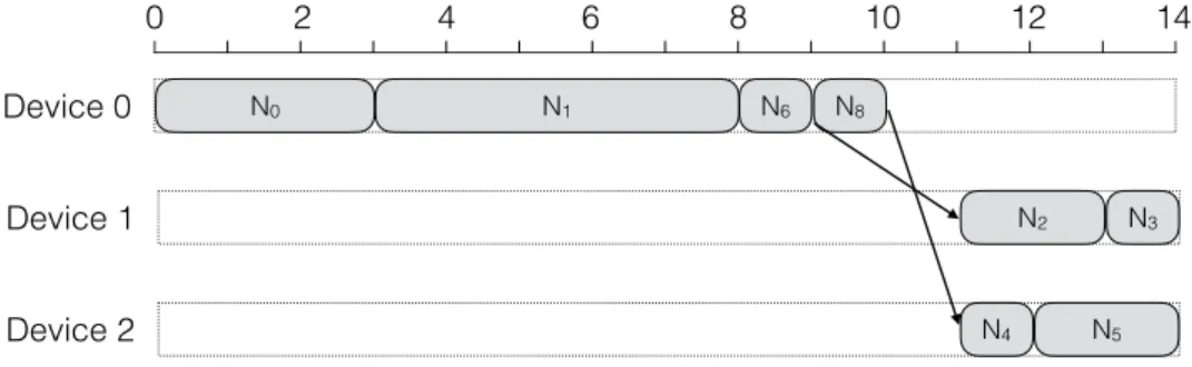
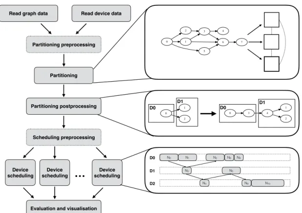
Figure 2.3 shows a partitioned graph. The nodes are labelled with their id and com-putation costs #ops. The tensor sizes are written on the corresponding edges. The abbreviation EU stands for execution unit. All abbreviations and function names are listed and explained in Table 2.2. The device speed of device 0 is 10 Ops_EU, the one of device 1 is 30 Ops_EU and device 2 is 40 Ops_EU fast. The transfer rate between device 0 and 1 is 25

EU while the transfer rate between device 0 and 2 is

50

EU.

At first, the execution times for each node are calculated by dividing the node’s number of operations with the device speed:

exec(n0) = #ops(n0) speed(d0) = 30Ops 10Ops EU = 3EU exec(n1) = #ops(n1) speed(d0) = 50Ops 10Ops EU = 5EU exec(n6) = #ops(n6) speed(d0) = 10Ops 10Ops EU = 1EU exec(n8) = #ops(n8) speed(d0) = 10Ops 10Ops EU = 1EU exec(n2) = #ops(n2) speed(d1) = 60Ops 30Ops EU = 2EU exec(n3) = #ops(n3) speed(d1) = 30Ops 30Ops EU = 1EU

(20)

Device 1 (30 Ops/EU) Device 0 (10 Ops/EU) Device 2 (40 Ops/EU) 0 30 150 10 6 10 50 8 10 50 7 0 50 9 0 50 2 60 50 4 40 50 5₈₀ 50 3 30 20 30

Figure 2.3: The graph is divided onto three machines. Each node has a node id (upper value) and number of operations (lower value). The labels on the edges represent the tensor size.

Table 2.1:Scheduling order per device Device Order (in node ids) 0 0, 1, 6, 8 1 7, 2, 3 2 9, 4, 5 exec(n4) = #ops(n4) speed(d2) = 40Ops 40Ops EU = 1EU exec(n5) = #ops(n5) speed(d2) = 80Ops 40Ops EU = 2EU

The receive nodes take zero execution units to receive the data. Moreover, the required time to transfer the computed results has to be taken into account:

transfer time(n6, n7) = weight(n6, n7) transfer rate(d0, d1) = 50 25 EU = 2EU transfer time(n8, n9) = weight(n8, n9) transfer rate(d0, d2) = 50 50 EU = 1EU

The scheduling algorithm defines the execution order as shown in Table 2.1. The resulting execution sequence is visualized in Figure 2.4. The computed data from node

(21)

2.6 Simplifications

6 arrives at device 1 after 11 execution units. To finish processing device 1 needs additional 3 units. At device 2 the data arrives after 11 execution units and it needs 3 units to finish processing. So the overall execution time is 14 execution units.

Device 0 Device 1 Device 2 N0 0 2 4 6 8 10 12 N1 N6 N8 N2 N4 14 N5 N3

Figure 2.4:Schedule of the sample graph shown in Figure 2.3

2.6 Simplifications

In order to reduce the model and problem complexity some less important parts are not taken into account.

With respect to TensorFlow multiple properties could be additionally considered: • Backpropagation: In order to adapt the model parameters, backpropagation is used

and information flows in the reverse direction of the dataflow graph [CZG+16] [Sca16]. Backpropagation is very specific to machine learning and could be modeled by inserting additional nodes and edges to the graph [MAP+15].

• Control flow nodes [MAP+15]: TensorFlow allows the usage of control flow nodes. With control flow operators, it becomes for example possible to express iterations, if-conditions or while-loops on dataflow graphs.

• Common subexpression elimination [MAP+15]: Redundant parts of the model are eliminated and computed only once. This approach helps to avoid unnecessary computation. If this procedure eliminates nodes and edges before partitioning, our model can also take this into account.

• Model replication [MAP+15]: In order to allow data parallel training the model is replicated. We can also express model replication by replicating the whole graph. If only parts of the graphs are replicated some edges have to be inserted to connect the "source" nodes of the replicated parts with its predecessors.

(22)

Table 2.2: Notation overview

G = (V, E, C) Graph with vertex set V, edge set E and colocations C

E ⊂(V ×V ×_N) Edge set consisting of tuples (start node, end node, weight)

D Device set

exec(nx) Execution units (time) necessary to compute nodenx #ops(nx) Number of operations necessary to compute node nx speed(dx) Speed of devicedx (in operations per execution unit) transfer time(nx,ny) Transfer time to transfer tensor from nx tony

weight(nx,ny) Weight of edge (nx,ny) (= tensor size) transfer rate(dx,dy) Transfer rate between device dx anddy

d(nx) Device on whichnx is placed by the partitioning algorithm. Is equal to -1 if the node is not placed yet.

type(dx) Type of devicedx, e.g CPU or GPU device constraint(n) Device constraint of node n

memory size(d) Memory size of device d

Vdx Set of all nodes assigned to devicedx

Vgx Set of all nodes being member of the colocation group gx

exec(d) Total execution time of device d

execmin(d) Minimal execution time possible if the device d would exe-cute all nodes sequentially without any idle times

#ops(dx) Sum of all nodes’ operations assigned to dx

EU Execution unit

Ops Operations

size(e) Size of the edge e = (ny, nx).

Equal to the output tensor size of nodeny

sizeest(n) Estimated size of a node n’s memory requirement. Sum of memory demand, output tensor size and input tensor sizes. pred(nx) Set of direct predecessor nodes of node nx

succ(nx) Set of direct successor nodes of nodenx

makespan Time period from computation beginning until the last device has finished execution.

assignment unit Colocation group or not colocated node (assigned as one unit during partitioning).

(23)

2.6 Simplifications

• Computation pipelining [MAP+15]. Smart pipelining would increase the benefits of partitioning in most cases and has no impact in the worst case.

• Subgraph execution [ABC+16]: Only parts of the model are executed. In our model, we assume that all nodes are executed exactly once. However, subgraph execution can be handled by treating the subgraph as a graph. Nevertheless, this is only efficient if the executed subgraph does not change very often. If this is the case, more dynamic partitioning approaches would be required.

The tensors sizes also depend on the input data [Sca16]. We assume that the tensor sizes stay the same and to know them in advance. The TensorFlow developers also state that their placement strategy does estimate fixed tensor sizes based on a cost model or simulated execution [MAP+15].

Another simplification is that a node’s execution duration is computed by its number of operations divided by the device speed. However, it could be different for each node device pair.

(24)

(25)

3 Approach Overview

This chapter provides an approach overview to solve the problem presented in Chapter 2. The first idea was to implement novel partitioning and scheduling algorithms within the TensorFlow library and compare them with already existing TensorFlow partitioning and scheduling algorithms. However, only a very simple placement algorithm is published by Google for now. Every node is mapped per default on the same device unless the user places the nodes manually. Additional factors like the cost model or memory constraints are not considered in the code published by Google, although described in the TensorFlow whitepaper [MAP+15]. The described scheduling strategy is also not available. This is the reason why we decided to develop an evaluation framework in Java.

3.1 Evaluation Framework

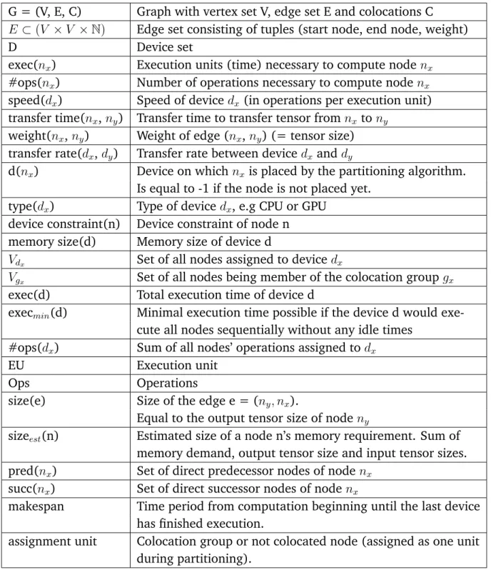
In order to be able to compare and implement partitioning and scheduling strategies faster and consider all the required constraints an evaluation framework has been devel-oped. In the following sections the components of this evaluation pipeline are described. Figure 3.1 shows these components. At first, device and graph data is read and coloca-tion groups are calculated. Some particoloca-tioning algorithms require certain preprocessing steps which are executed during the partitioning preprocessing. Afterwards, the graph is partitioned onto multiple devices and send and receive nodes are inserted during partitioning postprocessing. Depending on the scheduling strategy, some preprocessing steps are necessary. Subsequently, the scheduling is performed on each device. At the end of the computation, the results are collected and visualized.

Every part of the framework can be implemented independently. Furthermore, partition-ing and schedulpartition-ing algorithms can be integrated and exchanged easily.

(26)

Read graph data Partitioning preprocessing Partitioning Device scheduling Device scheduling Device scheduling

Evaluation and visualisation

D0 D1 D2 N1 N2 N6 N8 N9 N5 N0 N3 N4 N10 0 1 2 0 3 4 1 2 D0 D0 D1 D1 0 1 2 5 3 6 4 7 Read device data

Partitioning postprocessing

Scheduling preprocessing

…

Figure 3.1:Evaluation framework pipeline and its components

3.1.1 Device and Graph Reader

In order to evaluate the strategies, dataflow graphs are extracted from TensorFlow. On top of that, sample synthetic graph and device data is created in order to test various graph and device combinations. The properties of these graphs and devices are further described in Chapter 6.

Within the evaluation framework a device reader is responsible for reading the device data from a csv-file. A custom graph reader reads the graph information from a specified file. It does not matter if the graph data is synthetic or extracted from TensorFlow: It is stored in an equal structure as csv-file.

(27)

3.1 Evaluation Framework

Algorithmus 3.1Calculate colocation groups static int componentId = 0;

procedure READ_NODE(nx)

ColocationComponent component;

for alln ∈col(nx)do

//colocationId -1 means that the node is not in any colocation group yet

ifn.colocationId == -1then ifcomponent == nullthen

//when creating a new component it is stored in a set of components component = new Component(componentId);

componentId ++;

end if

//in addNode the colocationId of n is also set component.addNode(n);

else

ifcomponent == nullthen

component = ColocationComponent.getComponentForId(n.colocationId); else //union component.merge(ColocationComponent.getComponentForId(n.colocationId)); end if end if end for end procedure

3.1.2 Partitioning Preprocessing

When reading the graph data, colocation groups are calculated. Algorithm 3.1 shows the algorithm which generates the colocation groups. Whenever a node nx is colocated all its colocated nodes col(nx)are checked. If the nodeny ∈col(nx)is not in a colocation group yet it is added to the colocation group of nx. If it is already in a colocation group the two colocations groups are merged. If two colocation groups are merged or a node is added to a colocation group the device constraint has to be checked. If member nodes have contradictory device constraints the input data is invalid and an exception is thrown. For a short and clear notation, we assume that nx is also a member of col(nx) in Algorithm 3.1.

Depending on the partitioning strategy other preprocessing steps are taken. If this is necessary for a partitioning strategy it is described more detailed in the partitioning chapter 4.

(28)

3.1.3 Partitioning

A partitioning algorithm splits the nodes on different devices and determines which node is placed on which device. Some devices might not be feasible for a specific node. To decide if a node can be placed onto a specific machine the following factors have to be considered:

• Colocation constraints

• Device constraints: Can the node be executed on a specific device type? • How much memory is left on a device

3.1.4 Partitioning Postprocessing

The required send and receive nodes have to be inserted for cross-device edges. When a node is assigned during partitioning all direct predecessor and successor nodes are checked if they are placed on a different device. If so, the node is added in a set of nodes with cross-device edges. After partitioning new nodes are inserted by making use of these sets. If a node has outgoing cross-devices edges to the same device only one send-receive-node-pair is inserted as described in Figure 2.2 in Section 2.4.

3.1.5 Scheduling Preprocessing

Depending on the scheduling algorithm various preprocessing computations are neces-sary. If this is the case, they are described in the scheduling chapter 5.

3.1.6 Scheduling

The scheduling algorithm determines which node is executed next. In the system model only non-preemptive scheduling is supported which means that a node is executed completely once started. The scheduling algorithm has to consider the data dependencies in the dataflow graph. A node can only be executed when all its direct predecessor nodes have finished computation.

A node’s calculated data is kept in RAM as long as its direct successor nodes have not started computation. Therefore, a mechanism similar to reference counting has been implemented to find out when the data is no longer needed and can be deleted. A counter is initialized on the number of direct successors. This counter is decremented

(29)

3.2 Timing Behaviour

each time a direct successor node executes. If the counter reaches zero the result can be deleted.

3.1.7 Evaluation

Multiple metrics are possible to evaluate the scheduling and partitioning strategies. The first goal is to fulfil all the required constraints like device, colocation and memory constraints as a violation leads to an invalid partitioning. To measure the quality of the partitioning and scheduling algorithms, two metrics are taken into account: The network traffic and execution time which were defined in Section 2.3 The results of a computation are stored in csv-files and automatically visualized by matplotlib in python scripts.

3.2 Timing Behaviour

When simulating the scheduling, synchronization and communication between the devices’ local time has to be considered to ensure the correct simulation of an execution pass. One approach might be to use the real world time as time synchronization mechanism. Consequently, the whole simulation would have to be implemented in a distributed system with all the programming overhead e.g. for message exchange. It would also be difficult to run the graphs exactly with the specified values like the transfer rate or to change certain values to evaluate different situations. Using real world time as synchronization mechanism leads to another disadvantage: One has to run the node computation in real time which could lead to a long evaluation duration.

For these reasons, a simulated timing behaviour is preferable. However, if each device has its own local timestamp it is necessary to avoid messages arriving in the future which would have had an influence on past decisions.

To illustrate this problem an example graph is provided in Figure 3.2. The node’s upper value is the id and the lower value represents the node’s #ops. The edges are labelled with their tensor sizes. In this example a parallel simulation is assumed without any synchronization mechanisms. The transfer rates and device speeds are 1

EU. The simulation starts with device 2 and computes 50 EU as execution duration for node 7. The data arrive time of node 7’s output tensor is computed to be at 80 EU. Device 1 becomes active in the simulation, executes node 5 and sets its local timestamp to 110 EU.

(30)

Device 0 Device 2 Device 1 1 30 210 10 3 10 10 4 20 50 5 30 7 50 30

Figure 3.2:Sample graph labelled with node id, #ops and edge weigths

However, device 0 has simulated the execution of node 1 and 2 with an execution duration of 40 EU. The data is calculated to arrive at device 1 after 50 EU. The problem is that the local timestamp of device 1 is already at 110 EU in the simulation. Nevertheless, device 1 would have been able to execute node 3 after 50 EU if the simulation would have been implemented correctly. This is the reason why it is very important to have received all past data before making any scheduling decisions in the simulation.

To avoid making decisions without knowing all executable nodes at a specific timestamp the local timestamp of each device is collected. The device with the lowest local timestamp is selected to make the next scheduling decision. This algorithm has the disadvantage that the simulated scheduling can not be ran in parallel but also avoids the problem of making wrong scheduling choices or idle unnecessarily.

(31)

4 Partitioning

In this chapter various partitioning algorithms are described as well as their corre-sponding preprocessing steps. At first, the partitioning problem is defined formally. Afterwards, multiple partitioning strategies and their corresponding preprocessing steps are described.

A graph G = (V, E, C) consists of a set of vertices V = {v0, v1, ..., vr} and directed weighted edges E ⊂ (V ×V ×_N). As described in Section 2.2 a vertex is defined by an id, operation costs and a device constraint. The in C ⊂ (V ×V)contained tuples

(vx, vy)∈C define vertices which have to be assigned to the same device.

The goal is to divide the graph’s nodes onto n devices D = {d1,d2, ..., dn} into disjoint subsets. Devices are defined by an id, device type (CPU, GPU, TPU), memory size and speed. Abbreviations and functions are listed in Table 2.2. An assignment a: V→D has to be created by the partitioning algorithm meeting the following constraints:

1. ∀(vx, vy)∈C :d(vx) = d(vy)

2. ∀v ∈V :type(d(v)) =device constraint(v)∨device constraint(v) =ALL

3. ∀d∈D: P v∈V_dx

sizeest(v)< memory size(d)

and minimizes together with the scheduling algorithm the following parameters: 1. execution time (previously defined in Equation 2.1)

2. network traffic (previously defined in Equation 2.2)

In the following, we call a colocation group or a not colocated node an assignment unit. Colocated nodes have to be mapped to the same device which is why we will assign them in one pass. Colocation groups and a not colocated nodes share the properties of a device constraint and memory demand.

(32)

1. The assignment unit’s device constraint is equal to the device type or no device constraint exists.

2. The device has enough memory to be able to assign the whole assignment unit.

4.2 Hashing

Hashing is a very simple, well-known and fast placement strategy. Because of the colocation groups, memory and device constraints it is slightly modified to the following algorithm:

Iterate over colocation groups and try to assign them. For each colocation group a hash value is calculated based on the number of already assigned colocation groups modulo the number of devices. The device whose id is equal to the hash value is checked to be feasible or not. If a device is not feasible, search iteratively for the next feasible device and assign every node of the colocation group. After all colocation groups are assigned iterate over not colocated nodes and assign them to a feasible device in the same manner as the colocation groups.

4.3 HEFT

The Heterogeneous Earliest Finish Time (HEFT) [THW02] algorithm maps nodes to devices iteratively. It consists of two phases: The task prioritizing phase and the processor selection phase.

In the task prioritizing phase, the nodes are ranked due to their upward rank which describes the computation costs and data transfer costs from the given node to the "last" sink node. As soon as the upward ranks are computed the tasks are sorted in a descending order. In this order the tasks are assigned to processors within the processor selection phase.

In the processor selection phase the earliest finish time of a node for each device is computed in an insertion based manner. The maximum of the predecessor nodes’ finish time and the required transfer time is taken as the earliest point of time in which the task can possibly start executing. Starting at this computed time each device is checked in order to find a time slot which is big enough to insert the task into. The node is assigned to the device with the lowest earliest finish time.

In order to meet the special constraints (e.g. colocation or device constraints) the HEFT algorithm was slightly modified. The earliest finish time is only computed on the

(33)

4.4 Batch Split

feasibledevices, as a node can not be assigned to the other devices anyway. If the node is colocated, all colocated nodes have to be assigned to the same device. However, their predecessor nodes might not be assigned yet which is why the earliest finish time can not be computed for these nodes. So their computing time slot is only defined and added to the devices’ time schedule when it is their turn due to the task prioritizing list.

4.3.1 Upward Rank

The upward ranks are an essential element in the task priorization phase. In the evaluation framework they are calculated in the partitioning preprocessing phase. The upward rank of a node ni is defined as the average computation costs ω¯i plus the maximum of the successors’ upward ranks and average communication costsc¯i,j of the edge from ni tonj (see [THW02]):

ranku(ni) = ¯ωi+ max nj∈succ(ni)

( ¯ci,j+ranku(nj)) (4.1) The upward rank of a sink nodensis equal toω¯s. In the paper the average execution cost

¯

ωi for task i is calculated in a slightly different way, as they have estimated execution times for each task-processor pair. We define the average computation costsω¯i as #_speedops(_avrni), whilespeedavr is defined as the following:

speedavr = P d∈D

speed(d)

|D| (4.2)

The calculation of the average communication cost is quite similar. The transferred data between two nodes is divided by the average transfer rate. The startup communication cost is considered in the computation costs of a send node. However, it is not processor specific at the moment. These average values are used as the placement decisions are not made yet.

4.4 Batch Split

In the Batch Split partitioning the graph’s set of nodes is divided into different ranges. For each node the operations source rank as well as the operations sink rank is computed. The operations rank is used to sort the nodes in a descending order. The nodes of the critical path which should not be delayed are very likely to be all in the highest range. The nodes are assigned to the devices (also sorted based on their speed) with an assignment of the nodes of the highest range to the fastest device. Clearly, this is not

(34)

possible if a device is not feasible. Therefore, each node is assigned to the next feasible device which can be found in a similar way like in hashing. If a colocated node is in a range and is not already assigned yet, the whole colocation group is assigned as one unit.

The complexity of this algorithm isO(n×log(n))as the whole node set has to be sorted. The assignment of the nodes and calculation of the operations rank is possible in linear time.

4.4.1 Operations Rank

The operations rank is defined as sum of operations sink rank and operations source rank and is used to rate the “importance“ of a node.

Operations source rank counts the number of operations required to reach the given node from a source node and be able to execute it. This is expressed in Equation 4.3.

operations source rank(ni) = max nj∈pred(ni)

(operations source rank(nj) + #ops(nj)) (4.3) Operations sink rank counts the number of operations required to execute the current node and the longest path to a sink node which is formulated in Equation 4.4.

operations sink rank(ni) = ( max nj∈succ(ni)

operations sink rank(nj)) + #ops(ni) (4.4)

4.5 Iterated Critical Path

The basic idea for the Iterated Critical Path (ICP) strategy is to assign paths iteratively to devices as one unit. Thereby, we want to keep especially the first extracted critical path on the same device. This is only possible as long as there are no contradicting memory, device or colocation constraints. If so, the path has to be split.

This strategy is more computationally expensive than the other ones. The current critical path can be found in linear time but this procedure has to be repeated till no edge is left.

1. Get the critical path:

a) Start at the source nodes and compute for each node the operations source rank. Extend the algorithm to set a path predecessor node for each node which is the one the maximum operations source node value is taken from.

(35)

4.6 Critical Path

b) Iterate over the sink nodes and take the one with the maximum operations source rank. This sink node is on the critical path.

c) Create a new path. Add the sink node to this path and follow the path predecessor nodes adding them to the path as well. Continue till there is no path predecessor node left which means that the whole path is traversed. Generate subpaths while adding nodes to the path based on already assigned nodes or contradicting device constraints. If a node is already assigned, it is not added to any subpath and finishes the current created subpath.

d) Remove the path’s edges. Add the newly created sink or source nodes to the sink or source node sets.

2. For each subpath, check feasible devices and choose the device which has the minimum possible execution time execmin so far. As shown in Equation 4.5 execmin(d) is equal to the number of operations assigned to device d divided by the device speed. Consequently, it stands for the minimal execution time possible if all nodes are executed sequentially without any idle times.

execmin(d) =

#ops(d)

speed(d) (4.5)

If there is no feasible device further split the subpath in order to reduce the memory demand.

3. Continue until all nodes are assigned.

4.6 Critical Path

The Iterated Critical Path strategy is quite computationally intensive. It might not be necessary, to split the graph into paths until no path is left. For the above reason, the partitioning strategy Critical Path (CP) is introduced:

Compute the critical path based on upward ranks in the same manner as at the Iterated Critical Path partitioning. Assign the nodes of this path (as well as the nodes which are colocated with these nodes) on the fastest feasible device. Take the other nodes and assign them iteratively to the feasible device with the minimum possible execution time execmin.

In comparison to the Iterated Critical Path, this strategy is much faster. Depending on the graph, many evaluations showed that there is a long critical path and all the other

(36)

extracted paths are pretty short. In these cases, it could be worth to save partitioning ex-ecution time, only assign the first extracted critical path and switch to a computationally less intensive method afterwards.

4.7 MITE

The idea of the partitioning strategy MITE is to consider multiple factors and use a heuristic function to assign the nodes. MITE stands for the different factors Memory,

Importance speed boost, Traffic and Execution time. These factors aim to minimize the transferred data and the overall execution time. Moreover, devices which have proportionately much free memory in comparison to their total memory are preferred. Important nodes (based on their effect on the overall execution time) should be located on faster devices.

At first, the colocation groups are assigned and after that the not colocated nodes are placed. All feasible devices are checked and the assignment unit a (colocation group or not colocated node) is assigned to the device which minimizes the following function shown in Equation 4.6

heu(dx, a) =traffic(dx, a)×

execution time(dx, a)× memory(dx)×

importance speed boost(dx, a)

(4.6)

The traffic component is supposed to minimize the transferred data size, whereas the factor execution time should lead to a low overall execution time. The factor memory is supposed to favor devices with not much memory used, while importance speed boost influences important nodes to be mapped on faster devices. These factors are now explained more detailed.

As shown in Equation 4.7, traffictemp depends on the node to be assigned and the device

dx to be checked as potential assignment device. The edge weight is divided by the transfer rate as a transfer of large data sizes is far worse for the execution time on a slow connection than on a high speed connection.

The transferred tensor size of all direct predecessor and successor nodes is considered, as long as they are already assigned and not located on the same device. One might also consider nodes which are not assigned yet. At the moment a not assigned node leads to zero increase in the traffic but is definitely worse than a node located on the

(37)

4.7 MITE

same device which also results in a zero increase. There are different possibilities how a not assigned node can be handled. At the moment the best case placement (the one on the same device) is assumed. Another option would be the worst case placement which would be on the device with the slowest connection on which no send-receive-node-pair for this data transfer exists yet. Moreover, one could take simply the average.

traffictemp(dx, ni) = X nj∈pred(ni) d(nj)̸=dx d(nj)̸=−1 ( weight(nj, ni) transf er rate(d(nj), dx) ×condpred(nj, dx)) + X nj∈succ(ni) d(nj)̸=dx d(nj)̸=−1 ( weight(ni, nj) transf er rate(dx, d(nj)) ×condsucc(ni, d(nj))) (4.7)

However, the aggregation of send and receive nodes has to be considered for the traffic which is the reason forcondpred(nj, dx)andcondsucc(ni, dj).

The idea ofcondpred(nj, dx) (as shown Equation 4.8) is that only the weights of edges with predecessor nodes matter which have not already another successor node on the devicedx. If there is another successor ondx, there was already a send-receive-node-pair inserted and no additional data would have to be transferred.

condpred(nj, dx) =         

0 , if predecessor nodenj has already another successor node on devicedx

1 , otherwise

(4.8)

condsucc(ni, dj) (as shown Equation 4.9) checks if there is already another successor node of ni on device dj. If so, no additional send-receive-node-pair is needed.

condsucc(ni, dj) =  



0 , if another successor node ofni is on devicedj

1 , otherwise (4.9)

If a is a colocation group the sum of the member nodes’ traffic has to be taken as expressed in Equation 4.10.

(38)

traffictemp(dx, a) =     

traffictemp(dx, ni) , if a is the not colocated nodeni P

ni∈Vg

traffictemp(dx, ni) , if a is the colocation groupg

(4.10)

However, traffictemp(dx, a)can not be used directly as it has to be normalized. This is achieved by dividing by the maximum traffictempof all feasible devices. Obviously, this can only be done if the maximum traffic is not zero. If traffictemp is zero, the traffic (as shown in Equation 4.11) is set to a very small number in order to avoid that all other factors in Equation 4.6 are not considered anymore. We define_tˆ_{as the maximum}

traffictemp value of all feasible devices.

traffic(dx, a) =          0.000001 , if traffictemp(dx, a)= 0∧ˆt̸=0 1.0 , iftˆ= 0 traffictemp(dx,a) ˆ t , otherwise (4.11)

The factor execution time shall minimize the overall execution time. Therefore, the number of already assigned operations is taken in addition to the number of operations of the checked assignment unit. The sum is divided by the device speed and the result is the minimal execution time of this device if the assignment unit would be on this device. This is expressed in execution timetemp as shown in Equation 4.12. The idea is that the overall execution time is minimized if the maximum execution time of all devices is minimized.

execution timetemp(dx, a) =      #ops(dx)+P ni∈Vg#ops(ni)

speed(dx) , if a is the colocation group g

#ops(dx) + #ops(ni)

speed(dx) , if a is a not colocated nodeni

(4.12) For normalization, the execution timetemp has to be divided by the maximum execution timetemp eˆof all devices. If this ˆeis zero, the execution time is set to 1.0 as shown in Equation 4.13. execution time(dx, a) =    1.0 , ifeˆ= 0

execution timetemp(dx,a)

ˆ

e , otherwise

(4.13)

As devices with not much memory used should be favored, the factor memory(dx)simply calculates the portion of used memory for device dx. If there is no memory used on

(39)

4.8 Depth First Search

devicedx yet, memory(dx)is set to one tenth of the minimal non zero memory portion ˜

m of all devices as expressed in Equation 4.14. m˜ is initialized to 1.

memory(dx) =    ˜ m 10.0 ,memory portion ofdx= 0 used memory ofdx

memory size(dx) ,otherwise

(4.14)

The factor importance speed boost shall lead to the assignment of important nodes on fast devices. The more important the node or the colocation group is the closer is importance(a) (shown in Equation 4.16) to 1. The faster a device is the closer is speed(dx) divided by the speed fˆof the fastest feasible device to the maximum of 1. As the device which minimizes the Function 4.6 is used for the assignment, the product has to be subtracted by 1 as shown in Equation 4.15. In general, faster devices should be favored by this factor which is why we did not simply take the absolute value of the difference between the importance and speed factor.

importance speed boost(dx, c) = 1−(importance(c)∗

speed(dx) ˆ

f ) (4.15)

The importance differs if a is a colocation group or a not colocated node and is defined in Equation 4.16. The importance of a node is given by its operations rank and divided by the maximum operations rankoˆwhich is given by nodes on the critical path.

importance(a) =              P ni∈Vg operations rank(ni) ˆ

o×|Vg| , if a is the colocation groupg

operations rank(ni)

ˆ

o , if a is a not colocated nodeni

(4.16)

4.8 Depth First Search

Another partitioning strategy is Depth First Search (DFS) partitioning. The idea behind this strategy is to traverse the graph in a depth first search and assign the nodes based on a heuristic function.

The algorithm performs the following steps:

Sort the source nodes in a decreasing order based on their operations rank. Traverse the graph in depth first search starting at the beginning of the sorted list. Consequently, the algorithm starts with a source node which is on the critical path.

(40)

Perform the depth first search with the help of an already-visited-boolean and a recursive function. If a node is not assigned yet, assign the whole assignment unit. Place the assignment unit on the device minimizing the product of execution time and traffic which was defined in the MITE strategy.

(41)

5 Scheduling

As illustrated in Chapter 1, scheduling plays an important role in minimizing the overall execution time. In this chapter we define the scheduling problem and present three scheduling algorithms.

A scheduling algorithm defines the execution order for each device. The function

ex_order:Vd →S maps all the device’s vertices on natural numbers which define the order of execution. The set S does not contain duplicates and is defined as S ={n ∈

N|n ∈S∧y∈S→n ̸=y}.

For a correct scheduling the following criteria have to be fulfilled: 1. A node is executed only once.

2. Each node is executed.

3. Each device can execute at most one node simultaneously.

4. Once a device has started to execute a node, it can not be interrupted. (→non-preemptive scheduling)

5. A node n can be only executed as soon as all tensors of its direct predecessor nodes are computed and transferred to the device d(n). When all data is available, the node is called an executable node.

6. A device can only execute nodes which are placed on this device. A node can not be on multiple devices.

7. A device can only compute nodes if there is an executable node on this device. Idling is possible.

(42)

The overall goal is to minimize the makespan as defined in Equation 2.1. The graph is already partitioned when the scheduling starts. As the scheduling algorithm has no influence on the number of cross-device edges and every node is executed exactly once, the traffic parameter is independent from the chosen scheduling strategy.

5.2 FIFO Scheduler

For each device, the nodes which can be executed are stored in a collection. Whenever, a new node becomes executable it is added to the collection and is removed as soon as it was executed. At First In First Out (FIFO) scheduling the collection is a queue. Devices execute the nodes in the same order the nodes have been added to the queue.

5.3 PCT Scheduler

The upwards Path Computation Time first (PCT) scheduler executes the node first whose longest path of direct and indirect successors takes most time to compute. This can be achieved by selecting the executable node with the maximum upwards path computation time. The (upwards) path computation time (PCT) is calculated starting from the sink nodes as shown in Equation 5.1. The path computation time value of a sink node

ni is the time it takes to execute ni on the device it was assigned to. If the node is not a sink node one has to consider the maximum of the time to transfer the data to one of its successor nodes as well as the path computation time of the same successor node additionally. The transfer time is 0, if both nodes are placed on the same device. Otherwise, it is the edge weight divided by the transfer rate between the two devices.

PCT(ni) = max nj∈succ(ni) (PCT(nj) +transfer time(nj, ni))+ #ops(ni) speed(d(ni)) (5.1) The path computation time is calculated once in linear time during the scheduling preprocessing.

5.4 MSR Scheduler

The PCT scheduler only considers the path computation time for its scheduling decisions. However, if a lot of nodes depend on a specific node it could be better to schedule this

(43)

5.4 MSR Scheduler

D0

D1

0 50 5 50 10 1 50 10 6 50 10 7 50 10 8 50 10 2 50 10 3 50 10 4 350 10

(a)Graph containing the #ops per node

D0

D1

0 11 5 5 1 10 6 3 72 18 2 9 38 74

(b)Graph containing the path computation time per node

D0 D1 N0 D0 D1 N1 N2 N3 N4 N5 N6 N7 N8 N0 N5 N1 N2 N3 N4 N6 N7 N8

(c)Schedule of scheduling option 1 D0 D1 N0 D0 D1 N1 N2 N3 N4 N5 N6 N7 N8 N0 N5 N1 N2 N3 N4 N6 N7 N8

(d)Schedule of scheduling option 2

Figure 5.1: Scheduling strategies

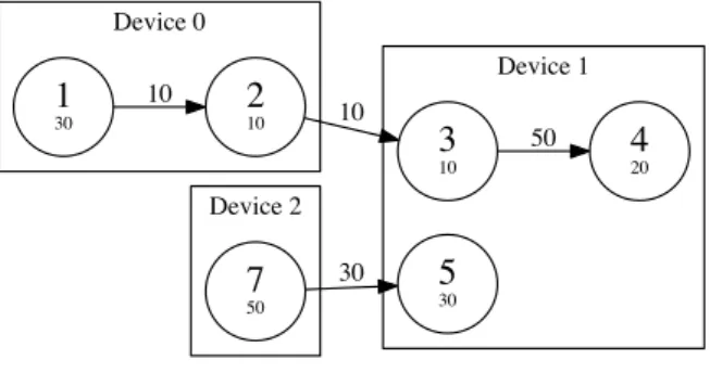
node first even if another one has a larger path computation time. This is especially the case if another idle device becomes active as a successor node becomes executable. Schedules created by two different scheduling strategies on the same graph are illustrated in Figure 5.1. The assumed device speed is 50 Ops_EU, while the transfer rate is 10

EU. Figure 5.1 (a) shows the dataflow graph annotated with node and edge weights. In Figure 5.1 (b) the nodes are labelled with their path computation time values. The schedule created by the PCT scheduler is visualized in 5.1 (c). Clearly, the schedule in Figure 5.1 (d) would be better as the overall execution time is much smaller.

Therefore, the new scheduling strategy Maximum Successor Rank first (MSR) is intro-duced in which nodes are selected based on the function successor rank in Equation 5.2. Each direct successor node of ni increases the successor rank by one. ni gets an additional point for each successor node which is not assigned to the same machine and another one for each successor becoming executable after computing ni. This is formulated by prednotex(n) which contains the not executed predecessor nodes of n. After executing the last not executed predecessor node, the node becomes executable. The last term is an increase of 5 for each successor which becomes executable on an idle device. This is rewarded by so many points as a device becomes active again and

(44)

thereby probably reduces the overall execution time. The function idle(d) is 1 if device d is idle when making the scheduling decision. If not, it is 0.

successor rank(ni)= X nj∈succ(ni) ( 1 + 1∗(d(nj) ! = d(ni)) + 1∗(|prednotex(nj)|== 1)

+ (idle(d(nj))∧(|prednotex(nj)|== 1))∗5 )

(5.2)

The idea is to favor the execution of nodes whose successor nodes can be executed afterwards and especially if it leads to a device becoming active. If all the rank values are equal, the path computation time is used as a tie breaker.

An obvious disadvantage of this strategy is that we have to check if another device is idle or not. This requires additional device communication while scheduling.

(45)

6 Sample Data

In order to evaluate partitioning and scheduling strategies sample data has to be collected. In this chapter typical model types of TensorFlow are described. Furthermore, extracted graph and cost models are analysed in order to generate realistic synthetic data.

Two kinds of graphs are used for the evaluation:

1. Real-world dataflow graphs extracted from TensorFlow and extended by required constraints.

2. Synthetic dataflow graphs

6.1 Typical Examples in TensorFlow

Typical machine learning models can be expressed in TensorFlow. In order to get a TensorFlow dataflow graph, a model has to be defined and exported [Sca16]. A typical model type is a linear model which is a weighted sum of variables assuming a linear relation between its input variables and output variable. It can be used to predict continuous values or to classify. In comparison to multi-layer networks, it can be quicker debugged and trained and works well with many features.

Another typical model type are convolutional neural networks. Convolutional neural networks suit well for data which can be structured as a grid in a way that related values are next to each other. Therefore, they are often used for image classification [CZG+16] [KSH12] and contain convolutions as the name suggests. Convolution is a mathematical operation that takes two functions as an input and provides another function as output. Practically, one can think of a convolution for example as sliding a kernel over the pixels of an image.

Recurrent neural networks are another typical model type and are for example used for language modeling [MAP+15] [CW08]. They often consist of multiple layers with recurrent connections.

(46)

6.2 Data Generation and Sample Data

To evaluate partitioning and scheduling algorithms, sample data has to be collected. Therefore, different models in TensorFlow are generated and the graph as well as the cost model is extracted. Different configuration options have to be set that the cost model can be extracted. Information about the graph can be received by calling “tf.get_default_graph().as_graph_def()“ in python.

The extracted graph data contains the name and id of existing nodes, how these nodes are connected (“input: “Variable_1“ “) and which nodes are colocated (“loc:@Variable_1“). The cost model contains information about the compute costs. TensorFlow also collects information about the nodes’ memory sizes or edges’ tensor sizes but they are not easily extractable yet. For the evaluations the data is extended by the tensor sizes, #ops, device constraints and RAM demand.

As the TensorFlow sample models are not that large yet (~5000 nodes) other data sources were required. A random graph generator was implemented in order to create directed acylic graphs provided with the required characteristics. These characteristics include the id, incoming and outgoing edges, colocated nodes, the tensor size of the output tensor, #ops, RAM demand and the device constraint for each node. A graph is generated in levels. As an edge is always from a node of a lower level to a node of a higher level cycles are avoided. Multiple ways to generate the edges were implemented: When a new level was generated each node of the former levels is linked with a defined probability to each node in the new level. The drawback of this approach is the following: With each new level all existing nodes are linked to the latest inserted nodes with a defined probability. Hence, the lower the level the higher the probability for a node to have many edges. To get a more realistic distribution of edges, a limitation on the levels can be added e.g no edge can be between nodes with a distance higher than 5 levels. Alternatively, a function can be used to lower the probability of having an edge drastically the more distant two nodes are in terms of levels. In order to allow long range edges a method was implemented which randomly selects two nodes and adds an edge from the node with the lower level to the node with the bigger one. The edge is only added if the edge has not existed yet.

These typical graph characteristics depend on multiple input parameters: The number of levels as well as the minimum and maximum number of nodes per level. Furthermore, the minimum and maximum RAM demand to store a node can be defined. In order to set the size of a node’s output tensor the minimum and maximum tensor size can be provided. The number of operations for a node are set to be in a certain range as well. A node’s probability to have a GPU or CPU constraint is provided. Depending on how

(47)

6.2 Data Generation and Sample Data

(a)Convolutional network1 _(b)_{Recurrent network}2

(c)Dynamic recurrent neural network3

Figure 6.1:Size and number of colocation groups

the edges are generated the edge probability, an edge level limit or a function defining the edge probability can be set.

In order to add realistic colocation constraints we analysed the colocation groups in the graphs extracted from TensorFlow.

1_{https://github.com/aymericdamien/TensorFlow-Examples/blob/master/examples/3_} NeuralNetworks/convolutional_network.py (last followed on 28.02.2017)

2_{https://github.com/aymericdamien/TensorFlow-Examples/blob/master/examples/3_} NeuralNetworks/recurrent_network.py (last followed on 28.02.2017)

3_{https://github.com/aymericdamien/TensorFlow-Examples/blob/master/examples/3_} NeuralNetworks/dynamic_rnn.py (last followed on 28.02.2017)

(48)

Figure 6.1 shows the size and number of colocation groups in three different graphs extracted from TensorFlow. These graphs consist of many small colocation groups with just a few member nodes, while there are only few groups with many colocated nodes. For the evaluations, the edge weights are set randomly in a range of 1 and 100 as well as the number of operations per node. The memory demand of a node is also set randomly within this range.

The device data is also stored in a csv-file. Each device consists of a device id, available RAM, speed (number of operations per execution unit), the device type as wells as a transfer rate to all other devices. The transfer rate is encoded as an upper triangular matrix as the transfer rate of a device with an other device is bidirectional and a device has zero costs to communicate with itself.

When generating the device data, the number of devices can be set as wells as the device type probability. For the evaluations, the probability to be a CPU device is 60 % and being a GPU device is 40 %. The device speed is in a random range of 10 and 100 operations per execution unit. The faster a device is the less memory it has. The transfer rate between the devices is set to a random number in the range of 10 and 60.

(49)

7 Evaluation

In this chapter the partitioning strategies are evaluated in combination with the afore-mentioned scheduling algorithms. At first, the algorithms are executed on synthetic sample graphs and later on three graphs extracted from TensorFlow. Further evaluations are done on only seven devices. For these executions, we analysed the device utilization in order to investigate the reason for differences in the total execution time.

7.1 Synthetic Graph Evaluations

Various synthetic graphs were generated in order to evaluate combinations of scheduling and partitioning strategies. The properties of these graphs are listed in Table 7.1. The graph’s edges were generated on two different modes: The level based approach and a random method to allow long range edges. These techniques were further described in Chapter 6. The graphs vary for example on their number of nodes, density or portion of colocated nodes. The reason for these variations is that a strategy might perform well on certain graphs but worse on others.

Six different partitioning strategies were executed in combination with three different scheduling strategies on 100 devices. Some of the strategies are non-deterministic as e.g. the order of nodes being assigned might differ. In order to avoid false conclusions the visualized execution time is the average of 10 executions and the standard mean deviation is shown as a grey line on each bar.

Table 7.1: Properties of six synthetic graphs Graph #nodes #edges

(total) #random edges #level based edges #levels Minimum nodes per level Maximum nodes per level Edge level limit Average node degree #colocated nodes 1 36319 16076 8003 8073 300 50 200 20 0,44 5200 2 18168 25148 5015 20133 300 20 100 20 1,38 2762 3 7475 49510 0 49510 1000 5 10 3 6,62 263 4 9899 42486 21099 21387 200 20 80 10 4,28 1945 5 10440 47414 23535 23879 200 20 80 10 4,54 4768 6 26887 107144 53423 53721 500 10 100 20 3,98 4214

(50)

Figure 7.1 shows the simulated execution time of these scheduling and partitioning combinations. If the partitioning and graph combination stays the same, the FIFO scheduling strategy performs almost always the worst. In few cases the Maximum Successor Rank first (MSR) scheduling is slightly worse. The upwards Path Computation Time first (PCT) scheduling outperforms the other two scheduling strategies in almost all cases. Only in combination with MITE and Hashing, the MSR scheduler showed minimal better results in some runs on graph 1 and 2. We keep in mind that the path computation time value is used as a tiebreaker in the MSR strategy. However, this could be an explanation