Nottingham.
Access from the University of Nottingham repository: http://eprints.nottingham.ac.uk/29142/1/ktl-ethesis-corrected.pdf
Copyright and reuse:
The Nottingham ePrints service makes this work by researchers of the University of Nottingham available open access under the following conditions.
· Copyright and all moral rights to the version of the paper presented here belong to the individual author(s) and/or other copyright owners.
· To the extent reasonable and practicable the material made available in Nottingham ePrints has been checked for eligibility before being made available.
· Copies of full items can be used for personal research or study, educational, or not-for-profit purposes without prior permission or charge provided that the authors, title and full bibliographic details are credited, a hyperlink and/or URL is given for the original metadata page and the content is not changed in any way.
· Quotations or similar reproductions must be sufficiently acknowledged. Please see our full end user licence at:
http://eprints.nottingham.ac.uk/end_user_agreement.pdf A note on versions:
The version presented here may differ from the published version or from the version of record. If you wish to cite this item you are advised to consult the publisher’s version. Please see the repository url above for details on accessing the published version and note that access may require a subscription.
Portfolio Optimization
Khin Thein Lwin, BSc (Hons)
Department of Computer Science
University of Nottingham
A thesis submitted for the degree of
Doctor of Philosophy
Portfolio optimization involves the optimal assignment of limited cap-ital to different available financial assets to achieve a reasonable trade-off between profit and risk objectives. Markowitz’s mean variance (MV) model is widely regarded as the foundation of modern port-folio theory and provides a quantitative framework for portport-folio op-timization problems. In real market, investors commonly face real-world trading restrictions and it requires that the constructed port-folios have to meet trading constraints. When additional constraints are added to the basic MV model, the problem thus becomes more complex and the exact optimization approaches run into difficulties to deliver solutions within reasonable time for large problem size. By introducing the cardinality constraint alone already transformed the classic quadratic optimization model into a mixed-integer quadratic programming problem which is an NP-hard problem. Evolutionary al-gorithms, a class of metaheuristics, are one of the known alternatives for optimization problems that are too complex to be solved using deterministic techniques.
This thesis focuses on single-period portfolio optimization problems with practical trading constraints and two different risk measures. Four hybrid evolutionary algorithms are presented to efficiently solve these problems with gradually more complex real world constraints. In the first part of the thesis, the mean variance portfolio model is investigated by taking into account real-world constraints. A hybrid evolutionary algorithm (PBILDE) for portfolio optimization with car-dinality and quantity constraints is presented. The proposed PBILDE is able to achieve a strong synergetic effect through hybridization
of PBILDE. Its effectiveness is evaluated and compared with other existing algorithms over a number of datasets. A multi-objective scatter search with archive (MOSSwA) algorithm for portfolio opti-mization with cardinality, quantity and pre-assignment constraints is then presented. New subset generations and solution combination methods are proposed to generate efficient and diverse portfolios. A learning-guided multi-objective evolutionary (MODEwAwL) algo-rithm for the portfolio optimization problems with cardinality, quan-tity, pre-assignment and round lot constraints is presented. A learning mechanism is introduced in order to extract important features from the set of elite solutions. Problem-specific selection heuristics are in-troduced in order to identify high-quality solutions with a reduced computational cost. An efficient and effective candidate generation scheme utilizing a learning mechanism, problem specific heuristics and effective direction-based search methods is proposed to guide the search towards the promising regions of the search space.
In the second part of the thesis, an alternative risk measure, VaR, is considered. A non-parametric mean-VaR model with six practical trading constraints is investigated. A multi-objective evolutionary al-gorithm with guided learning (MODE-GL) is presented for the mean-VaR model. Two different variants of DE mutation schemes in the solution generation scheme are proposed in order to promote the ex-ploration of the search towards the least crowded region of the solu-tion space. Experimental results using historical daily financial mar-ket data from S &P 100 and S & P 500 indices are presented. When the cardinality constraints are considered, incorporating a learning mechanism significantly promotes the efficient convergence of the search.
The following work was published/submitted for publication as a result of the investigations performed in the course of this thesis.
• K. Lwin and R. Qu (2013). A Hybrid Algorithm for Constrained Portfolio Selection Problem. Applied Intelligence, 39(2):251-266.
• K. Lwin and R. Qu (2013). Multi-objective Scatter Search with External Archive for Portfolio Optimization. The 5th Interna-tional Conference on Evolutionary Computation Theory and Ap-plications (ECTA2013), pages. 111-119, 20-22 September, Al-grave, Portugal, 2013.
• K. Lwin, R. Qu and G. Kendall (2014). A Learning-guided Multi-objective Evolutionary Algorithm for Constrained Port-folio Optimization. Applied Soft Computing, 24(0): 757-772.
• K. Lwin, R. Qu and B. Maccarthy (2014). Mean-VaR Portfolio Optimization: A Non-parametric Approach, under review at
First and foremost, I would like to express my sincere gratitude to my supervisor, Dr. Rong Qu, for her invaluable guidance, continuous support and encouragement throughout this research. I would also like to thank Prof. Bartholomew Maccarthy from Business School for his great suggestions and guidance for the work in Chapter7.
I would like to thank my financial sponsor, the University of Notting-ham (UON), for providing the funding to undertake this research. My PhD would not have been possible without the two scholarships ( PhD Studentship & International Research Excellence Scholarship) funded by the School of Computer Science and the University of Nottingham. I am also very grateful to the members of my thesis committee - Pro-fessor Edward Tsanga and Dr. Jason Atkinb for providing me with
valuable comments on this thesis.
I would also like to express my heartfelt gratitude to my former un-dergraduate supervisor, Dr. Natasha Alechina, who I enormously ad-mire. Ever since I met her, she has always been motivating and sup-portive mentor and teacher who would listen to my goals and provide me all information and guidances to pursue my goals. I still fondly think of my time as an undergraduate student under her supervision and I feel extremely privileged to be one of her students.
a Center for Computational Finance and Economic Agents, School of Computer Science and Electronic Engineering, University of Essex, UK.
of true friendship. My gratitude is also extended to Prof. Roland Backhouse and Dr. Dario Landa-Silva for their encouragement through-out this long journey.
I would like to thank all past and present members in ASAP research group for contributing such an enjoyable and productive research en-vironment. I would also like to take this opportunity to acknowledge a group of lovely friends who came into my life during my time in Nottingham and they have made my daily life in academia quite en-joyable. Thank you all for your genuine friendship and the wonder-ful time together! Special thanks goes to Dr. Grazziela Figueredo, Dr. Yijun Wang, Dr. Huanlai Xing, Dr. Ahmed Kheiri, Dr. Daniel Kara-petyan, Dr. Jenna Reps, Dr. Tuan Nguyen, Ann Colin, Yagoub Shadad, Dr. Daphne Lai, Dr. Jakub Marecek, Heshan Du, Dr. Urszula Neu-man, Tamanna RahNeu-man, Dr. Ayodele Oladeji, Charlotte May, Karolina Wysoczanska, Shahriar Asta, Arturo Castillo, Ahmad Muklason, Dr. Anas Elhag and Dr. Ha Thai Duong.
Finally, and most importantly, I am forever grateful to my parents and brother for their understanding and encouragement to pursue my goals. Without their unconditional love and support, I would never have got anywhere near this stage. My brother has always been my real-life superhero who always give me the world’s best advices throughout my life. Words fails me when I try to express my infinite gratitude to my supportive family. I would like to dedicate this thesis to my parents and brother for their constant support and uncondi-tional love. This thesis is also dedicated to the loving memory of my late aunty, Se Yee. I love you all dearly.
Contents vi
List of Figures xi
List of Tables xvi
Nomenclature xix
1 Introduction 1
1.1 Background and Motivation . . . 1
1.2 Aims and Objectives . . . 5
1.3 Contributions . . . 5
1.4 Outline . . . 7
2 Portfolio Optimization 8 2.1 Introduction . . . 8
2.2 Markowitz’s Mean-Variance Model . . . 9
2.2.1 Single Objective Mean-Variance Model . . . 10
2.2.2 Multi-objective Mean-Variance Model . . . 11
2.2.3 Efficient Frontier . . . 12
2.2.4 Limitations of the Mean-Variance Model . . . 13
2.3 An Alternative to Mean-Variance Model . . . 15
2.3.1 Value-at-Risk . . . 15
2.3.2 Multi-objective Mean-VaR Model . . . 16
2.4 Real-world Constraints . . . 17
2.4.2 Floor and Ceiling Constraints . . . 18
2.4.3 Round Lot Constraint . . . 19
2.4.4 Pre-assignment Constraint . . . 20
2.4.5 Class Constraints . . . 20
2.4.6 Class Limit Constraints . . . 21
2.4.7 Transaction Costs . . . 21
2.4.8 Turnover and Trading Constraints . . . 22
2.5 Datasets . . . 23
2.6 Summary . . . 25
3 Evolutionary Algorithms: An Overview 26 3.1 Introduction . . . 26
3.2 Multi-objective Optimization Problems . . . 27
3.2.1 Pareto optimality . . . 28
3.2.2 Multi-objective Optimization Approaches . . . 30
3.2.3 Optimization Goals of MOPs . . . 31
3.3 Evolutionary Algorithms . . . 32
3.3.1 Single Objective Evolutionary Algorithms . . . 33
3.3.1.1 Population-Based Incremental Learning . . . 33
3.3.1.2 Differential Evolution . . . 36
3.3.1.3 Scatter Search . . . 42
3.3.2 Pareto-based MOEAs . . . 46
3.3.2.1 Elitist Non-dominated Sorting Genetic Algorithm 46 3.3.2.2 Improving the Strength Pareto Evolutionary Al-gorithm . . . 51
3.3.2.3 Pareto Envelope-based Selection Algorithm . . . 54
3.3.2.4 Pareto Archived Evolution Strategy . . . 55
3.3.3 Decomposition-based MOEA . . . 57
3.3.4 Preference-based MOEAs . . . 58
3.3.5 Indicator-based MOEAs . . . 59
3.4 Performance Measures for MOEAs . . . 59
3.4.1 Generational distance (GD) . . . 60
3.4.3 Hypervolume (HV) . . . 63
3.4.4 Diversity metric (∆) . . . 64
3.5 Summary . . . 66
4 A Hybrid Algorithm for Constrained Portfolio Optimization 67 4.1 Introduction . . . 67
4.2 The mean variance portfolio with cardinality and bounding con-straints (CCMV) . . . 69
4.3 Related Work . . . 70
4.4 A Hybrid Algorithm for CCMV . . . 72
4.4.1 Solution representation and encoding . . . 74
4.4.2 Initialization . . . 74
4.4.3 Maintaining the Archive . . . 75
4.4.4 Updating the probability vector . . . 75
4.4.5 Mutation of the probability vector . . . 76
4.4.6 DE Offspring Generation . . . 78 4.4.7 Constraint Handling . . . 80 4.5 Computational Results . . . 81 4.5.1 Datasets . . . 83 4.5.2 Parameter Settings . . . 83 4.5.3 Performance Evaluation . . . 84 4.5.4 Experimental Results . . . 85
4.5.4.1 Results of Unconstrained Problems . . . 85
4.5.4.2 Results of Constrained Problems . . . 87
4.6 Summary and Discussion . . . 100
5 Multi-objective Scatter Search for Portfolio Optimization 102 5.1 Introduction . . . 102
5.2 Problem Model . . . 103
5.3 Related Work . . . 104
5.4 Multi-objective Scatter Search with External Archive . . . 108
5.4.2 Initialization . . . 110
5.4.3 Subset Generation Method . . . 110
5.4.4 Solution Combination . . . 111
5.4.5 Improvement Method . . . 112
5.4.6 Maintaining the Archive . . . 112
5.4.7 Updating Reference Set . . . 112
5.4.8 Constraint Handling . . . 112
5.5 Experimental Results . . . 113
5.6 Summary and Discussion . . . 122
6 A Learning-guided MOEA for Portfolio Optimization 124 6.1 Introduction . . . 124
6.2 Problem Model . . . 125
6.3 Related Work . . . 126
6.4 Learning-guided MOEA (MODEwAwL) . . . 128
6.4.1 Solution representation and encoding . . . 131
6.4.2 Initial population generation . . . 131
6.4.3 Learning mechanism . . . 131
6.4.4 Candidate generation . . . 132
6.4.5 Constraint handling . . . 135
6.4.6 Selection scheme . . . 136
6.4.7 Truncate population . . . 136
6.4.8 Maintaining the external archive . . . 136
6.5 Performance Evaluation . . . 137
6.5.1 Effectiveness of candidate generation and archive . . . 137
6.5.2 Comparisons of the algorithms . . . 138
6.6 Summary . . . 156
7 Mean-VaR Portfolio Optimization: A Non-parametric Approach 157 7.1 Introduction . . . 157
7.2 Value-at-Risk: An Overview . . . 158
7.3 Related Work . . . 160
7.5 MOEA with Guided Learning . . . 163
7.5.1 Solution Representation and Encoding . . . 167
7.5.2 Initial Population Generation . . . 168
7.5.3 Candidate Generation . . . 168
7.5.4 Constraint Handling . . . 170
7.5.5 Maintaining Archives . . . 171
7.6 Performance Evaluation . . . 172
7.7 Summary . . . 186
8 Conclusions and Future Work 187 8.1 Mean Variance Portfolio Optimization . . . 188
8.1.1 Single Objective Approach . . . 188
8.1.2 Multi-objective Approach . . . 189
8.2 Mean-VaR Portfolio Optimization . . . 191
8.3 Future Work . . . 192
References 194 Appendix A 223 A.1 Additional Experimental Test1 . . . 223
A.2 Additional Experimental Test2 . . . 227
Appendix B 231 B.1 OR-Library Dataset Example . . . 231
B.2 Example Dataset for mean-VaR Model . . . 232
2.1 The unconstrained efficient frontier of 31-asset universe (Lwin and Qu,2013). . . 13
3.1 Pareto optimality concept for bi-objective minimization problem (Ba˜nos et al.,2009). . . 30
3.2 Difference between GA and PBIL representation (Gosling et al.,
2005;Talbi,2009). . . 35
3.3 Illustration of a basic DE mutation: the weighted differential,F×
(Xr2 −Xr3) is added to the based vector, Xr1, to produce a trial
vectorV (Simon,2013). . . 38
3.4 The effects of scaling, and large vector differences (Price et al.,
2006). . . 39
3.5 Search components of the scatter search algorithm (Talbi,2009). 44
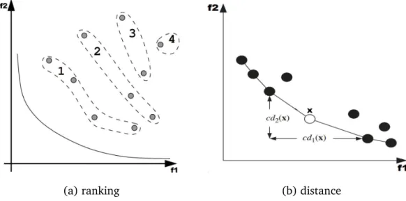
3.6 Non-dominated sorting and crowding distance methods used in NSGA-II for two objectives (Deb et al.,2002). . . 47
3.7 Cell-based selection method in PESA-II (Corne et al.,2001). . . . 54
3.8 A classification of performance metrics (adapted fromDurillo et al.
(2011)). . . 60
3.9 Example illustration of the generational distance (GD) metric (adapted fromCoello et al. (2007)). . . 61
3.10 Example illustration of the inverted generational distance (IGD) metric. . . 62
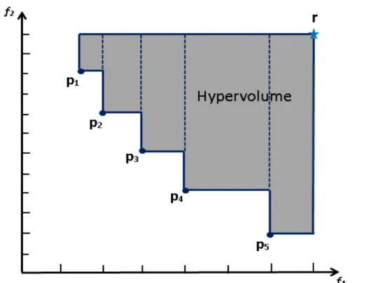
3.11 Graphical illustration of the hypervolume (HV) metric for a bi-objective minimization problem. . . 64
4.1 Example of an initial population and probability vector. . . 75
4.2 Comparison of heuristic efficient frontiers for constrained problem. 92
4.2 Comparison of heuristic efficient frontiers for constrained problem. 93
4.2 Comparison of heuristic efficient frontiers for constrained problem. 94
4.3 Mean performance of the algorithms for constrained problem. . . 95
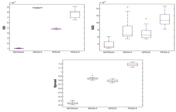
5.1 Performance comparisons of the algorithms in terms of GD, IGD and Spread (∆) metrics for Hang Seng. . . 115
5.2 Performance comparisons of the algorithms in terms of GD, IGD and Spread (∆) metrics for DAX 100. . . 115
5.3 Performance comparisons of the algorithms in terms of GD, IGD and Spread (∆) metrics for FTSE 100. . . 116
5.4 Performance comparisons of the algorithms in terms of GD, IGD and Spread (∆) metrics for S&P 100. . . 116
5.5 Performance comparisons of the algorithms in terms of GD, IGD and Spread (∆) metrics for Nikkei. . . 117
5.6 Running time of the algorithms for the constrained portfolio opti-mization problem. . . 117
5.7 Comparison of obtained Efficient Frontier of all the algorithms for constrained portfolio optimization problem. . . 118
5.7 Comparison of obtained Efficient Frontier of all the algorithms for constrained portfolio optimization problem. . . 119
5.7 Comparison of obtained Efficient Frontier of all the algorithms for constrained portfolio optimization problem. . . 120
6.1 Effectiveness of the learning-guided solution generation scheme and archive. . . 137
6.2 Performance comparisons of five algorithms in terms of GD, IGD and Diversity (∆) metrics for Hang Seng dataset. . . 140
6.3 Performance comparisons of five algorithms in terms of GD, IGD and Diversity (∆) metrics for DAX 100 dataset. . . 141
6.4 Performance comparisons of five algorithms in terms of GD, IGD and Diversity (∆) metrics for FTSE 100 dataset. . . 142
6.5 Performance comparisons of five algorithms in terms of GD, IGD
and Diversity (∆) metrics for S & P 100 dataset. . . 143
6.6 Performance comparisons of five algorithms in terms of GD, IGD and Diversity (∆) metrics for Nikkei dataset. . . 144
6.7 Performance comparisons of five algorithms in terms of GD, IGD and Diversity (∆) metrics for S & P 500 dataset. . . 145
6.8 Performance comparisons of five algorithms in terms of GD, IGD and Diversity (∆) metrics for Russell 2000 dataset. . . 146
6.9 Performance comparisons of five algorithms in terms of HV metric. 147 6.10 Comparison of efficient frontiers for seven datasets. . . 148
6.10 Comparison of efficient frontiers for seven datasets. . . 149
6.10 Comparison of efficient frontiers for seven datasets. . . 150
6.10 Comparison of efficient frontiers for seven datasets. . . 151
6.11 Comparisons of convergence of five algorithms. . . 152
6.11 Comparisons of convergence of five algorithms. . . 153
7.1 The historical VaR of feasible portfolios comprising of three stocks (Coca-Cola Co., 3M Co. and Halliburton Co.) with 3 years of data and 99% confidence interval. w1is the proportion of investment in Coca-Cola,w2 is the proportion of investment in Halliburton. The amount investment in 3M is equal to1−w1−w2. Short selling is not allowed. . . 164
7.2 Performance of algorithms in terms of IGD, HV and computational time for S & P 100. . . 174
7.3 S & P 100: Comparison of obtained efficient frontiers of each algo-rithm together with the best known optimal front obtained from all tested algorithms. . . 175
7.3 S & P 100: Comparison of obtained efficient frontiers of each algo-rithm together with the best known optimal front obtained from all tested algorithms. . . 176
7.3 S & P 100: Comparison of obtained efficient frontiers of each algo-rithm together with the best known optimal front obtained from all tested algorithms. . . 177
7.4 S & P 100: Transaction map for portfolio risk. . . 178
7.4 S & P 100: Transaction map for portfolio risk. . . 179
7.5 Performance of algorithms in terms of IGD, HV and computational time for S & P 500. . . 180
7.6 S & P 500: Comparison of obtained efficient frontiers of each algo-rithm together with the best known optimal front from all tested algorithms. . . 181
7.6 S & P 500: Comparison of obtained efficient frontiers of each algo-rithm together with the best known optimal front from all tested algorithms. . . 182
7.6 S & P 500: Comparison of obtained efficient frontiers of each algo-rithm together with the best known optimal front from all tested algorithms. . . 183
7.7 Comparison of convergence of algorithms for S & P 100. . . 185
A.1 Performance comparisons of five algorithms in terms of GD, IGD and Diversity (∆) metrics for Hang Seng dataset withK= 5. . . . 223 A.2 Performance comparisons of five algorithms in terms of GD, IGD
and Diversity (∆) metrics for DAX 100 datasetK= 5. . . . 224 A.3 Performance comparisons of five algorithms in terms of GD, IGD
and Diversity (∆) metrics for FTSE 100 datasetK= 5. . . . 224 A.4 Performance comparisons of five algorithms in terms of GD, IGD
and Diversity (∆) metrics for S & P 100 datasetK= 5. . . . 225 A.5 Performance comparisons of five algorithms in terms of GD, IGD
and Diversity (∆) Metrics for Nikkei datasetK= 5. . . . 225 A.6 Performance comparisons of five algorithms in terms of GD, IGD
and Diversity (∆) metrics for S & P 500 datasetK= 5. . . . 226 A.7 Performance comparisons of five algorithms in terms of GD, IGD
and Diversity (∆) metrics for Russell 2000 datasetK= 5. . . . . 226 A.8 Performance comparisons of five algorithms in terms of GD, IGD
and Diversity (∆) metrics for Hang Seng datasetK= 15. . . . 227 A.9 Performance comparisons of five algorithms in terms of GD, IGD
A.10 Performance comparisons of five algorithms in terms of GD, IGD and Diversity (∆) metrics for FTSE 100 datasetK= 15. . . . . . 228 A.11 Performance comparisons of five algorithms in terms of GD, IGD
and Diversity (∆) metrics for S & P 100 datasetK= 15. . . . 229 A.12 Performance comparisons of five algorithms in terms of GD, IGD
and Diversity (∆) metrics for Nikkei datasetK= 15. . . . 229 A.13 Performance comparisons of five algorithms in terms of GD, IGD
and Diversity (∆) metrics for S & P 500 datasetK= 15. . . . 230 A.14 Performance comparisons of five algorithms in terms of GD, IGD
2.1 The benchmark instances from OR-library. . . 23
4.1 Parameter settings of PBILDE, DE and PBIL. . . 84
4.2 Comparison results of PBILDE with DE and PBIL for the uncon-strained problem. . . 86
4.3 Comparison results of PBILDE with Chang et al. (2000) and Xu et al.(2010) for the unconstrained problem. . . 87
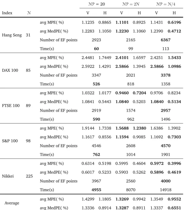
4.4 Comparison results of PBILDE with different population size (NP) for the constrained problem. . . 88
4.5 Comparison results of PBILDE with and without partially guided mutation. . . 89
4.6 Comparison results of PBILDE with and without elitism. . . 90
4.7 Comparison results of PBILDE with population size (NP) = N/4 against DE and PBIL for the constrained problem. . . 91
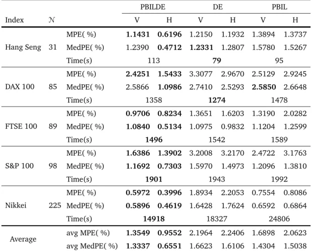
4.8 Comparison results of PBILDE against other existing algorithms (Chang et al.,2000;Xu et al.,2010) for the constrained problem. 96
4.9 Comparison results of PBILDE against Gaspero et al. (2011) and
Fern´andez and G´omez(2007) for the constrained problem. . . . 98
4.10 Comparison results of our Hybrid Algorithm(PBILDE) against Woodside-Oriakhi et al (Woodside-Oriakhi et al.,2011) for the constrained problem. . . 99
5.1 Parameter setting of considered algorithms. . . 114
5.2 Student t-Test Results of Different Algorithms on five problem in-stances from OR-Library. . . 121
6.1 How correlation effects co-movement of assets and risk. . . 133
6.2 Parameter setting of five algorithms. . . 139
6.3 Student’s t-test results of different algorithms on seven problem instances withK= 10,ǫi = 0.01,δi = 1.0,z30= 1and ϑi = 0.008. 154 6.4 Student’s t-test results of different algorithms on 5 problem
in-stances withK= 15,ǫi = 0.01,δi = 1.0,z30 = 1and ϑi = 0.008. . 155 6.5 Student’s t-test results of different algorithms on five problem
in-stances withK= 5,ǫi = 0.01,δi = 1.0,z30= 1and ϑi = 0.008. . . 155
7.1 Parameter Setting of the Algorithms. . . 173
7.2 Student’s t-Test Results of Different Algorithms on S & P100 dataset.184
7.3 Student’s t-Test Results of Different Algorithms on S & P 500 dataset.185
8.1 Summary of the algorithms with considered constraints. . . 188
B.2 Example data for first five assets of Hang Seng dataset (D1). . . . 231
B.3 Example of daily financial time series data for three assets over a period of 750 trading days. . . 232
B.4 List of 94 Securities of S & P 100 . . . 233
Acronyms
CLA Critical Line Algorithm
DE Differential Evolution
DEMO Differential Evolution for Multi-objective Optimization
EA Evolutionary Algorithm
EDA Estimation of Distribution Algorithm
EF Efficient Frontier ES Expected Shortfall GA Genetic Algorithm GD Generational Distance HC Hill Climbing HV Hypervolume
IBEA Indicator-based Evolutionary Algorithm
IGD Inverted Generational Distance
MA Memetic Algorithm
MIQP Mixed Integer Quadratic Programming
MODE Multi-objective Differential Evolution MOEA Multi-objective Evolutionary Algorithm
MOEA/D Multi-objective Evolutionary Algorithm with Decomposition MOP Multi-objective Optimization Problems
MV Mean-Variance
NSGA Nondominated Sorting Genetic Algorithm NSGA-II Elitist Nondominated Sorting Genetic Algorithm PAES Pareto Archived Evolutionary Strategy
PSO Particle Swarm Optimization
PSP Portfolio Selection Problem
QP Quadratic Programming
SA Simulated Annealing
SOEA Single Objective Evolutionary Algorithm SPEA Strength Pareto Evolutionary Algorithm
SPEA2 Improved Strength Pareto Evolutionary Algorithm
SS Scatter Search
TS Tabu Search
UCEF Unconstrained Efficient Frontier
VaR Value-at-Risk
VEGA Vector Evaluated Genetic Algorithm Roman Symbols
Asize Archive size
B Reference set size
CR Crossover probability
F Amplification factor
K Number of assets in a portfolio
LR Learning rate
MP Mutation Probability
MR Mutation Rate
M Number of asset class
NP Number of individuals in a population
N Number of available assets
N LR Negative learning rate
Introduction
“Great stocks are extremely hard to find. If they weren’t, then everyone would own them.”
Philip A. Fisher
1.1
Background and Motivation
From the financial point of view, a portfolio is a collection of investments held by an individual or a financial institution. These investments can be financial assets ranging from stocks, bonds, or options to real estate. In financial mar-kets, there exists a huge variety of asset classes in which one may invest his/her wealth. Different assets have different levels of risk. Different investors have their own attitude towards the risk. Given an extensive range of financial assets with different characteristics, the essence of the problem is to find a combination of assets that serves the best for an investor’s needs.
In 1952, Markowitz addressed a fundamental question in financial decision mak-ing: How should an investor allocate his/her wealth among the possible in-vestment choices? Markowitz introduced a parametric optimization model by proposing that investors should decide the allocation of their investments based on a trade-off between risk and return. Markowitz’s mean variance (MV) model
proposes that investment returns can be represented by a weighted average of the returns of the underlying assets and risk is reflected as the variability of payoffs. Markowitz’s mean variance (MV) principle (Markowitz, 1952, 1959) is considered to play an important role in the development of modern portfolio theory.
Many investment situations may make investment managers consider MV frame-work for wealth allocation. Based on market index historic returns, an tional equity manager may need to find optimal asset allocations among interna-tional equity markets. A plan sponsor may like to find an optimal long-term in-vestment policy for allocating among different classes such as domestic, foreign bonds and equities. A domestic equity manager may wish to find an optimal equity portfolio based on forecasts of return and estimated risk (Michaud and Michaud,2008).
MV optimization model is useful as an asset management tool for many applica-tions, such as (Michaud and Michaud,2008):
• Implementing investment objectives and constraints
• Controlling the components of portfolio risk
• Implementing the asset manager’s investment strategies
• Using active return information efficiently
• Embedding new information into portfolios efficiently
Moreover, the MV optimization model is flexible enough to reflect various prac-tical trading constraints and it can thus be served as the standard optimization framework for modern asset management (Michaud and Michaud,2008). There are exact methods such as simplex methods (Dantzig,1998), interior point methods (Adler et al.,1989) and quadratic programming methods (Hirschberger et al.,2010;Markowitz,1987;Stein et al.,2008) which can be employed in order
to find the optimal solution for the basic MV model with a reasonable compu-tational effort. However, these methods can be applied to problems satisfying certain conditions such as the objective function must be of a certain type, the constraints must be expressible in certain formats, and so on (Boyd and Vanden-berghe,2004). Without modifying and/or simplifying the problems into solvable forms, the applications of these methods are therefore limited to a certain set of problems (Maringer,2005).
The basic MV framework for portfolio optimization assumes markets to be fric-tionless. In real market, investors commonly face real-world trading restrictions and it requires that the constructed portfolios have to meet trading constraints. Investors also have their own preferences and this may lead to impose further constraints in allocating capital among the assets. It is therefore needed to ex-tend the standard model in order to reflect practical trading restrictions and investors’ valuable insights.
When additional constraints are added to the basic MV model, the problem thus becomes more complex and the exact optimization approaches run into difficulties to deliver solutions within reasonable time for large problem size. By introducing the cardinality constraint alone already transformed the clas-sic quadratic optimization model into a mixed-integer quadratic programming problem which is an NP-hard problem (Bienstock, 1996;Moral-Escudero et al.,
2006;Shaw et al.,2008). As a result, this motivates the investigation of approx-imate algorithms such as metaheuristics (Gendreau and Potvin, 2010; Glover and Kochenberger,2003) and hybrid meta-heuristics (Raidl,2006;Talbi,2002). In general, metaheuristics cannot guarantee the optimality of the solution, but they are efficient in finding the optimal or near optimal solutions in a reasonable amount of time.
Markowitz (1959) also noted that risk quantification for portfolio optimization is an open problem since it depends on the investor’s needs. No one risk mea-sure, therefore, may satisfy different needs of different investors. Many stud-ies have been conducted to quantify the portfolio risk with different measures.
A particular class of measure which quantify possibilities of return below ex-pected return are called downside risk measures (Harlow,1991;Krokhmal et al.,
2011). Among those downside risk measures, Value-at-Risk (VaR) (Morgan,
1996) is a popular measurement of risk widely recognized by financial regu-lators and investment practitioners. The portfolio optimization in the VaR con-text involves additional complexities since VaR is non-linear, non-convex and non-differentiable, and it exhibits multiple local extrema and discontinuities es-pecially when real-world trading constraints are incorporated (Gaivoronski and Pflug, 2005). In fact Benati and Rizzi (2007) show that optimization of the mean-VaR portfolio problem leads to a non-convex NP-hard problem which is computationally intractable.
In the past decade, there has been an increasing interest to explore the appli-cation of evolutionary algorithms for portfolio optimization problems. Evolu-tionary algorithms, a class of metaheuristics, are one of the known alternatives for optimization problems that are too complex to be solved using deterministic techniques. They are independent of the types of objective function and the con-straints while also being attractive for their capability to solve computationally demanding problems reliably and efficiently.
The motivation for this thesis is based on three main avenues in the literature on portfolio optimization. The first area of interest is to design hybrid evolutionary algorithms for portfolio optimization problems. In particular, we are interested in integrating selective properties of different evolutionary approaches in order to mitigate their individual weaknesses and achieve efficient convergence of the search. The second area of interest is to extend the basic model with practi-cal trading constraints in order to better reflect the practipracti-cal trading limitations. Recent review by Metaxiotis and Liagkouras (2012) shows that the cardinality and quantity constraints are the most commonly considered constraints in the literature. Therefore, we are interested in investigating the portfolio optimiza-tion models as realistic as possible by considering increasing number of practical trading constraints. The third area of interest is to adopt VaR as an alternative risk measure in place of the variance. Recent surveys by Metaxiotis and
Liagk-ouras (2012) andPonsich et al. (2013) also show that the research in portfolio optimization in the nonparametric mean-VaR framework is still in its infancy compared to mean variance framework.
1.2
Aims and Objectives
The goal of this thesis is to provide a contribution to portfolio optimization re-search through the development of efficient and effective algorithms and to in-vestigate their applications to portfolio optimization problems with additional practical trading constraints. In order to achieve this goal, the identified objec-tives are as follows:
• To extend the basic portfolio model as realistic as possible by considering increasing number of practical trading constraints.
• To design and investigate the ability of single objective evolutionary algo-rithms to deliver high-quality solutions for the constrained portfolio opti-mization problems.
• To design effective and efficient multi-objective evolutionary algorithms for portfolio optimization problems reflecting practical trading constraints.
• To conduct a fair performance comparison between the proposed algo-rithms and existing state-of-the-art evolutionary algoalgo-rithms.
• To investigate an alternative industry standard risk measure for the port-folio optimization problems in order to capture the asymmetric nature of risk.
1.3
Contributions
The contributions of this thesis can be summarized as follows:
• A hybrid evolutionary algorithm (PBILDE) is developed to solve the port-folio optimization problems with cardinality and quantity constraints (see
Chapter4). A partially guided mutation and an elitist update strategy are proposed in order to promote the efficient convergence of PBILDE. PBILDE is able to achieve a strong synergetic effect through hybridization of PBIL and DE. In most problem instances, it also outperforms other existing ap-proaches in the literature which adopted the same mean variance model.
• A multi-objective scatter search with external archive (MOSSwA) algorithm is proposed for the first time for portfolio optimization problems with cardi-nality, quantity and pre-assignment constraints (see Chapter5). MOSSwA adapts the basic scatter search template to multi-objective optimization by incorporating the concepts of Pareto dominance, crowding distance and elitism. New subset generations and solution combination methods are proposed to generate efficient and diverse portfolios. MOSSwA outper-forms NSGA-II, SPEA2 and PESA-II in all five problem instances both in terms of solution quality and computational time.
• A learning-guided multi-objective evolutionary (MODEwAwL) algorithm is developed to solve the portfolio optimization problems with cardinality, quantity, pre-assignment and round lot constraints (see Chapter 6). A learning mechanism is introduced in order to extract important features from the set of elite solutions. Problem-specific selection heuristics are introduced in order to identify high-quality solutions with a reduced com-putational cost. An efficient and effective candidate generation scheme utilizing a learning mechanism, problem specific heuristics and effective direction-based search methods is proposed to guide the search towards the promising regions of the search space. In small problem instances, MODEwAwL is competitive to NSGA-II and SPEA2. In large problem in-stances, MODEwAwL achieves better performance over four existing well-known MOEAs, NSGA-II, SPEA2, PEAS-II and PAES. The computational re-sults not only show that the quality of the generated solutions significantly improved, but also that the overall computation time can be reduced.
• Value-at-risk (VaR), an industry standard risk measure, is studied in order to reflect a realistic risk measure. The mean-VaR portfolio optimization
problem with six practical constraints is for the first time considered (see Chapter 7). A multi-objective evolutionary algorithm with guided learn-ing (MODE-GL) is developed to solve the constrained mean-VaR portfolio optimization problems. Two different variants of DE mutation schemes in the solution generation scheme are proposed in order to promote the explo-ration of the search towards the least crowded region of the solution space. When the cardinality constraints are considered, incorporating a learning mechanism significantly promotes the efficient convergence of the search.
1.4
Outline
The structure of this thesis can be summarized as follows. Chapter2provides an introduction to the background of the thesis, through a brief overview of variants of optimization approaches for the single-period portfolio optimization models. A number of practical constraints commonly faced by investors and datasets uti-lized for computational analysis in this thesis are also described. Chapter3 pro-vides an overview of the key concepts in multi-objective optimization problems. Most well-known population-based evolutionary algorithms are reviewed and their applications are summarized.
Chapter 4 presents a hybrid algorithm for portfolio optimization problem with cardinality and quantity constraints and investigates the effectiveness of the com-ponents of the algorithm. Chapter 5 describes a multi-objective scatter search algorithm for portfolio optimization problems with three constraints. Chapter6
presents a learning-guided multi-objective evolutionary algorithm for the mean variance portfolio optimization problems. Chapter 7 studies the Value-at-Risk (VaR) as an alternative risk measure and presents a multi-objective evolutionary algorithm with guided learning for mean-VaR portfolio optimization problems. Chapter8 concludes with a summary and suggestions for future research direc-tions.
Portfolio Optimization
“It’s not whether you’re right or wrong that’s important, but how much money you make when you’re right and how much you lose when you’re wrong.”
George Soros
2.1
Introduction
Portfolio optimization plays an important decision making role in investment management. It is concerned with the optimal allocation of a limited capital among a finite number of available assets, such as stocks, bonds and deriva-tives, in order to gain the highest possible future return subject to a tolerance level at the end of the investment period. Mean-variance portfolio formulation (Markowitz, 1952, 1959) pioneered by Nobel Laureate Harry Markowitz has provided an influential insight into decision making concerning the capital in-vestment in modern computational finance. Since the return of the inin-vestment is not guaranteed but approximated (i.e., expected), a variation of the return should be considered as the risk of receiving the expected return. Markowitz therefore reasoned that investors should not only be concerned with the realized returns, but also the risk associated with the asset holdings and introduced the
portfolio optimization as a mean variance optimization problem with regard to two criteria: to maximize the reward of a portfolio (measured by the mean of expected return), and to minimize the risk of the portfolio (measured by the variance of the return). In the simplest sense, a desirable portfolio is defined to be a trade-off between risk and expected return.
This chapter provides an introduction to the background of the thesis, through a review of the relevant portfolio optimization problems with different approaches. A portfolio optimization model with an alternative risk measure is also described. In addition, a number of real-world trading constraints commonly faced by in-vestors are discussed. The detailed descriptions of the datasets used in this thesis for computational analysis are also presented.
2.2
Markowitz’s Mean-Variance Model
Markowitz(1952,1959) introduced a parametric optimization model in a mean variance framework which provides analytical solutions for an investor either trying to maximize his/her expected return for a given level of risk or trying to minimize the risk for a given level of expected return. The mean variance (MV) model assumes that the future market of the assets can be correctly reflected by the historical market of the assets. The reward (profit) of the portfolio is measured by the average expected return of those individual assets in the port-folio whereas the risk is measured by its combined total variance or standard deviation. Markowitz’s mean variance model (MV model) is formulated as an optimization problem over real-valued variables with a quadratic objective func-tion and linear constraints as follows:
minimize N X i=1 N X j=1 wiwjσij (2.1) subject to N X i=1 wiµi =R∗ (2.2)
N
X
i=1
wi = 1 (2.3)
0≤wi ≤1, i= 1, . . . ,N (2.4)
where N is the number of available assets, µi is the expected return of asset i (i = 1, . . . ,N), σij is the covariance between assets i and j (i = 1, . . . ,N;j =
1, . . . ,N), R∗ is the desired expected return, andw
i (0≤ wi ≤ 1) is the decision
variable which represents the proportion held of asset i. Eq. (2.1) minimizes the total variance (risk) associated with the portfolio whilst Eq. (2.2), thereturn constraint, ensures that the portfolio has a predetermined expected return of R∗. Eq. (2.3) defines the budget constraint (all the money available should be invested) for a feasible portfolio while Eq. (2.4) requires that all investment should bepositive, i.e., no short sales are allowed.
2.2.1
Single Objective Mean-Variance Model
An alternative form of the MV model can be formulated by introducing a risk aversion parameter λ∈ [0,1]to form an aggregate objective function which is a weighted combination of both return and risk as follows:
minimize λ " N X i=1 N X j=1 wiwjσij # + (1−λ) " − N X i=1 wiµi # (2.5) subject to N X i=1 wi = 1 (2.6) 0≤wi ≤1, i= 1, . . . ,N (2.7)
In Eq. (2.5), when λ is zero, the model maximizes the mean expected return of the portfolio regardless of the variance (risk). On the other hand, when λ equals one, the model minimizes the risk of the portfolio regardless of the mean
expected return. As theλ value increases, the relative importance of the return decreases, and the emphasis of the risk to the investor increases, and vice versa.
2.2.2
Multi-objective Mean-Variance Model
Mean-Variance model is considered to be the first systematic treatment of in-vestor’s conflicting objectives of higher return versus lower risk. Portfolio opti-mization problem is intrinsically a multi-objective problem since the objective is to find portfolios amongst theNassets that can simultaneously satisfy the above two conflicting objectives, i.e., minimize the total variance (see Eq. (2.8)), de-noting the risk associated with the portfolio, while maximizing its profits (see Eq. (2.9)). The portfolio optimization problem can therefore be restated as:
min f1 = N X i=1 N X j=1 wiwjσij (2.8) max f2 = N X i=1 wiµi (2.9) subject to N X i=1 wi = 1 (2.10) 0≤wi ≤1, i= 1, ...,N (2.11)
The standard model, single objective model and multi-objective model are three well-established approaches commonly adopted to solve the portfolio problem.
Chang et al.(2000) stated that the solutions for the basic portfolio optimization problem can be achieved by either solving the classic MV model (see Eqs. (2.1) to (2.4)) varying λ or solving the combined objective model (see Eqs. (2.5) to (2.7)) varying R∗. Which of these models to be selected depends on the goal of the optimization and on the capabilities of the available software packages. Most researchers commonly adopt the last two models when they use a heuristic approach (Metaxiotis and Liagkouras,2012;Ponsich et al.,2013).
2.2.3
Efficient Frontier
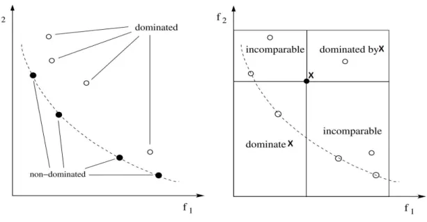
Finance theory argues that risk and expected returns are positively related, which implies that higher returns are achievable only when investors are willing to take higher risks and vice versa, i.e. the risk cannot be reduced without decreasing the return (Weigand,2014). In practice, different investors have different preferred trade-offs between risk and expected return. An investor who is very risk-averse will choose a safe portfolio with a low risk and a low expected return. Con-versely, an investor who is less risk averse will choose a more risky portfolio with a higher expected return. Thus, the portfolio optimization problem does not pre-scribe a single optimal portfolio combination that both minimizes variance and maximizes expected return. Instead, the result of the portfolio optimization is generally a range of efficient portfolios.
A portfolio is said to be efficient (i.e., Pareto optimal) in the context of mean variance portfolio optimization if and only if there is no other feasible portfolio that improves at least one of the two optimization criteria without worsening the other (see Section 3.2.1). In a two-dimensional space of risk and return, a solutionais efficient if there does not exist any solutionb such thatb dominates a(Fonseca and Fleming, 1995). Solutiona is considered to dominate solutionb if and only ifC1 orC2 holds:
C1: f1(a)≤f1(b) ∧ f2(a)> f2(b) C2: f2(a)≥f2(b) ∧ f1(a)< f1(b)
The collection of these efficient portfolios forms theefficient frontier(i.e., Pareto front) that represents the best trade-offs between the return and the risk1. We
could trace out the set of efficient portfolios by solving the model (Eqs2.5–2.7) repeatedly with a different value ofλat each time. Figure2.1shows the efficient frontier (EF) plotted in the risk-return solution space for a 31-asset universe of Hang Seng dataset from the OR-library (see Section2.5).
Figure 2.1: The unconstrained efficient frontier of 31-asset universe (Lwin and Qu,2013).
Obtaining the efficient frontier would simplify the choice of investment for in-vestors and the individual portfolios will be selected based on the investor’s risk tolerance and his/her expectation of profit in return. Well spread distribution of portfolios along the efficient frontier provides more alternative suitable choices for investors with different risk-return profiles.
2.2.4
Limitations of the Mean-Variance Model
As with any model, it is crucial to understand the limitations of mean variance analysis in order to use it effectively. Firstly, the mean variance framework was developed for portfolio construction in asingle period. In the single period port-folio optimization problem, the investor is assumed to make allocations once and for all at the beginning of an investment period, based on the risk and return es-timations and correlations of a universe ofN investable assets. Once made, the decisions are not expected to change until the end of the investment period and the impact of decisions arising in subsequent periods is not considered in this case. Hence, the mean variance model essentially represents a passive buy-and-hold strategy (Fabozzi and Markowitz,2011).
Moreover, the mean variance analysis depends on the perfect knowledge of the expected returns, standard deviation and pair-wise correlation coefficients of all assets under consideration. Chopra and Ziemba (1993) shows that the compo-sition of the optimal portfolio in the mean variance model can be very sensitive to estimation errors in problem inputs. In real world, however, real markets exhibit complexities with unknown and unobservable distributions of returns. Perfect estimates of these inputs are extremely hard, if not impossible, to obtain. Estimating these unknown parameters with free of estimation errors is a whole subject in itself and the mean variance analysis does not address this issue explic-itly. Instead, the mean variance model assumes that input parameters provide a satisfactory description of the asset returns. In particular, the first two moments of the distribution (i.e., mean and variance) are considered to be sufficient to correctly represent the distribution of the asset returns and the characteristics of the different portfolios (Crama and Schyns,2003).
Although Markowitz’s mean variance model plays a prominent role in financial theory, direct applications of this model are not of much practical uses for var-ious reasons. It implicitly assumes that the return of assets follows a Gaussian distribution (normal distribution) and investors act in a rational or risk-averse manner. A risk-averse investor prefers the investment with a lower overall risk over the one with a higher overall risk when given two different investments with the same expected return (but different risks). Finally, the model is sim-plified to be solvable under unrealistic assumptions. Thus, the basic Markowitz model does not reflect the restrictions (constraints) faced by real-world investors (Maringer,2005). It assumes a perfect market2without taxes or transaction costs where short sales are not allowed, and securities are infinitely divisible, i.e. they can be traded in any (non-negative) fraction. It is also assumed that investors do not care about different asset types in their portfolios (Vince, 2007, Chapter 7). These limitations have consequently motivated further developments to improve its applicability in real-world (see Section2.3.1).
2A market is considered to beperfectif and only if every possible combination of allocation of assets in a portfolio is attainable.
2.3
An Alternative to Mean-Variance Model
The mean variance analysis reflects risk as the variance or standard deviation of a portfolio. Variance is a statistical measure of the dispersion of returns around the arithmetic mean or average return (the average of squared deviations from the mean). Risk in this context can be described as an indicator of how fre-quently and by how much the true portfolio return is likely to deviate from its mean. This measure of risk is not practical because the risk of obtaining a result that is above average is considered in the same way as the risk of obtaining a result that is below average. In reality, rational investors’ perception against risk is skewed (not symmetric around the mean) as they are more concerned with under-performance rather than over-performance in a portfolio. Variance as a risk measure has thus been widely criticized by practitioners due to its symmet-rical measure by equally weighting desirable positive returns against undesirable negative ones (Grootveld and Hallerbach,1999). This gives rise to research di-rections where realistic risk measures are used to separate undesirable downside movements from desirable upside movements (Biglova et al., 2004). Among those alternative risk measures which account for the asymmetric nature of risk, Value-at-Risk (VaR) (Morgan,1996) is a popular risk measure adopted by finan-cial institutions.
2.3.1
Value-at-Risk
Value at Risk (VaR) measures the maximum likely loss of a portfolio from market risk with a given confidence level (1−α) over a certain time interval. For in-stance, if a daily VaR is valued as 100,000 with 95% confidence level, this means that during the next trading day there is only a 5% chance that the loss will be greater than 100,000. The higher the confidence level, the better chances that the actual loss will be within the VaR measure. Therefore, the confidence level (1−α) is usually high, typically 95% or 99%. Formally, the VaR at confidence level (1− α) 100 % is defined as the negative of the lower α-quantile of the return distribution:
where α ∈ (0,1), R is a random portfolio return (Kim et al., 2012; Stoyanov et al.,2013).
2.3.2
Multi-objective Mean-VaR Model
Let us assume that each time t denotes a different scenario and let rit be the
observed return of asset i at time t using historical data over the time series horizonT. Letwi be the proportion of the budget invested in asseti. Given a set
ofNassets, the portfolio’s return under scenario tis estimated by:
κt(w) = N X i=1 ¯ ritwi, t= 1, . . . , T. (2.12)
Let ρt be the probability of scenario occurrence and assume all scenarios are
considered to have equal probability (i.e.,ρt = 1/T). The expected return of the
portfolio is obtained by:
µ(w) = T
X
t=1
κt(w)ρt (2.13)
The VaR at a given confidence level (1−α) is the maximum expected loss that the portfolio will not be exceeded with a probabilityα:
ψ(w) = V aRα(w) = −inf ( κtα(w)| tα X j=1 ρj ≥α ) (2.14)
where returnsκt(w)are placed in an ascending order such thatκ(1)(w)≤κ(2)(w)≤
...≤κ(T)(w)(Anagnostopoulos and Mamanis,2011a). The negative sign is used
in Eq. (2.14) to denote the expected loss since κt(w) represents the expected return.
The mean-VaR portfolio selection problem is summarized as follows: min ψ(w) max µ(w) s.t N X i=1 wi = 1, 0≤wi ≤1 (2.15)
2.4
Real-world Constraints
The standard mean variance model is based on several simplifying assumptions. The basic model assumes a perfect market where securities are traded in any (non-negative) fractions, there is no limitation on the number of assets in the portfolio, investors have no preference over assets and they do not care about different asset types in their portfolios. In practical investment management, however, a portfolio manager often faces a number of constraints on his/her in-vestment portfolio for various reasons, such as legal restrictions, institutional fea-tures, industrial regulations, client-initiated strategies and other practical mat-ters (Skolpadungket et al., 2007). For example, a portfolio manager may face restrictions on the maximum capital allocation to a particular industry or sec-tor. As a result, the basic model can be extended with a number of real-world constraints to better reflect practical applications. In this section, we describe constraints that are often used in practical applications.
2.4.1
Cardinality Constraint
In the standard model, proportions of assets are not limited no matter how small allocation of the investment is. Very often in practice, investors prefer to have a limited number of assets included in their portfolio since the management of many assets in the portfolio is tedious and hard to monitor. They also intend to reduce transaction costs and/or to assure a certain degree of diversification by limiting the number of assets (K) in their portfolios (Skolpadungket et al.,2007).
Cardinality constraint limits the number of assets that compose the portfolio: N
X
i=1
si =K, (2.16)
where binary decision variablessi(i = 1, . . . ,N)are introduced to indicate if as-seti is included in the portfolio. Kis a positive integer less than the number of assets in the investment universe (N).
In the literature, there are two variants of cardinality constraint. One variant is the equality constraint as noted in Eq. (2.16) where cardinality constraint imposes the number of securities in the portfolio to be exactly K (Armananzas and Lozano, 2005; Chang et al., 2000, 2009; Cura, 2009; Deng et al., 2012;
Fern´andez and G´omez, 2007; Golmakani and Fazel, 2011; Jobst et al., 2001;
Skolpadungket et al., 2007; Soleimani et al., 2009; Woodside-Oriakhi et al.,
2011). Another variant is inequality constraint (i.e., N P i=1 si ≤ KorKL ≤ N P i=1 si ≤
KU) where cardinality constraint is relaxed with lower and/or upper bounds [KL,KU] (Anagnostopoulos and Mamanis,2011b;Cesarone et al.,2013;Chiam et al., 2008; Crama and Schyns,2003;Gaspero et al.,2011;John,2014; Liagk-ouras and Metaxiotis, 2014; Maringer and Kellerer, 2003; Schaerf, 2002). Al-ternatively, cardinality constraint can be addressed as one of the minimization objectives in the portfolio optimization problem. Anagnostopoulos and Mamanis
(2010) consider the portfolio optimization problem as a tri-objective optimiza-tion problem in order to achieve the trade-offs between risk, return and the number of securities in the portfolio.
2.4.2
Floor and Ceiling Constraints
The floor and ceiling constraints specify the minimum and maximum limits on the proportion of each asset that can be held in a portfolio (Chang et al.,
2000). The former prevents excessive administrative costs for very small hold-ings, which have negligible influence on the performance of the portfolio, while the latter rules out excessive exposure to a specific asset and, in some cases, it
is restricted by institutional policies. The floor and ceiling constraints are also known as bounding or quantity constraints. Using finite lower and upper bounds, ǫi andδi respectively, and the binary variablesi, the floor and ceiling constraints
can be represented as follows:
si =
(
1 iftheith (i= 1, . . . ,N) asset is held
0 otherwise, (2.17)
ǫisi ≤ wi ≤ δisi, i= 1, . . . ,N, (2.18)
Since budget constraint of the basic model requires all weights to sum up to one (see Eq. (2.3)), the sum of lower bounds should not be above one,
N
P
i=1
ǫi ≥ 1,
and the sum of upper bound should not be below 1, N
P
i=1
δi ≤ 1. Since short sales
are not allowed in the basic model, floor constraints override Eq. (2.4).
2.4.3
Round Lot Constraint
Many real-world applications require that securities are traded as multiples of minimum lots or batches. Round lot constraint requires the number of any asset in the portfolio to be in an exact multiple of the normal trading lots (Golmakani and Fazel,2011;Lin and Liu,2008;Skolpadungket et al.,2007;Soleimani et al.,
2009;Streichert et al.,2004a,b). It overcomes the assumption of infinite divisi-bility of assets the basic model (Jobst et al., 2001). If yi represents the positive
integer variables and ϑi is the minimum tradable lot that can be purchased for
each asset, the round lot constraint can be stated as follows:
wi =yi . ϑi, i= 1, . . . ,N, yi ∈Z+ (2.19)
In the literature, round lot constraints are mainly modelled in two variants (see
this work, round lot constraint is modelled as a fraction ϑi of the total invested
portfolio wealth. In other words, the round lot constraint defined in Eq. (2.19) imposes that each weight must be the multiple of a given fraction ϑi where lot
size ϑi is uniform for all assets. This approach is also adopted by Jobst et al.
(2001) andStreichert et al.(2004a,b,c).
The inclusion of round-lot constraint may require relaxation of the budget con-straint as the total capital might not be the exact multiples of the minimum trading lot prices for various assets.
2.4.4
Pre-assignment Constraint
The pre-assignment constraint is usually used to model the investor’s subjective preferences. An investor may intuitively wish a specific set of assets (Z) to be in-cluded in the portfolio, with its proportion to be determined (Chang et al.,2000;
Di Tollo and Roli, 2008). This constraint can be modelled with binary variables zi such that assets that need to be pre-assigned in a portfolio are denoted with
one (Gaspero et al.,2011).
zi = ( 1 if i∈Z 0 otherwise, (2.20) si ≥zi, i= 1, . . . ,N, (2.21)
2.4.5
Class Constraints
In practice, investors may ideally want to partition the available assets into mu-tually exclusive sets (classes). Each set may be grouped with common features or types such as health care assets, energy assets, etc. or grouped by investors’ own intuition. Investors may prefer to select at least one asset from each class to construct a well-diversified and/or safe portfolio. Let Cm, m = 1, . . . ,M, be
M sets of asset classes that are mutually exclusive, i.e., Ci ∩Cj = ∅,∀i 6= j. Class constraint requires that at least one asset from each class are invested in a
portfolio and can be defined as follows:
si ∈Cm, m= 1, . . . ,M, (2.22)
2.4.6
Class Limit Constraints
Investors may also want to restrict on how concentrated the investment portfolio can be in a particular class or sector. Similar to the floor and ceiling constraints, class limit constraints require that the total proportion invested in each class lies between lower and upper limits specified by the investors. Let Lm be the lower
bound andUmbe the upper bound for classmthen the class limit constraints are
formulated as follows: Lm ≤
X
si∈ Cm
wi ≤ Um, m= 1, . . . ,M, (2.23)
Note that class constraints (see Section 2.4.5) can be implicitly defined by class limit constraints when a lower bound of each class is defined to be positive. In this case, at least one asset from each class is required to be included in a portfolio. Class and class limit constraints are first introduced by Chang et al.
(2000) and Anagnostopoulos and Mamanis(2011a) and Vijayalakshmi Pai and Michel(2009) consequently consider the class constraints in their work. In their studies, class constraints are implied by assuming that Lm > 0 for every class m(m= 1, . . . ,M), .
2.4.7
Transaction Costs
When an investor buys or sells securities, expenses are incurred due to brokerage costs and taxes. In general, these costs could be variable and/or proportional to the traded volume. In some cases, a variable fee proportional to the traded amount (Akian et al.,1996;Davis and Norman,1990;Dumas and Luciano,1991;
Shreve and Soner,1994) might be imposed and/or they may also come together with a fixed cost (i.e. fixed fee per transaction) (Lobo et al., 2007; Oksendal and Sulem,2002). Maringer(2005) presents four variants of transaction costs:
fixed only, proportional only, proportional with lower bound and proportional plus fixed costs. Let yi ∈ N+0 be the natural, non-negative number of asset i ∈ [1, . . . ,N]andηi be its current price When an investor faces proportional costs of
ζp and/or fixed minimum costs ofζf, the transaction cost T Ci of asseti can be
expressed as such: T Ci =
ζf , fixed cost only
ζp.yi.ηi , proportional cost only
max{ζf, ζp.yi.ηi } , proportional cost with lower limit ζf +ζp.yi.ηi , proportional plus fixed cost
(2.24)
2.4.8
Turnover and Trading Constraints
This thesis is mainly concerned with the single-period portfolio selection prob-lems. For the sake of completeness, we present variants of constraints that oc-cur in the multi-period formulation of portfolio selection problems. Crama and Schyns(2003) introduces these constraints as a variant of the single-period for-mulation. Turnover constraints define maximum trading limits pre-specified by practitioners to safeguard against excessive transaction costs between trading periods (Scherer and Martin,2005)and can be described as follows (Crama and Schyns,2003):
max(wi−w(0)i ,0)≤Bi, i= 1, . . . ,N (2.25) max(wi(0)−wi,0)≤Si, i= 1, . . . ,N (2.26)
where wi(0) denotes existing proportion of asseti prior to the portfolio construc-tion,Bi denotes the maximum purchase andSi denotes maximum sale of asseti.
quantities of assets when there are high fixed transaction costs. Trading con-straints can be expressed as follows (Crama and Schyns,2003):
wi =w (0) i ∨ wi ≥w (0) i +Bi, i= 1, . . . ,N (2.27) wi =w(0)i ∨ wi ≤wi(0)−Si, i= 1, . . . ,N (2.28)
wherewi(0)represents existing proportion of assetiin the initial portfolio,Bi and Si denote the minimum purchase and sale of assetirespectively.
2.5
Datasets
Problem instances for Mean-Variance model
Test problems based on well-known major market indices for the portfolio op-timization problems are publicly available from the OR-library (Beasley, 1990,
1999). Table2.1 shows the details of these benchmark indices and their sizes. It should be noted that, for commercial reasons, these datasets have been dis-guised, such that the identities of the assets associated to the data are not unfold. In the current literature of portfolio optimization problems, these market indices provided by the OR-library have been widely used, and are recognized as the benchmark to evaluate the performance of different computational algorithms.
Instance Origin Name Number of assets
D1 Hong Kong Hang Seng 31
D2 Germany DAX100 85 D3 UK FTSE 100 89 D4 US S&P 100 98 D5 Japan Nikkei 225 D6 US S&P 500 457 D7 US Russell 2000 1318
The first five datasets (D1 − D5) built from weekly price data from March 1992 to September 1997 and their best known optimal solutions are available at: http://people.brunel.ac.uk/~mastjjb/jeb/orlib/portinfo.html. They were first introduced byChang et al. (2000). The remaining two datasets were built based on the index tracking problem and they were first introduced by
Canakgoz and Beasley(2009). These two datasets (D6 and D7) are available at: http://people.brunel.ac.uk/~mastjjb/jeb/orlib/indtrackinfo.html. An example OR-library dataset is also provided in AppendixB.1.
The first five datasets (D1 − D5) have been used for the mean variance con-strained portfolio optimization problems considered in chapter 4and chapter5. All seven datasets (D1−D7) have been used for mean variance constrained port-folio optimization problems considered in chapter6.
It should also be noted that Cesarone et al. (2011, 2013) also provide five additional market indices: EuroStoxx50 in Europe, FTSE 100 in UK, MIBTEL in Italy, S & P 500 in USA and NASDAQ in USA. These instances built from weekly price data from March 2003 to March 2008 are publicly accessible at: http://w3.uniroma1.it/Tardella/datasets.html. However, these problem instances are not very well-known and they have not been widely used by many studies.
Problem instances for mean-VaR model
In this research, two new datasets (DS1 and DS2) were created for the mean-VaR portfolio optimization problems studied in chapter 7. These two datasets based on historical daily financial market data have been retrieved from the Yahoo! Finance3. It was observed that historical time series downloaded from this site
had some missing data points and hence those assets with missing data points were discarded. The first dataset (DS1) consists of 94 securities from the S & P 100 and covers daily financial time series data over a period of three years from
01/03/2005 to 20/02/2008, totalling 750 trading days.
The second dataset (DS2) is composed of 475 securities from the S & P 500 and covers daily financial time series data over a period of one year from 11/04/2013 to 04/04/2014, totalling 250 trading days. The datasets are available to ac-cess online at: http://www.cs.nott.ac.uk/~ktl. An example of a small set of dataset is also presented in Appendix B.2. Constituents of datasets DS1 and DS2 are provided in Table B.4 and Table B.5 respectively. These datasets have been used for mean-VaR portfolio optimization with cardinality, quantity, pre-assignment, round lot, class and class limit constraints in order to study the performance of the evolutionary algorithms considered in this work presented in chapter7.
2.6
Summary
In this chapter, we provide a detailed description of the various optimization approaches for the mean variance portfolio optimization problems. In addition, the basic concepts and limitations of the mean variance (MV) model are also discussed. An alternative risk measure, value-at-risk (VaR), for the Mean-VaR model is also described. Additionally, practical trading constraints commonly faced by investors are described. The detailed descriptions of the market indices used in this thesis for computational analysis are also presented. This chapter provides an introduction to the background of the constrained portfolio opti-mization problems considered in this thesis.
Evolutionary Algorithms: An