Factor Retention Revised:
Analyzing Current Practice and
Developing New Methods
David Goretzko
Factor Retention Revised:
Analyzing Current Practice and
Developing New Methods
Inauguraldissertation
zur Erlangung des Doktorgrades der Philosophie
an der Ludwig-Maximilians-Universität München
vorgelegt von
David Goretzko
aus Hameln
Erstgutachter: Prof. Dr. Markus Bühner
Zweitgutachter: Prof. Dr. Moritz Heene
Datum der mündlichen Prüfung: 20.05.2020
1 ABSTRACT I
1 Abstract
The present thesis consists of three studies covering different methodological decisions that have to be made when conducting exploratory factor analyses. Study 1 is a review on the current practice in psychological research and new developments concerning these methodological decisions, while both Study 2 and Study 3 focus on the issue of factor retention which is the determination of the number of factors. In Study 2, a new method -combining extensive data simulation with modern machine learning modelling - is proposed. This new approach was able to outperform common factor retention criteria in a large-scale simulation study where the number of factors, the number of manifest variables, the sample size, the loading magnitudes of primary and cross-loadings, the inter-factor correlations and the variables per factor were varied. As Study 2 focuses on the accuracy of different factor retention criteria trying to approximate the data generating process, Study 3 rather deals with the reproducibility of factor solutions. Bootstrapping is proposed as a way to assess the robustness of factor solutions against sampling error which then can be used as a proxy for replicability. Demonstrating this connection between robustness and replicability, Study 3 also shows that the new approach suggested in Study 2 has higher replication rates than other criteria and therefore seems to perform well not only for simulated data, but also on real data sets.
Since the current research practice often lacks informed decisions, especially with regard to the factor retention process (Study 1), the new factor retention criterion (Study 2) needs to be refined (different models need to be created for different data conditions) and then made available to a broad research community. Providing practitioners with an easy-to-use, yet accurate retention criterion may improve the application of EFA. Until then, bootstrapping or another way of evaluating the robustness of common factor retention criteria can be used as a confidence measure (and as a proxy for replicability) to choose the best retention criterion (and the best factor solution respectively) for a given context.
2 ZUSAMMENFASSUNG II
2 Zusammenfassung
Die vorliegende Arbeit ist aus drei Manuskripten (im Folgenden Studie 1, Studie 2 und Studie 3 genannt) aufgebaut, die verschiedene Aspekte der Exploratorischen Fakto-renanalyse (EFA) beleuchten. Bei der EFA handelt es sich um eine statistische Methode zur Untersuchung latenter Variablen, die als ursächlich für die Zusammenhangsstrukturen mehrerer manifester Variablen angenommen werden. In der den Manuskripten vorangestell-ten Einleitung wird das (multidimensionale) tau-kongenerische Messmodell der klassischen Testtheorie - im Kontext der EFA auch common factor model genannt - eingeführt und die Herausforderungen und Fallstricke der EFA-Durchführung vorgestellt. Die zentralen Aspekte bei der EFA sind dabei das Studiendesign (womit in erster Linie die Stichpro-benumfangsplanung gemeint ist), die Wahl einer Schätzmethode (Extraction Method), die Wahl einer Rotationsmethode (Rotation Method) und die Bestimmung der Faktorenanzahl
(Factor Retention).
In Studie 1 wird die aktuelle Anwendung der EFA im Rahmen eines umfangreichen Reviews untersucht und die neuesten methodologischen Entwicklungen und Erkenntnisse im Hinblick auf die vier genannten Hauptaspekte der EFA diskutiert. Die Mehrzahl (50.3%) der untersuchten EFAs basierten auf Stichproben mit mehr als400Beobachtungen, was ge-mäß verschiedener Simulationsstudien (z.B. MacCallum, Widaman, Zhang, & Hong, 1999; Mundfrom, Shaw, & Ke, 2005) als Mindeststichprobe empfohlen werden kann (da man die Höhe von Kommunalitäten und den Grad der Overdetermination, welcher der Anzahl der Items, die jedem Faktor zugeordnet werden können, entspricht, nicht unbedingt vor der Datenerhebung absehen kann). Dies könnte für eine verbesserte Praxis im Vergleich zu den Befunden von Fabrigar, Wegener, MacCallum, und Strahan (1999) zwanzig Jahre zuvor sprechen, als noch an Regeln zur Stichprobenplanung festgehalten wurde, die die benötigte Größe der Stichprobe in Abhängigkeit von der Variablenanzahl abschätzen. Im Hinblick auf die verwendeten Rotationsmethoden zeigt sich, dass vermehrt auf oblique Rotations-methoden gesetzt wird, was bereits bei Fabrigar et al. (1999) empfohlen wurde, jedoch dass beinahe nie unterschiedliche Rotationstechniken verglichen werden. Studie 1 diskutiert deshalb, welche Rotationsmethoden welche Annahmen treffen und wann sie entsprechend Anwendung finden sollten und fordert analog zu den Ausführungen von Browne (2001), dass verschiedene Rotationstechniken (falls möglich auch auf Teildatensätzen) getestet werden sollten. Außerdem werden sogenannte regularisierte Faktorenanalysen vorgestellt, welche den zusätzlichen Rotationsschritt in der EFA überflüssig machen könnten.
2 ZUSAMMENFASSUNG III
Hinsichtlich der Faktorenextraktion werden Simulationsstudien vorgestellt, die die verschie-denen Schätzmethoden vergleichen (z.B. Barendse, Oort, & Timmerman, 2015; De Winter & Dodou, 2012). Während die Hauptachsenanalyse (Principal Axis Factoring) am häufigs-ten in der aktuellen Forschung angewendet wird, argumentiert Studie 1, dass Maximum-Likelihood EFA für multivariat normalverteilte Daten und weighted-least-squares-Ansätze für ordinale Daten (speziell wenn die Anzahl der Antwortkategorien kleiner als fünf ist) - aufgrund der vorhandenen Fit-Indizes und der besseren Vergleichbarkeit mit konfirma-torischen Faktorenanalysen zur Validierung der Faktorstruktur - der Hauptachsenanalyse vorzuziehen sind. Bei der Bestimmung der Faktorenanzahl verlassen sich viele Anwender der EFA immer noch auf Methoden, die sich in zahlreichen Untersuchungen als nicht relia-bel herausgestellt haben (z.B. im Fall des Kaiser-Kriteriums, Zwick & Velicer, 1986), aber in Statistikprogrammen wieSPSS (IBM Corp., 2019) die Standardeinstellung sind. Da die Parallelanalyse (Horn, 1965), die unter anderem aufgrund der Robustheit gegenüber un-terschiedlichen Verteilungen der Daten (Dinno, 2009) als bisheriger “Goldstandard” gilt, in vielen Datenbedingungen keine akkurate Bestimmung der Faktorenanzahl erlaubt und moderne Methoden nur in manchen dieser Bedingungen überlegen sind, empfiehlt Studie 1 mehrere Kriterien (wenn möglich auf Teildatensätzen) zu vergleichen.
Neben neuen Kriterien zur Bestimmung der Faktorenanzahl existieren auch Kombi-nationsregeln, die vorgeben, wie Anwender der EFA auf Basis mehrerer dieser Methoden zu einer finalen Einschätzung der Dimensionalität kommen sollen (z.B. Auerswald & Mos-hagen, 2019). Da diese Kombinationsregeln und generell der Vergleich mehrer Methoden aufwendig und für Anwender mit Unsicherheiten (z.B. Welcher Methode ist in der spezi-fischen Situation eher zu trauen?) verbunden sind, wird in Studie 2 ein neuer Ansatz zur Bestimmung der Faktorenanzahl - genanntFactor Forest- vorgestellt. Dieser Ansatz verbin-det eine umfassende Datensimulation mit dem Training eines modernen Machine-Learning (ML) Modells, das auf Basis von Eigenschaften der empirschen Daten die korrekte
Fakto-renanzahl vorhersagen soll.
Dafür wurden in Studie 2 zunächst 500000 Datensätze simuliert, wobei die Anzahl der la-tenten Faktoren (k ∈ {1,2, ...,8}), die Anzahl der manifesten Variablen (p ∈ {4, ...,80}), die Stichprobengröße (N ∈ [200; 1000]), die Ladungshöhen (Haupt- und Nebenladungen) und die Korrelationen zwischen den latenten Variablen variierten. Anschließend wurden
181features- also Variablen, die zur Vorhersage der Faktorenanzahl verwendet werden
soll-ten - für jeden der Dasoll-tensätze berechnet. Bei diesen Variablen handelte es sich überwiegend um Größen, die die empirische Korrelationsmatrix beschreiben (Eigenwerte, Matrixnormen,
2 ZUSAMMENFASSUNG IV
etc.), da die Zerlegung der Korrelationsmatrix in eine systematische Komponente (der Teil der Varianz der manifesten Variablen, die durch die latenten Variablen erklärt wird) und eine unsystematische Komponente (unique variance) zentraler Bestandteil der EFA ist. Die aus den simulierten Datensätzen extrahierten featuresbildeten die Basis (das Trainingsset) für die Anwendung der ML-Algorithmen. Der neue Ansatz (die trainierten ML-Modelle) wurde anschließend in einer großen Simulationsstudie mit vier herkömmlichen Methoden (Parallelanalyse, Kaiser-Kriterium, Comparison Data und Empirical Kaiser Criterion) in
3204 Datenbedingungen hinsichtlich der Genauigkeit verglichen (pro Bedingung wurden 500 Replikationen durchgeführt). Dabei erzielte ein trainiertes xgboost-Modell (für den
xg-boost Algorithmus, siehe Chen & Guestrin, 2016) mit durchschnittlich 92.9% die höchste
Genauigkeit. In einem zweiten Schritt wurde das xgboost-Modell noch weiter verbessert, indem sowohl sechs Hyperparameter des Algorithmus getuned (optimiert) und die Lösung der Parallelanalyse, des Comparison Data Ansatzes und des Empirical Kaiser Criterion als zusätlichefeaturesin das Modell aufgenommen wurden. Dadurch erzielt das finale xgboost -Modell eine Genauigkeit (out-of-sample) von 99.3%. Da die Ergebnisse aus Studie 2 auf multivariat-normalverteilten Daten basieren und psychologische Forschung (und damit vie-le Faktorenanalysen) auf ordinavie-len Fragebogendaten fußt, wurde das Vorgehen aus Studie 2 auch für ordinale Daten mit vier bis sieben Antwortkategorien getestet. Der ordinaleFactor
Foresterzielte eine Genauigkeit (out-of-sample) von durchschnittlich98.5%, weshalb davon
auszugehen ist, dass der neue Ansatz bei entsprechendem Training auf passenden Daten (die Trainingsdaten müssen das Anwendungsfeld möglichst umfassend abdecken) eine sehr hohe Genauigkeit liefert und deshalb als eigenständige Methode zur Bestimmung der Fak-torenanzahl herangezogen werden kann. Die Ergebnisse dieser zusätzlichen Analyse werden im Kapitel “Additional Analyses: Ordinal Factor Forest” dieser Dissertation berichtet.
Der Factor Forest ermöglicht nicht nur eine genaue Vorhersage der Dimensionalität,
er liefert zusätzlich Schätzwerte für die Wahrscheinlichkeit verschiedener Faktoranzahlen. Dies kann als Maß für die Sicherheit gesehen werden, dass die vorhergesagte Faktorenan-zahl der wahren Dimensionalität entspricht. Herkömmliche Verfahren liefern in der Regel nur Punktschätzer für die Anzahl der Faktoren, so dass der Anwender keinen Anhaltspunkt für die Stabilität der Faktorlösung hat - bzw. dafür, ob Stichprobenbesonderheiten das Er-gebnis verzerren (sampling error). Bei entsprechender Datenlage wird die Replikation der Faktorenlösung unter Umständen zum Problem. Obwohl im Zuge der Replikationskrise viele methodische Praktiken in der Psychologie auf dem Prüfstand stehen, wird die Bestimmung der Faktorenanzahl selten vor dem Hintergrund der Replizierbarkeit gesehen (Osborne &
2 ZUSAMMENFASSUNG V
Fitzpatrick, 2012). Für eine erfolgreiche Replikation, bzw. Kreuz-Validierung mittels konfir-matorischer Faktorenanalyse, erscheint jedoch die korrekte Bestimmung der Faktorenanzahl unabdingbar. Entsprechend untersucht Studie 3 den Zusammenhang zwischen der Robust-heit der Methoden zur Bestimmung der Faktorenanzahl über Bootstrap-Stichproben hinweg und ihrer erfolgreichen Replikation. Dafür wurde mit vier verschiedenen Methoden die Fak-torenanzahl für 19 Datensätze mit Persönlichkeitsmaßen (das 10 Item Big Five Inventory von Rammstedt, Kemper, Klein, Beierlein und Kovaleva (2017), welches für eine
within-person Replikation genutzt wurde und das Big Five Structure Inventory von Arendasy
(2009), das denbetween-personReplikationskontext abbildet) bestimmt und die Robustheit dieser Lösung über100Bootstrap-Stichproben abgeschätzt. Es zeigte sich anschließend ein positiver Zusammenhang zwischen der Robustheit der Faktorenlösung und ihrer Replizier-barkeit. Während der Factor Forest und das Empirical Kaiser Criterion relativ robuste Lösungen über die Bootstrap-Stichproben hinweg lieferten und folglich höhere Repliakti-onsraten aufwiesen, zeigten die Parallelanalyse und Comparison Data geringere Robustheit und schlechtere Replizierbarkeit.
CONTENTS VI
Contents
1 Abstract I
2 Zusammenfassung II
3 General Introduction 1
3.1 Manuscripts of this Thesis . . . 2
3.2 The Common Factor Model . . . 3
3.3 Factor Retention . . . 6
3.3.1 Eigenvalues . . . 6
3.3.2 Kaiser-Guttman Rule . . . 7
3.3.3 Scree Test . . . 7
3.3.4 Minimum Average Partial (MAP) Test . . . 7
3.3.5 Parallel Analysis . . . 8 3.3.6 New Approaches . . . 10 4 Summary Study 1 10 4.1 Sample Size . . . 10 4.2 Extraction Methods . . . 11 4.3 Rotation Methods . . . 11
4.4 Factor Retention Criteria . . . 12
5 Summary Study 2 12 5.1 General Idea: The Factor Forest . . . 13
5.2 Results . . . 14
5.3 Additional Analyses: Ordinal Factor Forest . . . 15
6 Summary of Study 3 16 6.1 Results . . . 16 7 Discussion 17 7.1 Limitations . . . 23 7.2 Conclusion . . . 25 8 References 26 9 Study 1 34
CONTENTS VII
9.1 Abstract . . . 34
9.2 Introduction . . . 34
9.2.1 Theory and Purpose of EFA . . . 35
9.2.2 Recommendations of Fabrigar et al. (1999) . . . 35
9.3 Review of the Current Use of EFA . . . 37
9.3.1 Study Design (Number of Items and Sample Size) . . . 37
9.3.2 Extraction Method . . . 40
9.3.3 Rotation Method . . . 40
9.3.4 Factor Retention Criterion . . . 40
9.3.5 Studies with References to Fabrigar et al. (1999) . . . 41
9.4 Methodological Developments . . . 43
9.4.1 Study Design (Number of Items and Sample Size) . . . 43
9.4.2 Extraction Method . . . 45
9.4.3 Factor Retention Criterion . . . 47
9.4.4 Rotation Method . . . 50 9.4.5 Further Recommendations . . . 53 9.5 Summary . . . 54 9.6 References . . . 55 10 Study 2 62 10.1 Abstract . . . 62 10.2 Introduction . . . 62
10.2.1 Aim of the Study . . . 63
10.2.2 Random Forest . . . 64
10.2.3 Extreme Gradient Boosting and Automatic Gradient Boosting . . . 64
10.3 Methods . . . 65
10.3.1 Creating a Machine Learning Model as Factor Retention Criterion . 65 10.3.2 Feature Engineering . . . 66
10.3.3 Model Training . . . 67
10.3.4 Evaluation of the Machine Learning Models and four common Factor Retention Criteria . . . 68
10.4 Results . . . 69
10.4.1 Additional Conditions . . . 79
10.4.2 Feature Importance . . . 80
CONTENTS VIII
10.5.1 Hyperparameter Tuning . . . 82
10.6 Discussion . . . 83
10.6.1 Understanding the Black Box . . . 85
10.6.2 Conclusion . . . 86 10.7 References . . . 87 11 Study 3 91 11.1 Abstract . . . 91 11.2 Introduction . . . 91 11.3 Methods . . . 93 11.3.1 Data Analysis . . . 93 11.4 Results . . . 94 11.4.1 BFI-10 . . . 94 11.4.2 BFSI . . . 96
11.4.3 Robustness and Reproducibility . . . 98
11.4.4 Comparing the Criteria . . . 99
11.5 Discussion . . . 99
11.6 Conclusion . . . 101
LIST OF FIGURES IX
List of Figures
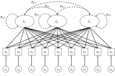
Figure 1. The common factor model with three factors and nine variables. The
arrows connecting the latent variables with the manifest variables rep-resent the respective factor loadings λij. ϕa,b indicates a possible
cor-relation between the latent factors a and b.
Figure 2. An exemplary Scree plot showing two cases - an unambiguous Scree
plot (Scree1: solid line) where obviously one factor has to be extracted and an ambiguous Scree plot (Scree2: dashed line) where no “elbow” can be detected.
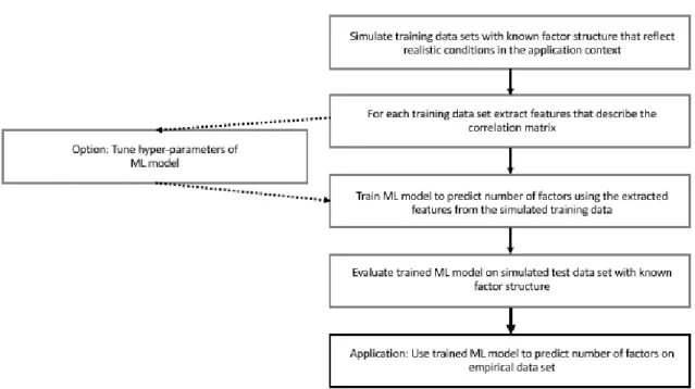
Figure 3. Visualization of the new factor retention approach (figure from Study
2).
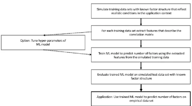
Figure 4. Study 2: Visualization of the new factor retention approach.
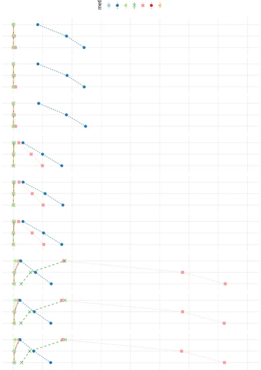
Figure 5. Study 2: Accuracy of retention criteria for conditions with one factor
averaged over N.
Figure 6. Study 2: Accuracy of retention criteria for conditions with two factors
averaged over N and ρ.
Figure 7. Study 2: Accuracy of retention criteria for conditions with four factors
averaged over N and ρ.
Figure 8. Study 2: Accuracy of retention criteria for conditions with six factors
LIST OF TABLES X
List of Tables
Table 1. Traditional Parallel Analysis: Example for Simulated Data with Ten
Variables based on Two Factors
Table 2. Study 1: Sample Sizes in EFAs in Current Psychological Research
Table 3. Study 1: Item to Factor Ratio (A) and Minimum Variables per Factor
(B)
Table 4. Study 1: Average Communalities in EFAs in Current Psychological
Re-search
Table 5. Study 1: Extraction Methods in EFAs in Current Psychological
Re-search
Table 6. Study 1: Rotation Methods in EFAs in Current Psychological Research
Table 7. Study 1: Factor Retention Criteria in Current Psychological Research
Table 8. Study 2: Accuracy of Retention Criteria averaged over All Conditions
and for Different Factor Solutions separately
Table 9. Study 2: Mean and Median Solution for each Number of Factors
Table 10. Study 2: Proportions of Under- and Overfactoring for the Different
Number of Factors
Table 11. Study 2: Accuracy of Retention Criteria for Different Sample Sizes
Table 12. Study 2: Accuracy of Factor Retention Criteria for Conditions with
Negative and Positve Loadings (A) and a Data Condition based on a Random Intercept Model (B)
Table 13. Study 2: Feature Importance: 15 Most Important Features of the
Xg-boost Model
Table 14. Study 2: Hyperparameter Space for Tuning
Table 15. Study 2: Explaining the Xgboost Model for Exemplary Data
Table 16. Study 3: Solutions of the Four Retention Criteria, Bootstrapped Means
and Standard Deviations as well as Percentages of Bootstrap Samples with the Same Factor Solution as the Respective Empirical BFI-10 Data Set
Table 17. Study 3: Solutions of the Four Retention Criteria, Bootstrapped Means
and Standard Deviations as well as Percentages of Bootstrap Samples with the Same Factor Solution as the Respective Empirical BFSI Data Set
LIST OF TABLES XI
Table 18. Study 3: Means and Medians of Standard Deviations and Rates of
Consistency over all Data Sets for the Four Retention Criteria as well
as the Means of both Replicability Measures (Dependent Variables of the GLM Analyses)
3 GENERAL INTRODUCTION 1
3 General Introduction
Exploratory factor analysis (EFA) is a statistical method commonly used in psycho-logical research to evaluate the intercorrelations among a set of observed variables and to discover underlying latent structures. The basic idea is that latent (unobservable) variables - namely psychological constructs like intelligence or personality traits - are represented by manifest variables which is known as the “common cause relation” (Reichenbach, 1956 as cited in Haig, 2005). Conversely, this means that using EFA one can find latent variables that can explain observations of a given set of manifest items. Spearman (1904) was the first to formulate the basic concept of factor analyses, followed by several researchers mainly from the field of intelligence research improving the methodology (Bartholomew, 1995). In this process, the influence of Thurstone was particularly important as he coined the terms “communality” and “uniqueness” (1940) and advocated the aim of simple structure solutions (1947). It was also Thurstone (1947) who formulated the multidimensional factor model
-also known as the common factor model which reflects the (multidimensional) congeneric measurement model that is known from classical test theory (Jöreskog, 1971).
Within the process of questionnaire development (or test construction), EFA plays a very important role. Usually, conducting several EFAs is the starting point when indicators for a specific psychological construct are evaluated and subfacets of these constructs are explored. This procedure is often entangled with the development and the refinement of theories. In personality psychology, the most prominent example for the impact of EFA on construct definition and theory development is the history of the big five trait taxonomy as described by John and Srivastava (1999). However, the relevance of EFA is not limited to personality psychology as there are application context in all psychological disciplines -i.e. intelligence research (e.g. Cohen, 1957), organizational psychology (e.g. Smith, Organ, & Near, 1983), developmental psychology (e.g. Ronald, Happé, Hughes, & Plomin, 2005), clinical psychology (e.g. Comrey, 1957) or social psychology (e.g. Marsh, Barnes, & Hocevar, 1985). Thus, EFA is arguably one of the most influential statistical methods in psychological research. However, reviews considering the application of EFA (e.g. Fabrigar et al., 1999) have shown that the actual research practice often lacks informed methodological decisions - especially with regard to selecting an extraction method, a rotation method and a factor retention criterion. As determining the number of factors is probably “the most important decision a researcher will make” (Zwick & Velicer, 1986) when conducting an EFA, this thesis pays particular attention to the factor retention process presenting new approaches
3.1 Manuscripts of this Thesis 2
that cover different of its aspects. The main focus of this work is on an innovative method that promises to be accurate, user-friendly and replicable when estimating the number of factors. As this new factor retention criterion is tailored to specific application contexts, this thesis first reviews both the current use of EFA and methodological developments in this field (with regard to all major methodological decisions in EFA).
3.1 Manuscripts of this Thesis
The following manuscripts contain the three studies this thesis is based upon: 1. Goretzko, D., Pham, T. T. H., & Bühner, M. (2019). Exploratory factor analysis:
Current use, methodological developments and recommendations for good practice.
Current Psychology. doi:10.1007/s12144-019-00300
2. Goretzko, D., & Bühner, M. (under review). One model to rule them all? Using machine learning algorithms to determine the number of factors in exploratory factor analysis.1
3. Goretzko, D., & Bühner, M. (under review). Two factors, or rather four? Robustness of factor solutions in exploratory factor analysis.
Hereafter, Study 1 refers to the first manuscript, Study 2 to the second and Study 3 to the third respectively. Study 1 is a review on the current practice and methodological developments within EFA research focusing on the major decisions a researcher has to make - which extraction method to use, which rotation method to apply and how many factors to retain. In Study 2, a new approach for determining the number of factors in EFA is proposed and evaluated, whereas Study 3 focuses the relation of robustness and replicability in factor retention.
All manuscripts were written by the author of this thesis. Markus Bühner acted as the supervising author of all three papers, while Trang T. H. Pham collected data for the review on the current use of the EFA in Study 1. The idea and conception of the studies, especially the development of the new factor retention criterion in Study 2 was generated solely by the author of this thesis. As all manuscripts were created in consultation with the 1The article was published with some minor changes after the submission of this thesis: Goretzko, D.,
& Bühner, M. (2020). One model to rule them all? Using machine learning algorithms to determine the number of factors in exploratory factor analysis.Psychological Methods. doi:10.1037/met0000262
3.2 The Common Factor Model 3
co-authors, the pronoun we is used in the summary of Study 1, Study 2 and Study 3 (as it has been done in the respective manuscripts).
After a short introduction to the common factor model and its implications for the estimation of factor loadings and factor scores as well as an introduction to the issue of factor retention, the three manuscripts are summarized and discussed.
3.2 The Common Factor Model
The common factor model assumes linear relations between each manifest variable and the k underlying latent variables. When all p manifest variables (and the latent vari-ables) are mean-centered, the common factor model for each manifest variable xi (with
i∈ {1, ..., p}) can be written as:
xi =λi1ξ1+λi2ξ2+...+λikξk+ϵi
whereξj is the j-th latent variable (or factor, where j∈ {1, ..., k}) and ϵi2 is an error
term consisting of measurement error and item-specific “uniqueness”. The common factor model for allp manifest variables combined can be written as:
x=Λξ+ϵ
with x being a vector containing all p manifest variables, ξ containing the k latent factors, ϵ containing the error terms and Λ being a p×k matrix containing the model parametersλij called factor loadings. From this, one can derive that the covariance matrix
of the manifest variables Σ=E(xx⊤)can be written as:
E(xx⊤) =E((Λξ+ϵ)(Λξ+ϵ)⊤) =E(Λξξ⊤Λ⊤) +E(Λξϵ⊤) +E(ϵξ⊤Λ⊤) +E(ϵϵ⊤)
setting E(ξξ⊤) =Φand E(ϵϵ⊤) =Ψ2, this expression becomes:
Σ=ΛΦΛ⊤+Ψ2
2Note:
3.2 The Common Factor Model 4
since E(Λξϵ⊤) = E(ϵξ⊤Λ⊤) = 0 due to the independence of ξ and ϵ. Φ is a k×k matrix containing the inter-factor correlations andΨ2is ap×pdiagonal matrix3 containing the unique variances of the manifest variables.
Figure 1 displays the common factor model for three latent variables and nine observed ones. It shows that correlations among factors are allowed, whereas correlations among error terms are not.
𝜉" 𝜉# 𝜉$ 𝑥" 𝑥# 𝑥$ 𝑥& 𝑥' 𝑥( 𝑥) 𝑥* 𝑥+ 𝜖" 𝜖# 𝜖$ 𝜖& 𝜖' 𝜖( 𝜖) 𝜖* 𝜖+ 𝜙"," 𝜙",# 𝜙",$ 𝜙#,$ 𝜙#,# 𝜙$,$
Figure 1. The common factor model with three factors and nine variables. The arrows
connecting the latent variables with the manifest variables represent the respective factor loadings λij. ϕa,b indicates a possible correlation between the latent factors a and b.
Introducing the error term ϵi and the unique variance Ψ2 respectively, the common
factor model can be distinguished from principal component analysis (PCA) which is rather a tool of dimensionality reduction than an EFA in a narrow sense. Without the underlying measurement model, PCA does not account for measurement error and the resulting com-ponents (no latent variables per se) are positively biased compared with common factors4,
yet principal component scores are determinate unlike factor scores in the common factor model (Widaman, 2007). This so-called factor indeterminacy emerges from the fact that the common factor model contains more latent than manifest variables, so independent of
3Ψ2 is a diagonal matrix since allϵ
iare independent of each other in the common factor model (i.e. no correlated errors are allowed in this measurement model).
3.2 The Common Factor Model 5
the particular sample size, infinite possible solutions are plausible for the factor scores ξ and the error terms (Steiger, 1979).
Not only determining the factor scores becomes problematic for the common factor model, but also estimating both factor loadings (λij) and unique variances simultaneously
can be challenging. A variety of extraction methods have been developed to tackle this problem with principal axis factoring (PAF, e.g. Holzinger, 1946) and Maximum-Likelihood estimation (ML, e.g. Jöreskog, 1967) being the most popular (see study 1). The objective or discrepancy functions (the functions that are minimized during the respective estimation process) reveal the differences between these two extraction methods:
FP AF = 1 2tr [(S−Σ) 2] =∑ i ∑ j (sij−σij)2 FM L=log|Σ|+ tr (SΣ−1)−log|S| −p≈ ∑ i ∑ j [(sij−σij) 2 u2 iu2j ]
withSbeing the empirical correlation matrix, Σbeing the model-implied correlation matrix andu2i being the sample unique variance of the manifest variablei. Accordingly, for the ML approach the residuals between the empirical and model-implied correlation matrix is weighted by the sample unique variances. Hence, ML weighs down “weak” variables with low communalities (high uniqueness) as described by De Winter and Dodou (2012) or MacCallum, Browne, and Cai (2007).
Both objective functions are solved iteratively5, yet the proceedings for PAF and ML are different. For PAF, initial communalities are estimated that replace the diagonal of the correlation matrixSwhich becomes a reduced correlation matrixS∗that can be decomposed via S∗ = ˆΛΛˆ⊤ with Λˆ containing the estimated factor loadings. Based on these loading
estimates, the communalities are re-estimated and the procedure continues with the next iteration until the communality estimates stabilize (for further readings, see De Winter & Dodou, 2012; Jöreskog, 2007). For the ML approach, however, no initial estimates of the communalities are necessary - both the unique variances and factor loadings are estimated directly in an iterative procedure. Jöreskog (1967) developed a computational feasible way to estimate the factor loadingsΛ given current estimates for Ψ2 and vice versa.
3.3 Factor Retention 6
Since, both approaches are not useful for (very) small sample sizes andn < p scenar-ios6, new extraction methods emerged (Hirose & Yamamoto, 2014; Jung & Takane, 2008) that are based on regularized objective functions. These new methodological developments are discussed amongst others (inter alia the differences of common rotation methods that are used to obtain an interpretable pattern matrix) in the first study of this thesis.
3.3 Factor Retention
Before it is possible to estimate the model parameters (factor loadings and unique variances), researchers conducting an EFA have to determine the number of factors that should be retained. Often no theoretical assumptions can be made and the dimensionality (number of underlying factors) has to be estimated based on the empirical data set. Hence, several so-called factor retention criteria have been developed. Since Study 2 and Study 3 focus on the issue of factor retention, the following paragraph summarizes the most common criteria (see Study 1 for their proportions in the current research) and relevant new methods. The main element of the majority of these factor retention criteria are the eigenvalues of the correlation matrix of the manifest variables.
3.3.1 Eigenvalues. The symmetric p×p correlation matrix S (or the reduced correlation matrix based on the factor modelS∗) is characterized bypeigenvalues denotedη (the number of eigenvalues is equal to the rank of the respective matrix7) andpeigenvectors
denoted x via the following transformation:
Sx=ηx , x̸= 0
which holds for all ppairs of x and η.
Accordingly, the information about the correlations among thepmanifest variables is transformed topcombinations of a scalar ηand a vectorx. The sum of the eigenvalues (of the correlation matrix) equals the number of manifest variables (∑pi ηi =p) and the ratio
ηi
∑p
iηi
= ηi
p indicates the share of item variance that can be explained by the i-th linear
combination of the p manifest variables. Hence, the higher the first eigenvalues become (and the higher this ratio gets) the less of these linear combinations (and therefore less latent factors) are needed to explain the variation of the observed variables. This is the
6
n < pscenarios are data conditions with less observations than manifest variables.
7Correlation matrices are always symmetric and positive semi-definite and therefore of full rank
3.3 Factor Retention 7
gist of most factor retention criteria - the empirical eigenvalue distribution (or eigenvalue pattern) is used to determine the number of underlying factors.
3.3.2 Kaiser-Guttman Rule. The Kaiser-Guttman rule (KG; Kaiser, 1960) is a heuristic rule that suggests to extract all factors with eigenvalues greater than one. The idea is that an eigenvalue greater than one indicates that the respective factor explains more variance than a single manifest variable does8 which is a reasonable argument on population
level, but is flawed for empirical data due to sampling error as described by Braeken and Van Assen (2017). The weak performance (especially the tendency to retain too many factors [overfactoring]) of KG on sample level has been reported in several studies (e.g. Fabrigar et al., 1999; Velicer, Eaton, & Fava, 2000; Zwick & Velicer, 1986), yet it is still the most frequently used criterion in empirical research (see Study 1) and the default in statistical programs likeSPSS (IBM Corp., 2019).
3.3.3 Scree Test. Another very popular method to determine the number of fac-tors is the Scree test by Cattell (1966). This test is based on the visual inspection of a graphical representation of the empirical eigenvalue sequence. The researcher has to detect the “elbow” in a graph plotting the eigenvalues against the number of factors (see Figure 2 for an example of the so-called Scree plot). A heavy drop of the graph indicates that the factor before the drop substantially contributes, while all following factors have little further explanatory power. This idea seems to be reasonable and may be appealing to practitioners as it has high face validity, yet the interpretation can be rather difficult (as shown in Figure 2) and could lead to subjective decisions. Although there are some ideas to objectify the procedure like the Cattell-Nelson-Gorsuch approach (e.g. Nasser, Benson, & Wisenbaker, 2002) and other non-graphical methods (e.g. Raîche, Walls, Magis, Riopel, & Blais, 2013), it is not advisable to rely on these methods as they are inferior to state-of-art factor retention criteria as well (e.g. Ruscio & Roche, 2012).
3.3.4 Minimum Average Partial (MAP) Test. The MAP test by Velicer (1976) is designed for PCA, yet often applied to EFA settings as well (see Study 1). It is based on the following statistic describing the averaged squared partial correlation after x components are partialled out:
8In cases were all manifest variables are uncorrelated, the correlation matrix becomes the identity matrix
3.3 Factor Retention 8 1 2 3 4 5 6 7 0 1 2 3 4 5
Example: Scree Test
Number of Factors
Eigen
v
alue
Figure 2. An exemplary Scree plot showing two cases - an unambiguous Scree plot (Scree1:
solid line) where obviously one factor has to be extracted and an ambiguous Scree plot (Scree2: dashed line) where no “elbow” can be detected.
M APx = p ∑ i=1 p ∑ j=1 j̸=i rxij2 p(p−1)
wherexis the number of components that is currently assessed andrxij2 is the squared correlation among the i-th and j-th variable after x components are partialled out. The summary statistic M APx is calculated forx= 0, ..., p−1and minimized to determine the
number of components that are sufficient to explain the variation of all p variables. While the MAP test performs quite well when determining the number of components in PCA (e.g. Caron, 2019; Zwick & Velicer, 1986), it is not recommended for the common factor
model (see Study 1).
3.3.5 Parallel Analysis. Parallel analysis developed by Horn (1965) compares the sequence of eigenvalues of the correlation matrix with a sequence of averaged eigenvalues fromKrandom data sets with the same sample size as the empirical data set. While in this traditional approach the mean overK random data sets is used to compare each eigenvalue
3.3 Factor Retention 9
Table 1
Traditional Parallel Analysis: Ex-ample for Simulated Data with Ten Variables based on Two Factors
Eigenvalues P Amean P A95% 3.466 1.364 1.468 2.134 1.249 1.324 0.763 1.164 1.224 0.711 1.089 1.143 0.655 1.021 1.068 0.561 0.958 1.006 0.487 0.891 0.936 0.454 0.828 0.878 0.420 0.757 0.815 0.349 0.679 0.742
Note. 1000 random data sets
were simulated for comparison. P Amean are the mean eigenvalues
based on random data and P A95%
are the 95 percentile eigenvalues based on random data that are used for comparison.
with, there are other implementations using the 95%-percentile instead. Both ideas are illustrated in Table 1. The empirical first eigenvalue is compared with the average of allK first eigenvalues of the simulated random data sets (hereK = 1000) or the95%-percentile of the respective K first eigenvalues. This is done for all p eigenvalues and factors are retained as long as the empirical eigenvalue is greater than the average or 95%-percentile of the comparison eigenvalues.
Other implementations of PA are based on eigenvalues from the reduced correlation matrix that takes the communalities into account and yet other implementations use per-muted data instead of random data to preserve the skewness of the original data. These numerous types of PA vary in their performance as simulation studies show (e.g. Auerswald & Moshagen, 2019; Lim & Jahng, 2019), so practitioners should make educated decisions
4 SUMMARY STUDY 1 10
and report which implementation they use when selecting PA as their factor retention criterion.
3.3.6 New Approaches. Although PA has become the standard criterion that is often recommended due to its quite good performance across various conditions and its robustness against distributional assumptions (e.g. Fabrigar et al., 1999 and Study 1), there are several new approaches that are superior to PA in different conditions. The three most promising are discussed in Study 1 - the hull method (Lorenzo-Seva, Timmerman, & Kiers, 2011), the comparison data (CD) approach (Ruscio & Roche, 2012) and the empirical Kaiser criterion (EKC; Braeken & Van Assen, 2017), while both CD and EKC are used for comparison in Study 2 and Study 3.
4 Summary Study 1
In addition to planning the study design (sample size, degree of overdetermination [which is the number of variables per expected factor] and the choice of indicators), three major settings have to be chosen in EFA: the number of factors (or rather which factor retention criterion to use to determine this number), the extraction method and the rotation method. Study 1 combines a review on the current use of exploratory factor analysis regarding these decisions with a discussion of new methodological developments. It can be seen as a revision of the famous review by Fabrigar et al. (1999). For reviewing the current use of EFA, two journals focusing on psychological assessment (Psychological Assessment
andEuropean Journal of Psychological Assessment) were selected and every original article9
from 2007 to 2017 reporting an EFA as a main statistical analysis was included in the review (304 reported EFAs).
4.1 Sample Size
More than half of the reported EFAs (50.3%) were conducted on samples with more than400observations (compared to 33.2% in the review of Fabrigar et al., 1999), whereas
16.4% were based on samples smaller than 200 observations (compared to 44.2% in the review of Fabrigar et al., 1999). This tendency for higher sample sizes can be seen as a sign of improving study designs in psychological research based on EFA. Since several simulation studies (e.g. Hogarty, Hines, Kromrey, Ferron, & Mumford, 2005; Mundfrom et al., 2005) 9993 studies inPsychological Assessment, issues 19(1)-29(4) and 336 studies in theEuropean Journal of
4.2 Extraction Methods 11
showed the necessity for greater samples when communalities and overdetermination are low (which you cannot rule out entirely in advance), Study 1 advocates for samples with at least 400 observations. Higher sample sizes are also desirable as model parameters and factor scores are estimated with higher precision.
4.2 Extraction Methods
The majority of reviewed EFAs used PAF (51.3%) or ML estimation (16.4%), while for22.4%of the analyses the extraction method was not reported. As no extraction method is always superior (e.g. see De Winter & Dodou, 2012 for a comparison of PAF and ML), we recommended to use a weighted least squares (WLS) approach for ordinal data with few categories (see Beauducel & Herzberg, 2006; Rhemtulla, Brosseau-Liard, & Savalei, 2012) and skewed data (Holgado–Tello, Chacón–Moscoso, Barbero–García, & Vila–Abad, 2010) and ML estimation when multivariate normality can be assumed. Both WLS and ML are implemented for confirmatory factor analyses (CFA) as well, so using these extraction methods and the respective fit indices allows for cross-validating results with CFA. PAF should be rather used in case where ML estimation produces Heywood cases, as it is less prone to such estimation problems (De Winter & Dodou, 2012). New estimation algorithms especially designed for small sample sizes (and n < p scenarios) have emerged, since these conditions can be unfeasible for both PAF and ML estimation. We discussed these new approaches focusing on the proposed regularized exploratory factor analysis by Jung and Takane (2008) and the penalized EFA by Hirose and Yamamoto (2014) which is designed for wide data (many variables) and sparse loading patterns. For psychologists though, the latter seems to be more appealing as a way to replace the additional rotation step in EFA to get an interpretable solution. Using the penalized EFA instead of common EFA with subsequent rotation as discussed in Study 1 has recently been tested empirically by Scharf and Nestler (2019).
4.3 Rotation Methods
In addition to presenting the penalized EFA (Hirose & Yamamoto, 2014) as a new way to think about rotation, we focused on the common two step approach (extracting an initial factor solution and then rotating it to improve interpretability) and presented different rotation methods within the framework of the Crawford-Ferguson family (CF; Crawford & Ferguson, 1970). The general CF complexity function which is minimized with
4.4 Factor Retention Criteria 12
regard to constraints that are inherent to the respective rotation method covers several well-known rotation methods. We briefly discussed how these different criteria focusing either on row-complexity or column-complexity (see also Browne, 2001) provide simple structure patterns or benefit cross-loadings. In this context, additional weighting approaches were also introduced.
Besides reframing common rotation methods, we debated whether and when the rotation to a predefined target (Myers, Jin, Ahn, Celimli, & Zopluoglu, 2015) is appropriate and pointed out similarities of this approach to exploratory structure equation modelling (e.g. Marsh, Morin, Parker, & Kaur, 2014). Although, our review shows that current research practice has been improved as mainly oblique rotation methods were used (over 70% of the analyzed EFAs relied to oblique rotation) compared to the review of Fabrigar et al. (1999), where orthogonalVarimaxrotation was applied in more than50%of the cases, only two studies used different methods and compared the resulting patterns which is highly recommended by several authors (Browne, 2001; Fabrigar et al., 1999). Hence, in Study 1, we strongly advocated for comparing rotation methods with regard to the stability of factor patterns and the interpretability of the final solution.
4.4 Factor Retention Criteria
The most commonly used factor retention criterion was the Kaiser-Guttman rule (55.6%), followed by the Scree test (46.4%) and parallel analysis (42.1%). While parallel analysis (PA; Horn, 1965) has become a “gold-standard” for determining the number of factors, both Kaiser-Guttman (KG; Kaiser, 1960) and the Scree test (Cattell, 1966) are seen critical (e.g. Fabrigar et al., 1999). However, new promising alternatives have been developed that are superior to PA. We discussed the advantages and disadvantages of both the hull method (Lorenzo-Seva et al., 2011) and CD (Ruscio & Roche, 2012) in detail and introduced the modern version of KG - the EKC (Braeken & Van Assen, 2017). We recommended to compare the results of different retention criteria and to consider theoretical perspectives with regard to content validity for test construction purposes.
5 Summary Study 2
Besides new stand-alone factor retention criteria like CD or EKC, combination rules for several different criteria like the one proposed by Auerswald and Moshagen (2019) have been developed over the last years. Even though these rules promise high accuracies when
5.1 General Idea: The Factor Forest 13
determining the number of factors, they seem to be rather complex and therefore not very user-friendly. Furthermore, combining different criteria may reduce the confidence in the final solution. Therefore, this thesis introduces a new criterion that achieves a high accuracy, while it promises to be easily applicable for practitioners and provides probability estimates for different factor solutions that can be understood as confidence measures.
5.1 General Idea: The Factor Forest
This new approach (working title: Factor Forest) is based on extensive data simula-tion that reflects realistic data condisimula-tions of the applicasimula-tion context and modern machine learning models that are used to predict the number of factors. The basic idea of theFactor
Forest is that a (complex) statistical model can be found that describes the relationship
between the characteristics of the empirical data set and the true number of underlying latent variables. The eigenvalues of the correlation matrix and the number of manifest variables as well as the sample size are obvious choices for the predictors of such a model. Further predictors (or features in the context of machine learning models) are developed to describe the empirical correlation matrix as EFA is based on the decomposition of the inter-item correlations.
Since modelling the relationship between these (observable) features and the (unob-servable) number of factors is not feasible without knowing the true number of factors, a data basis (consisting of numerous data sets) with known factorial structure is simulated in a first step. This data basis is created varying the true number of factors (k), the sample size (N), factor loading magnitudes (primary and cross-loadings; Λ), the number of vari-ables per factor, the inter-factor correlations (Φ) and the number of manifest variables (p). For each of the data sets for this data basis, several features are calculated (mostly features that describe the correlation matrix, e.g. different eigenvalues and matrix norms) that are later used as predictor variables in the statistical model. Afterwards, a machine learning model - the xgboost algorithm (Chen & Guestrin, 2016; Chen, He, Benesty, Khotilovich, & Tang, 2018) seems to be a good choice (see Study 2) - is trained on the simulated data (de-pending on the algorithm several hyperparameters can be tuned to improve the predictive performance). The trained model can be evaluated on new simulated test data. In Study 2, this new approach is presented in detail (see Figure 3) and its performance is compared with common criteria.
5.2 Results 14
Figure 3. Visualization of the new factor retention approach (figure from Study 2).
5.2 Results
In Study 2, we first simulated 500000 data sets that served as the data basis for the machine learning model and extracted 181 different features that were presumed to have predictive power for the true number of factors. We then trained three different machine learning algorithms (mainly with default parameter settings) on this data and evaluated their performance compared to PA, EKC, CD and KG on new simulated data. For the evaluation,3204data conditions10 were created varying the true number of factors (k), the sample sizes (N), factor loading magnitudes (primary and cross-loadings;Λ), the number of variables per factor, the inter-factor correlations (Φ) and the number of manifest variables (p) as it was done for the simulation of the data basis.
The overall accuracy (out-of-sample) of the trainedxgboostmodel was higher (92.9%) than the accuracy of all common retention criteria. When tuning six of the hyperparameters of the xgboost algorithm (and adding the other criteria as features) this performance could be further increased in a second step (99.3% out-of-sample accuracy). While all common criteria showed some kind of bias (either for one factor solutions or when the number of factors were higher), the xgboost model yielded unbiased estimates for all true values 10Using500replications per condition, in total this yielded1512000simulated data sets for the evaluation
5.3 Additional Analyses: Ordinal Factor Forest 15
of k (we evaluated k ∈ {1,2,4,6}). As the provided machine learning model is a black box model, variable importance measures (e.g. standard permutation based importance measure) and tools for interpreting the final model were introduced in Study 2 as well. The first eigenvalues (not the primary eigenvalue though) were among the most important variables in the xgboost model, but the two most important features were two inequality measures that were applied to the empirical correlation matrices - the Gini coefficient (Gini, 1921) and the Kolm measure (Kolm, 1999). We also applied the so-called local interpretable model-agnostic explanations (LIME; Ribeiro, Singh, & Guestrin, 2016) that can help to understand how the tuned model comes up with a particular prediction, although it should be carefully interpreted as it relies on local linear approximations of the far more complex model (in our example: r2= 0.235for the explaining model).
In addition to its higher accuracy compared to common retention criteria, thexgboost model can provide probability estimates for different factor solutions that can serve as confidence measures for practitioners. Since such uncertainty measures are not available with the common criteria - a new approach to assess the robustness of factor retention solutions is presented in Study 3.
5.3 Additional Analyses: Ordinal Factor Forest
In Study 2, the new approach is built on multivariate normal data (which is an as-sumption often made in the context of EFA, e.g. for ML estimation), yet psychological research data are often collected via questionnaires and therefore of ordinal nature. Accord-ingly, it was necessary to also create an ordinal implementation of the Factor Forest. The procedure was equal to the multivariate normal case (as described in Study 2) - first data was simulated (here: ordinal data11based on Gaussian copulas and binomial marginal
distri-butions with varying numbers of item categories between four and seven andπ ∈ [0.2; 0.8]) and then the tuned xgboost model was trained on the extracted features (using the same
184features including the PA, CD and EKC solution as well as the number of categories as a special feature for the ordinal data). The performance of the new approach was just slightly worse for ordinal data (overall out-of-sample accuracy of 98.5%) than for normal data as reported in Study 2. The accuracy for different values of k varied between 97.9%
11
486563 data sets (initially500000, but data sets with improper correlation matrices or errors in calcu-lating features were excluded) were simulated and randomly assigned to the training or test set (70%/30% of the data sets).
6 SUMMARY OF STUDY 3 16
(k= 3) and 99.3% (k= 1), so the Factor Forest showed promising results as a stand-alone retention criterion for ordinal data as well.
6 Summary of Study 3
While the main aim of many factor retention criteria is to approximate the data generating process as close as possible (i.e. finding the “true” number of factors), replicability should not be ignored (Osborne & Fitzpatrick, 2012; Preacher, Zhang, Kim, & Mels, 2013). In practice, when there is only one empirical data set (and splitting this data set is not an option due to a small sample size), it is difficult to predict whether the assumed number of factors (based on one or several retention criteria) is robust against sampling error and reproducible later on. Study 3, therefore, evaluates an approach to assess the robustness of factor retention solutions and its usefulness as a proxy for possible replicability.
6.1 Results
Since replicability has become an issue in psychological research, researchers con-ducting an EFA should focus especially on the factor retention process as determining the number of factors may be the most far-reaching decision with regard to a successful repli-cation of the factorial structure. Common retention criteria only provide estimates of the dimensionality, but no confidence measures (or measures of uncertainties like standard er-rors). When samples are small (and they often are as Study 1 shows) the accuracy of the criteria decreases (e.g. Study 2; Auerswald & Moshagen, 2019) as the retention process is prone to sampling error12. This hampers replicability and practitioners cannot decide how
robust an estimate for the number of factors is.
Therefore, Study 3 investigated the robustness of different factor retention criteria on empirical data via bootstrapping and examined whether the robustness across bootstrap samples can be used as a proxy for reproducibility. The new xgboost model (the Factor
Forest, see Study 2), PA, CD and EKC were compared with regard to their robustness and
their reproducibility using 19data sets consisting of personality measures (the10 Item Big
Five Inventoryby Rammstedt et al., 2017 and theBig Five Structure Inventoryby Arendasy,
12This vulnerability to sampling error can be illustrated using KG: Given, for example, an eigenvalue of
1.05on population level, values below one on sample level are very likely - especially when the sample size is small. So the Kaiser-Guttman criterion will retain less than the true number of factors just by chance very often.
7 DISCUSSION 17
2009). These data sets contain either different measurements (four time points) of the same participants or different cohorts within one study project. Accordingly, two different types of replication contexts are covered - within-subject and between-subject replication studies.
The results indicate that the xgboost model and EKC are more robust against sam-pling variations13than PA and CD and tend to reproduce the number of factors more often
(an exact replication of the number of factors for two consecutive measurement periods) and more accurately (mean absolute difference of the suggested number of factors for two consecutive measurement periods). Thexgboost model had the highest rate of replicability (61.5%), while using PA only 7.7% of the cases were exactly replicated. Although, EKC showed more robustness across the bootstrap samples than the xgboost model, its replica-tion rate was only the second best (46.2%) and the mean absolute deviation of replication attempts was higher compared with thexgboostmodel (0.615to0.385). However, a positive relation between robustness across the bootstrap samples and reproducibility was found -as both robustness me-asures were positively -associated with number of exact replications and negatively associated with the deviation from two consecutive dimensionality estimates. The respective results of our GLM analyses - even though not interpretable from a signifi-cance testing perspective - underline the relation between the robustness of factor solutions and their replicability.
7 Discussion
This thesis contains three studies that cover different aspects of EFA, but predomi-nantly focuses on the issue of factor retention. Study 1 shows that current research often relies on factor retention criteria that are either not designed for the common factor model, rather subjective or not accurate on sample level. The latter is the case for the Kaiser-Guttman rule which is meaningful on population level14, but prone to sampling error and
therefore not useful as a (stand-alone) retention criterion for empirical data. Since all com-mon (and new developed) factor retention criteria lack accuracy under some data conditions, reviews like Study 1 and large-scale simulation studies (e.g. Auerswald & Moshagen, 2019) urge practitioners to compare different criteria and to combine various estimates. This ap-13The robustness was indicated by the standard deviation across100bootstrap samples and the percentage
of bootstrap samples for which the criterion suggested the same number of factors as it did on the whole data set.
14Braeken and Van Assen (2017) describe why the eigenvalue>1rule, that is associated with a positive
7 DISCUSSION 18
proach is not new as Fabrigar et al. (1999) already suggested to compare different methods two decades ago. However, the results of Study 1 demonstrate that there is a discrepancy between methodological knowledge (presented in tutorial papers and how-to guidelines) and actual research practice. Although comparing criteria and using PA rather than, for exam-ple, KG or the Scree test is recommended, various studies were based on inappropriate methodological decisions considering the factor retention process. Hence, new approaches to this issue have to be both accurate for a great range of data conditions and easy to use, so that they will be applied by the majority of researchers conducting EFAs.
The new approach presented in Study 2 - the Factor Forest - promises to tackle both of these requirements. The tuned xgboost model showed almost perfect accuracy for multivariate normal data (Study 2) and is also applicable to ordinal data as the additional analyses reported above demonstrated. So far, the new approach combining extensive data simulation and the application of complex machine learning algorithms requires a lot of computational resources and is not yet easy to use. The final trained model can be used easily though and therefore seems to be a promising alternative for the actual research practice. Providing such a model that reflects all necessary data conditions would help practitioners with a highly accurate, objective and task-related method to determine the correct number of factors for their analyses. Accordingly, theFactor Forestcovering different trained models for different types of data should be made accessible for EFA users in the future.
As discussed in Study 2, the supervised15 learning approach (for a comparison of
su-pervised and unsusu-pervised learning, see James, Witten, Hastie, & Tibshirani, 2013) requires the simulation of a data basis that includes all important data conditions. So the trained model based on data sets that are simulated for k ∈ {1,2, ...,8} (see Study 2) is able to suggest only one- to eight-factor solutions by design. Accordingly, theFactor Forestis only applicable to data sets that are somewhat similar to those it has been trained on. Study 2 shows that the new approach performs well in data conditions that are close to those in the training set, but not included. Nevertheless, for completely new conditions (e.g. panel data with considerably more manifest variables) new training data has to be simulated and 15Supervised learning - in contrast to unsupervised learning - requires a criterion for which true values
are known. Here, a simulated data basis with known factor structure (known true number of factors) is necessary to create the machine learning (or statistical) model that can predict the number of factors based on data set characteristics. EFA itself (or the related PCA) can be assigned to unsupervised learning like clustering (e.g. Hansen & Larsen, 1996) where no target variable with known values is needed.
7 DISCUSSION 19
a new model has to be trained.
In Study 2, machine learning algorithms had to be chosen for theFactor Forest imple-mentation. The xgboostalgorithm (Chen & Guestrin, 2016) - especially when tuning six of its hyperparameters - showed the best results and nearly perfect accuracy, yet implement-ing other algorithms in further versions would be possible as well. Usimplement-ing other tree-based methods (e.g. random forest implementations like the ranger by Wright & Ziegler, 2017 as evaluated in Study 2 or thecforestby Hothorn & Zeileis, 2015 which is an implementation of a conditional random forest that promises unbiased partitioning) or kernel-based methods like support vector machines (Cortes & Vapnik, 1995), while relying on the same features as predictors will probably not be superior to the tuned xgboost model. However, selecting other/further features could help to improve the accuracy as the addition of the common retention criteria EKC, PA and CD as features in Study 2 demonstrated. The current im-plementation of theFactor Forest could be extended by features specially designed for new data conditions (like it was done for ordinal data where the number of categories served as an additional feature).
Another idea would be to use the correlation matrix itself as the input instead of creating features that describe the correlation matrix mathematically and use those features as the input for the model. This could be done applying neural networks (e.g. Cheng & Titterington, 1994) since they can handle large numbers of input variables (in this case a correlation matrix of80variables has802 = 6400entries and consists of 80×79
2 = 3160unique
bivariate correlations). The numerical value of each correlation could be directly used as the input for one input node and no feature engineering would be necessary (contrary to an implementation where a graphical representation of the correlation matrix is used as the model input and the neural network is used for image processing, see e.g. Egmont-Petersen, Ridder, & Handels, 2002). The ordering of the variables would be a severe problem for this approach, though, since the structure of a correlation matrix is completely arbitrary and the position of an item X is only determined by its position in the data set. To solve this problem, the variables could be clustered in a first step to create a correlation matrix that shows concentrations of high and low correlations or the assignment of bivariate correlations to the input nodes could be randomized and repeated several times to cover the various possible structures that can occur for the same data (this would lead to a much bigger training set).
All features extracted for Study 2, on the contrary, are independent of the positioning of the manifest variables. Therefore, this procedure seems to be meaningful and worth pursuing
7 DISCUSSION 20
in this context. Nevertheless, further research could evaluate whether the use of neural networks (using the same or an extended feature set) might be beneficial - especially with regard to an integration of different data types (ordinal data, multivariate normal data, count data, etc.) into one model.
As mentioned above, further features might improve the accuracy of the new approach for the data conditions that were assessed in Study 2, for ordinal data and for other data types that have not been evaluated yet. Although the features that describe the eigenvalue patterns seem to be predictive for all types of data, additional features could be useful for specific data conditions. In contexts where the variable distributions are highly skewed and the assumption of multivariate normality has to be questioned, features describing the joint item distribution or the marginals could be helpful. As EFA is often conducted on questionnaire data and this kind of data is prone to missing values due to item non-response (e.g. Shoemaker, Eichholz, & Skewes, 2002), missingness should also be considered during the factor retention process (for more details on the impact of missing data on factor retention, see, for example, Goretzko, Heumann, & Bühner, 2019). Thus, the proportion of missing values for each variable or the type of missing data method used to handle missingness (the default is often pairwise-deletion when calculating correlation matrices) could provide valuable information for the prediction task.
Depending on the context it would also be possible to change the loss function16 (the performance measure) which is used for the training (and evaluation) of the machine learning model. In Study 2, predicting the number of factors is framed as a classification task for which several performance measures have been developed. Ferri, Hernández-Orallo, and Modroiu (2009) compare the behavior of 18 measures for classification tasks and show which measures provide similar results and which measures differ strongly. The authors also discuss which measures are independent of prior class distributions (e.g. when the classes are highly imbalanced in the training data a classifier predicting the majority class achieves a high accuracy, yet poor values for recall or precision which correspond to sensitivity and
1−specificity in the psychological research context) which is not a problem in Study 2, but could be of interest when data conditions are not evenly distributed in the training set. Since 16The loss function describes how well the model fits the data and is therefore minimized when training
the model. In the classical regression context, the quadratic loss function (see least-squares approach) or the mean squared error (MSE) is typically used as the loss function, for example. The loss functions weigh the different aspects of model misfit differently (e.g. outlier sensitivity of quadratic loss vs. absolute loss), so changing the loss function can benefit another candidate model (or leads to different model parameters in the context of model training).
7 DISCUSSION 21
the Factor Forest is currently optimized with regard to the overall accuracy (that means
that the loss function weighs every false prediction equally - no matter if the prediction is
ˆ
k= 3orˆk= 5when the actual number of factors isk= 2), it could be meaningful to adjust
the loss function to take the ordinality17of the criterion into account. One possibility would be to define the loss as a symmetric Toeplitz matrix (e.g. Gray, 2006) with a zero diagonal, for example: L= 0 1 2 3 4 5 6 7 1 0 1 2 3 4 5 6 2 1 0 1 2 3 4 5 3 2 1 0 1 2 3 4 4 3 2 1 0 1 2 3 5 4 3 2 1 0 1 2 6 5 4 3 2 1 0 1 7 6 5 4 3 2 1 0
which can be read like a confusion matrix with the rows indicating the true values and the columns indicating the predictions while all elements of L quantify the respective loss.
This loss matrix punishes higher deviations from the true number of factors more strongly than the loss function behind the accuracy does, so further research should evaluate whether the nearly perfect overall accuracy of the model can also be reached when considering the ordinality of the criterion. This seems to be an important research question, because in practice the general model accuracy is not relevant when the prediction for a particular empirical data set heavily diverges from the true number of factors. In fact, the smaller this difference is the more useful the respective research results are.
There are several authors (e.g. Fabrigar et al., 1999; Thurstone, 1947) that regard 17Predicting the number of factors was implemented as a classification task since the number of factors
has to be an integer. However, it would also be possible to implement it as a regression task instead. In this case, the ordinality of the criterion would be considered by a quadratic loss function associated with the
MSE, for example. In doing so, estimates like3.48can occur, for which common rounding strategies yield three suggested factors. As underfactoring is considered worse compared with overfactoring (e.g. Fabrigar et al., 1999) this might be not the best strategy for this application. In addition, implementing theFactor Forestas a regression task could result in implausible solutions like a negative number of factors (e.g. when using regularized linear models as the statistical model, no problem for regression trees or our xgboost implementation though), so relying on the classification framework seems to be more promising.