Uncertainty
Dissertation
zur Erlangung des akademischen Grades eines
Doktors der Naturwissenschaften
(Dr. rer. nat.)
Der Fakult¨
at f¨
ur Mathematik
der Technischen Universit¨
at Dortmund
vorgelegt von
Anna Ilyina
Combinatorial Optimization under Ellipsoidal Uncertainty
Fakult¨at f¨ur Mathematik
Technische Universit¨at Dortmund
Erstgutachter: Prof. Dr. Christoph Buchheim Zweitgutachter: Prof. Dr. Petra Mutzel
We study combinatorial problems with ellipsoidal uncertainty in the objective function concerning their theoretical and practical solvability. Ellipsoidal uncer-tainty is a natural model when the coefficients are normally distributed random variables. Robust versions of typical combinatorial problems can be very hard to solve compared to their linear versions.
Complexity and approaches differ fundamentally depending on whether uncorre-lated or correlated uncertainty occurs. We distinguish between these two cases and consider first the unconstrained binary optimization under uncorrelated ellip-soidal uncertainty. For this we develop an algorithm which computes an optimal solution by merely sorting the variables and, correspondingly, has a running time of O(nlogn). The algorithm is based on thediminishing returns-property, which is characteristic for submodular functions. We introduce a new and a more general
p-norm-uncertainty and show that with only slight modifications the sorting algorithm can be easily applied. We also extend the algorithm to general integer variables, which in this case only leads to a pseudo-polynomial time.
The next step to the general case is investigation of problems with arbitrary combinatorial setsX ⊆ {0,1}nunder uncorrelated ellipsoidal uncertainty. For this case we embed the O(nlogn)-algorithm for the unconstrained binary problems into aLagrangean decomposition approach. The approach separates the objective function from the combinatorial structure applying Lagrangean relaxation to some artificial connecting constraints. This creates two subproblems, one of which is the linear version of the combinatorial problem and the other one is just the unconstrained binary uncorrelated problem, which can be solved using the O(nlogn)-algorithm. The solutions of the subproblems are used to obtain primal and dual bounds which are used in a branch and bound-approach. The approach shows an excellent performance in practice.
In the correlated case already the unconstrained binary problem turns out to be strongly N P-hard. Here we also define a branch and bound-approach, now with lower bounds determined by underestimation of the given ellipsoid with certainly defined axis-parallel ellipsoids. We use this idea to extend the decomposition approach to general combinatorial problems under correlated uncertainty. In contrast to the uncorrelated case the uncertain subproblem of the decomposition is here strongly N P-hard in itself. We solve it approximately using the developed underestimators which are determined in a preprocessing step. The approach offers room for improvement concerning in the primal extent a faster computation of the underestimators, which is done by solving semidefinite programs.
Wir untersuchen kombinatorische Probleme unter Annahme ellipsoidaler Unsicher-heit in der Zielfunktion auf ihre theoretische und praktische L¨osbarkeit. Ellipsoidale Unsicherheit ist ein nat¨urliches Modell wenn die Koeffizienten normalverteilte Zu-fallsvariablen sind. Die robuste Variante der typischen kombinatorischen Probleme kann dabei im Vergleich zu ihren linearen Varianten sehr schwer sein.
Die Komplexit¨at und die Ans¨atze unterscheiden sich grundlegend, je nach dem ob es sich um die unkorrelierte oder korrelierte Unsicherheit handelt. Zwischen diesen zwei F¨allen differenzieren wir auch und betrachten zun¨achst den Fall der unbeschr¨ankten bin¨aren Optimierung unter unkorrelierter Unsicherheit. Dazu entwickeln wir einen Algorithmus, in dem im Wesentlichen das Sortieren der Variablen die optimale L¨osung liefert und dessen Laufzeit entsprechend O(nlogn) ist. Dieser basiert auf der charakteristischen Eigenschaft der submodularen Funk-tionen, n¨amlich der der reduzierenden Ertr¨age. Der Algorithmus l¨asst sich auf die p-norm-Unsicherheit erweitern, die wir einf¨uhren, und auch auf allgemeine ganzzahlige Variablen, im letzten Fall allerdings nur mit pseudo-polynomieller Laufzeit.
Der n¨achste Schritt zum allgemeinen Problem ist die Untersuchung der Prob-leme mit beliebigen kombinatorischen Mengen X ⊆ {0,1}n unter unkorrelierter Unsicherheit. Hierzu bauen wir den O(nlogn)-Algorithmus f¨ur den unbeschr¨ ank-ten Fall in einen Zerlegungsansatz ein. Dieser trennt die Zielfunktion von den Nebenbedingungen mittels Lagrange-Relaxierung, angewendet auf k¨unstliche Verbindungsvariablen. Es entstehen zwei Teilprobleme, von denen eins die lin-eare Variante des kombinatorischen Problems ist und das andere gerade das unbeschr¨ankte bin¨are unkorrelierte Problem, was mit dem O(nlogn)-Algorithmus l¨osbar ist. Die L¨osungen der Teilprobleme benutzen wir zur Aufstellung dualer und primaler Schranken, die in ein Branch and Bound-Verfahren eingebaut werden. In der Praxis zeigt der Ansatz eine hervorragende Leistung.
Im korrelierten Fall offenbart sich schon das unbeschr¨ankte bin¨are Problem alsstark N P-schwer. Wir definieren auch dazu ein Branch and Bound-Verfahren, in dem untere Schranken durch Untersch¨atzung des Ellipsoids mit achsen-parallelen Ellip-soiden ermittelt werden. Diese Idee benutzen wir um den Dekompositionsansatz nun auf allgemeine kombinatorische Probleme unter korrelierter Unsicherheit zu erweitern. Im Vergleich zu dem unkorrelierten Fall ist das unsichere Teilproblem in der Zerlegung schon an sich stark N P-schwer. Dieses l¨osen wir approximativ mittels der entwickelten Untersch¨atzer, die wir in einem Preprocessing Schritt bestimmen. Der Ansatz zeigt Verbesserungspotenzial, was in erster Linie eine schnellere Bestimmung der Untersch¨atzer betrifft, die durch L¨osung semidefiniter Programme geschieht.
All research introduced in this dissertation has been elaborated under the supervi-sion of Christoph Buchheim (TU Dortmund). Partial results on the combinatorial O(nlogn) algorithm in Chapter 3 and the results on the Lagrangean decomposi-tion approach in Chapter 4, as well as the complexity result in Chapter 5 were developed together with Frank Baumann (TU Dortmund) and published in [8] and [9]. The theory on the labeling approach for the robust Shortest Path-problem in Chapter 4 was worked out in a productive cooperation with Luis Miguel Torres (Escuela Polit´ecnica Nacional, Quito). The result on the robust multicriteria optimization was worked out in collaboration with Fritz B¨ockler (TU Dortmund). Some ideas on the robust Shortest Path-problem were investigated in a cooperation with Andr´e Chassein (TU Kaiserslautern).
Acknowledgements
My sincere thanks go to all my colleagues and friends for the great time at the university and for encouraging me throughout this experience. I am very thankful to my supervisor Christoph Buchheim who provided me an opportunity to join their team and guided me in all the time of research. Finally, I would like to thank my family for always being there for me.
Introduction 1
I
Basics
7
1 Preliminaries and Mathematical Background 11
1.1 Combinatorial Optimization . . . 11
1.1.1 Graphs and Graph Problems . . . 12
1.1.2 Matroids and Submodular Functions . . . 13
1.2 Complexity Theory . . . 14
1.2.1 Fundamentals . . . 15
1.2.2 Complexity ClassesP and N P,N P-Hard Problems . . . 16
1.2.3 Weakly and Strongly N P-Hard Problems . . . 19
1.2.4 Approximability . . . 21
1.2.5 FPTAS and Pseudo-Polynomial Algorithms . . . 22
1.3 Multicriteria Optimization . . . 23
2 Robust Optimization under Ellipsoidal Uncertainty 27 2.1 Robust Optimization . . . 27 2.1.1 Strict Robustness . . . 28 2.1.2 Uncertainty Sets . . . 30 2.1.2.1 Boxes . . . 30 2.1.2.2 Finite Sets . . . 31 2.1.2.3 Trimmed Boxes . . . 31 2.1.2.4 Polytopes . . . 32 2.1.2.5 Ellipsoids . . . 33
2.1.3.1 Recoverable Robustness . . . 33
2.1.3.2 Adjustable or Two-Stage Robustness . . . 34
2.1.3.3 K-Adaptability . . . 35
2.1.3.4 Min-Max-Min-Robustness . . . 36
2.1.3.5 Light Robustness . . . 36
2.2 Ellipsoidal Uncertainty . . . 37
2.2.1 Motivation and Modeling . . . 37
2.2.1.1 Optimality Conditions and Closed Formula . . . 38
2.2.1.2 Value-At-Risk Model . . . 41
2.2.2 Correlated and Uncorrelated Case . . . 42
2.3 General Case of Ellipsoidal Uncertainty . . . 45
2.3.1 Complexity . . . 45
2.3.2 Second Order Cone Programming Formulation . . . 48
2.4 Uncorrelated case . . . 49
2.4.1 Unconstrained Case: Tractability . . . 49
2.4.2 Constrained Case: Connection to Bicriteria Optimization . 50 2.4.2.1 Bertsimas and Sim-Approach . . . 50
2.4.2.2 Nikolova-Approach . . . 53
2.4.2.3 FPTAS and Pseudo-Polynomial Algorithm . . . . 57
2.4.3 Robust Multicriteria Optimization . . . 59
II
Uncorrelated Case
63
3 Unconstrained Uncorrelated Case 67 3.1 Combinatorial O(nlogn)-Algorithm . . . 673.1.1 The Algorithm . . . 68
3.1.2 Theoretical Properties . . . 72
3.2 Generalization to p-Norm-Uncertainty . . . 73
3.2.1 The Model . . . 73
3.2.2 Solution Approach . . . 76
3.3 Generalization to Integer Optimization . . . 77
4.1.2 Labeling Approach . . . 88
4.2 General Exact Solution Method . . . 94
4.2.1 Lagrangean Decomposition Approach . . . 94
4.2.2 Theoretical Properties . . . 100
4.2.3 Experiments . . . 103
4.2.3.1 Robust Shortest Path-Problem . . . 103
4.2.3.2 Robust Knapsack-Problem . . . 104
III
Correlated Case
109
5 Unconstrained Correlated Case 113 5.1 Complexity . . . 1145.2 Branch and Bound-Algorithm . . . 115
5.2.1 The Model . . . 116
5.2.2 Fixed Branching . . . 117
5.2.3 Objective Function . . . 119
5.3 Experiments . . . 120
6 Exact Approach for Combinatorial Optimization under Ellipsoidal Uncertainty 125 6.1 Underestimation of the Covariance Matrix in the Lagrange-Approach126 6.2 Experiments . . . 127
6.2.1 Robust Shortest Path-Problem . . . 128
6.2.2 Robust Knapsack-Problem . . . 129
Summary, Conclusions and Outlook 133
Making decisions is a component of life everyone is permanently exposed to. Often it is a difficult process, as we want to take thebest decision, i.e. the one with the largest benefit. At the end of the day we want to be in a better position than if we would have decided differently.
Sometimes decision making can be abstracted and formalized, such that a mathe-matical optimization problem is to be solved. But even then it can be hard to make a choice as there may exist many different alternatives and the decision must fulfill certain requirements. In many real life-situations, however, we must decide even without having a full knowledge of the facts, such that the outcome can only be speculated about. Obviously, the decision-making process can get a lot harder when it is subject touncertainty which may come from diverse directions. Now we not only have to decide, but perhaps also to take somerisk, as uncertainty is linked to taking risks.
For a motivating example consider the underground coal mining process. In order to break through the rock, explosives are used in a primary phase. Thereby the coal layer should not be damaged. The coal miner specialist is facing the decision, in which sections of the surface to put the explosives in order to minimize the thickness of the remaining foreign material layers, to minimize in the end the expense of the subsequent digging. This decision is obviously essentially complicated by the uncertainty about the strength of the material above and below the coal layer, the regional geological conditions, topology, climate, ground water conditions and other environment factors. In addition, the actual coal layer does not run in a straight plane or in predictable directions in general. On the other hand different spots clearly correlate concerning the coal placement and this information should not be abstained from.
Decision making under uncertainty turns out to be a big challenge from mathe-matical and economical perspectives. The mankind tends to protect itself from any risk and to ensure guarantees, to becomerobust against uncertainty. Whatever certainty under uncertain conditions means, is the subject of robust optimization.
In the robust optimization community many ideas have been proposed, when a solution to an uncertain optimization problem is considered to be robust. The probably most obvious criterion for that is to consider theworst-case scenario of
a solution. The line of reasoning here is to know the performance in the worst case, such that it only can improve if a different scenario occurs.
But what is the worst-case scenario? The prerequisite to define it is to know what can happen, i.e. to be able to define the set of all possible scenarios or the uncertainty set. In robust optimization the information about what can happen is assumed to be available and the approaches to the arising optimization problem strongly depend on the shape of the uncertainty set. Among many imaginable shapes of U a frequent case is that the scenarios are normally distributed, which leads to the so-called ellipsoidal uncertainty. This special uncertainty afflicts all optimization problems addressed in this thesis.
In combinatorial optimization, where we want to find an optimal object from a finite set of certainly defined objects, i.e. from a set of solutions satisfying certain combinatorial constraints, it is often assumed that only the objective function coefficients are uncertain. That is, we study in this work combinatorial optimization problems under ellipsoidal uncertainty in the objective function. Over the last few decades several results on ellipsoidal uncertainty concerning complexity and approaches to significant special cases have been published. Some authors inspected the situation where the objective function coefficients do not cor-relate, i.e. the uncorrelated ellipsoidal uncertainty case. The research of Bertsimas and Sim [15] and Nikolova [60] reveals that in the uncorrelated case optimization over matroids is easy. They establish a connection of the problem to bicriteria optimization. But this connection does not induce polynomial solvability of the famous Shortest Path-problem considered under uncorrelated ellipsoidal uncer-tainty. To this problem Chen et al. [25] apply a different approach: They develop a labeling algorithm, which though neither leads to a proven polynomiality, but contributes to a faster practical solvability of the problem.
Among special cases we sometimes find still interesting yet more special cases. On series-parallel graphs the robust Shortest Path-problem with uncorrelated ellipsoidal uncertainty is easy: Chassein et al. [24] derived tractability of the problem using the connection to bicriteria optimization established in [15] and [60]. In contrast to the uncorrelated case, the general correlated case got less attention. It was immediately classified by Bertsimas and Sim [15] as hard and was since then not extensively considered in the literature. In fact, the general case is even strongly N P-hard as we will prove in the thesis. The common approach to this particularly difficult problem remains the reformulation to a mixed-integer second-order-cone-program as proposed by Atamt¨urk and Narayanan [4].
But what makes the general problem so hard? Is it only the correlation or is it the interaction of combinatorial structure with a non-linear objective function? In this thesis we want to break down the general combinatorial optimization problem under ellipsoidal uncertainty and inspect its parts looking for the base of the difficulty. To this aim we one by one relax particular potential difficulties and
consider first the corresponding special cases. We use the gained knowledge about the partial problems to reconnect the difficulties and to generalize the problem again. One major intention of this thesis is to develop a method to exactly solve combinatorial problems under general ellipsoidal uncertainty.
On the way there we intend to specify the theoretical complexity of the studied problems. For that reason we mostly consider combinatorial problems that are easy to solve if no uncertainty has to be taken into account: We want to observe if the complexity status changes with appearance of uncertainty. Moreover, we aim to detect structures in relevant special cases to assign existing or to develop new algorithms for these, which might later on constitute building blocks for more general cases. We initiate this research aiming to exactly solve in an alternative way the general case of combinatorial optimization under ellipsoidal uncertainty.
Contributions
We devise a new fast combinatorial algorithm to solve the unconstrained binary problem under uncorrelated ellipsoidal uncertainty. This algorithm is developed from the geometrical illustration of the diminishing returns-property of submodular functions. We adopt this algorithm for general integer variables and show the resulting pseudo-polynomial time complexity in this case.
We also introduce the concept of p-norm-uncertainty, not known in the literature so far, and show that under minimal adjustments it can be solved by the same combinatorial algorithm, maintaining the time complexity of O(nlogn).
Moreover, the combinatorial algorithm for the unconstrained uncorrelated case is used in a Lagrangean decomposition approach for general constrained binary problems with uncorrelated ellipsoidal uncertainty. The decomposition approach disconnects the combinatorial constraints from the mean-risk objective function, such that one of the arising subproblems is exactly the unconstrained binary problem with uncorrelated ellipsoidal uncertainty, which can be solved by our combinatorial algorithm. The decomposition approach shows useful theoretical properties, such as the transferability of homogenous inequalities from the uncer-tainty set to the Lagrangean multipliers. Also a big advantage is the oracle-based idea of the algorithm. In fact we only assume that the underlying combinatorial problems are defined by a linear optimization oracle, such that it is sufficient to provide an appropriate combinatorial algorithm for the underlying deterministic problem. In accordance with the theory the approach also shows a very good performance on both applications of the uncorrelated case, namely the robust Shortest Path-problem and the robust Knapsack-problem.
The robust Shortest Path-problem with uncorrelated ellipsoidal uncertainty is still unclassified from the complexity theoretical perspective. We analyze a labeling
approach specified for this problem and consider the geometry of the dominance conditions on the node-labels. We identify a tight bound on the number of the non-dominated paths over a given node.
The general case of ellipsoidal uncertainty is shown to be stronglyN P-hard. We create a novel method to solve the general unconstrained case, which is based on a problem-specific underestimation of the covariance matrix by a linear term and thus reduction to the uncorrelated case, which we can solve quickly. In this way lower bounds are determined and we can use them in a branch and bound-routine. Finally, incorporating of the underestimator-approach into the Lagrangean de-composition we obtain a new algorithm to solve the strongly N P-hard general case of ellipsoidal uncertainty in combinatorial optimization.
Outline
The thesis is divided into three parts, where the second and third parts provide our results contributed to the topic and the first part subsumes the knowledge about combinatorial optimization under ellipsoidal uncertainty in the community. In the first chapter we repeat the very basic concepts of combinatorial optimization and give an introduction into complexity theory. Here complexity classes and pseudo-polynomial time as well as matroids and submodular functions are of particular importance, as we will refer to these throughout the thesis. Moreover, we introduce multicriteria optimization and, in particular, the concept of non-dominance, because some further observations are based on its concepts.
The second chapter is more specialized on our topic and first of all gives an introduction into the field of robust optimization and motivates its ideas and approaches. We introduce our notation for robust combinatorial problems and motivate the concept of ellipsoidal uncertainty. Here we go into more detail, present the common reformulations and a comprehensive overview to methodology. Com-plexity results and references are given at the corresponding positions. The second chapter also reflects the structure of the remaining thesis: Here we distinguish between the uncorrelated and the general cases of ellipsoidal uncertainty, as well as between constrained and unconstrained cases.
Part II is exclusively dedicated to the uncorrelated case and is subdivided into the constrained and unconstrained case.
In Chapter 3 we study the unconstrained uncorrelated case and provide a com-binatorial algorithm to solve this special case of ellipsoidal uncertainty. We also provide some extensions of the algorithm, in particular, to integer variables and to a generalization of uncorrelated ellipsoidal uncertainty, the p-norm-uncertainty. In Chapter 4 we move over to general combinatorial structures and consider
first the robust Shortest Path-problem in a context of a labeling approach. An exact approach for the general constrained uncorrelated case based on Lagrangean decomposition follows as well as its experimental evaluation. With that the consideration of the uncorrelated case is closed and we turn our attention to the correlated case in Part III.
Part III devises the same structure as Part II, i.e. a division into unconstrained and constrained cases, but concerns general and not necessarily axis-parallel ellipsoids. First of all in Chapter 5 the unconstrained case is classified as strongly N P-hard. Motivated by this result we design a branch and bound-approach based on uncorrelated underestimators and discuss it experimentally.
In Chapter 6 most results of this thesis come together in form of a general approach to combinatorial optimization under ellipsoidal uncertainty. It is the adjusted Lagrangean decomposition approach from Chapter 4, where we underestimate the correlated term like in Chapter 5 and solve the arising uncorrelated unconstrained problem like in Chapter 3.
In the concluding section we finally summarize our results and findings and point out interesting directions we yet did not enter on the way to our results or those arising from the recent considerations and summarize open questions.
Basics
The subject of this thesis – combinatorial optimization under ellipsoidal uncertainty – is an active research area in optimization, and its understanding requires certain specific prior knowledge. This part will serve to break down the topic by discussing its integral components and to show any background necessary for understanding the approaches, concepts and relationships developed in the following chapters. We will provide a basis of our research, while describing fundamental structures and contexts. This includes important topics concerning combinatorial optimization, theoretical complexity and ellipsoidal uncertainty. The particular aspects are mostly treated with respect to the actual usage in our results, such that the level of detail varies depending on relevancy of the subject. Still, a considerable degree of prior knowledge on mathematical optimization is expected from the reader. With this part we define a starting point for our research on ellipsoidal uncer-tainty in combinatorial optimization, in particular, while manifesting the state of knowledge resulting from the literature.
Preliminaries and Mathematical
Background
This chapter is a collection of definitions and concepts, which are used in the thesis. In addition to the basic combinatorial problems we work on, such as the Shortest Path-, the Minimum Spanning Tree- or the Knapsack-problem, a conception of certain structures, such as matroids and submodular functions, is required. Here we provide information about these and further concepts. Moreover, some approaches described in the thesis are based on the ideas of multicriteria optimization, which we quickly discuss in Section 1.3. A significant part is dedicated to complexity theory, as a basic knowledge on it is required to understand the time complexity of the introduced algorithms, as well as to classify the investigated problems from the complexity theoretical point of view. In particular, we highlight the concepts of the complexity classes and of problems admitting algorithms with pseudo-polynomial running time and FPTAS.
1.1
Combinatorial Optimization
Problems of combinatorial optimization consist of finding the best object from afinite set of objects. However, the actual number of feasible objects may grow exponentially in the description of the objects, such that enumeration is not worth considering. Usually the set of objects has a certain structure, a property which combines the elements to feasible solutions and turns the optimization over this set into a certain combinatorial optimization problem.
Consider for example the following fundamental combinatorial problem: 11
KNAPSACK PROBLEM [47]
Given n items with positive integer weights wi and positive integer
prof-its pi, i= 1, . . . , n, and a capacity value W,
select a subset of these items that maximizes the total profit without exceeding the weight limit.
Here, the objects are subsets of items that comply with the capacity constraint. The set of subsets is the power set of the items, such that the number of feasible solutions may grow exponentially in the number of items.
A significant part of combinatorial optimization problems is defined on graphs. This is a structure which allows describing connections between items and is used to define most basic and important objects in combinatorial optimization. The definitions in the next section follow the reference [30].
1.1.1
Graphs and Graph Problems
A(directed) graph G is a pair (V, E), consisting of a non-empty finite setV (nodes) and a set E ⊆ V ×V of (ordered) pairs ((directed) edges). Two nodes v, w are adjacent, or neighbours, if there is an edge e = (v, w) ∈ E or e = (w, v) ∈ E. Thenv and w are also called end nodes of (v, w). A graph is called complete, if all vertices of G are pairwise adjacent. A subgraph (V0, E0) of G is a graph with
V0 ⊆ V and E0 ⊆ E. The underlying undirected graph of a directed graph G
is formed from G by replacing each directed edge in E by an undirected edge and elimination of any resulting double edges. A path between v1 and vk (or a v1−vk-path) is a graph P = (V, E) of the form
V ={v1, . . . , vk}, E ={(v1, v2), . . . ,(vk−1, vk)},
where v1, . . . , vk are all distinct. In this case the node v1 is called the initial-or source node and the node vk the end- or destination node of the path P.
Occasionally we refer to P as a sequence of nodes or a sequence of edges. A graph G is calledconnected if there exists a path between every two nodes inG. A cycle is a graph C = (V, E) of the form
V ={v1, . . . , vk, v1}, E ={(v1, v2), . . . ,(vk−1, vk),(vk, v1)},
where v1, . . . , vk are all distinct. If G contains no cycles, it is called a forest. If G is additionally connected, then it is called atree. A subgraph T = (V0, E0) of
G= (V, E) is called a spanning tree ofG if it is a tree and V0 =V. A graph G= (V, E) is called bipartite, ifV admits a partition into two subsets, such that every edge e ∈ E has its end nodes in different subsets. A subgraph M = (V0, E0) of
G= (V, E) is called amatching in Gif no two edges in E0 have common nodes. Often edges and/or nodes of a graph are associated with costs and many funda-mental combinatorial optimization problems consist of finding a subgraph with
certain properties which minimizes the total costs. This is the case in the following three well-studied problems:
MINIMUM SPANNING TREE-PROBLEM
Given a graph G= (V, E) and a cost function c:E →R+, find a spanning tree inG which minimizes the total costs. SHORTEST PATH-PROBLEM
Given a graph G= (V, E), nodes s, t ∈V, and a cost functionc:E →R+, find ans−t-path in G with minimal costs.
ASSIGNMENT PROBLEM
Given a bipartite graphG= (V1∪V2, E) and a cost functionc:E →R+, find a matching inG with minimal costs.
In the three problems the costs arelinear, i.e. the goal is to optimize the valuec>x, if x is the indicator vector of the corresponding subset of E. These important problems are extensively studied and also non-linear variants of these problems are considered in the literature. The basis for our research is, however, combinatorial problems with linear objective function. We will later consider these problems under ellipsoidal uncertainty, then the objective functions become non-linear.
1.1.2
Matroids and Submodular Functions
Often certain properties can be found in graphs and other structures, which can make easier the optimization. For example, some combinatorial problems can be formulated as optimization problems overmatroids. A matroid is a structure which generalizes the concept of linear independency of a set of vectors:
Definition 1.1. Let E be a finite set and 2E its power set. A tuple (E, I) is called amatroid over E, if I ⊆2E and the following three properties hold:
(M1) ∅ ∈I;
(M2) if X ⊆Y ∈I, thenX ∈I;
(M3) for all X, Y ∈I with |X|=|Y| −1 there exists an element j ∈Y \X such that X∪ {j} ∈I.
The elements of I are called independent sets.
Matroids play an important role in combinatorial optimization and have been studied widely. There are many equivalent characterizations of matroids.
A classic example of a matroid is the graphic matroid. Its independent sets are the forests in a given graph, such that the Minimum Spanning Tree-problem is an optimization problem based on the graphic matroid.
One reason for a big interest in this structure is that the so-calledgreedy-algorithm yields an optimal solution when applied on matroids [62].
GREEDY ALGORITHM FOR MATROIDS (maximization version) Given: Matroid (E, I),E ={1, . . . , n}, c :E →Rn.
(1) Sort the elements of E in decreasing order by their weights ci;
X :=∅.
(2) For each i= 1, . . . , ndo:
If X∪ {i} ∈I and ci ≥0, then X :=X∪ {i}.
(3) Return X.
In combinatorial optimization the feasible solutions are usually subsets of a given ground set. Here we can sometimes also find helpful properties of the objective function, such as that of a submodular set function.
Definition 1.2. Let E be a finite set. A set function f : 2E → R is called submodular, if for every X, Y ⊆E with X⊆Y and every i∈E\Y the property
f(X∪ {i})−f(X)≥f(Y ∪ {i})−f(Y)
holds.
The property in Definition 1.2 is called thediminishing returns-property.
Submodularity can also be characterized in different ways. There exists a connec-tion between submodular set funcconnec-tions and matroids. Submodularity generalizes the so-called rank function of a matroid, which can be used to give an equivalent characterization of a matroid (see [39] and [62] for details). We hold down that detecting such structures in a problem formulation can be useful for optimization. In particular, minimization of a submodular set function over an unconstrained binary set {0,1}n can be done efficiently [39].
1.2
Complexity Theory
One of the essential characteristics of a problem is its solvability. We address problems which are still not investigated extensively. Since our aim is to find algorithms for these problems, we could narrow down the search if we knew that in principal there cannot exist algorithms with certain performance guaranties. On the other hand the presented approaches have to be analyzed with respect to their contribution: When is an algorithm for a certain problem a good one? In this section we aim to introduce some basic concepts related to complexity theory and to agree on terminology and notation we are going to use in this
context. Here, the presentation of Sections 1.2.1 and 1.2.2 is based to a large extent on [48], of Section 1.2.3 on [40] and [48], of Section 1.2.4 on [5] and of Section 1.2.5 on [40] and [68].
1.2.1
Fundamentals
The complexity of a problem or an algorithm characterizes it with respect to com-putational resources, such as time and space, required to solve it or, respectively, to run it until it possibly terminates with the right output.
To formalize this definition we need to be robust against such factors like structural characteristics of the computing machine or theencoding scheme.
Using an encoding scheme we can describe problem instances or any other objects in a string of characters over an alphabet:
Definition 1.3. An alphabet is a finite set with at least two elements, not containing the special symbolt (which is used for blanks). The set of all finite strings whose symbols are elements of an alphabetAis denoted by A∗. Alanguage over A is a subset of A∗. The elements of a language are often called words. If
x∈An, we write size(x) :=n for the length of the string.
Referring to theinstances of a problem, which can be seen as certain words of a language, we refer to the input size as to the length of the input, i.e. the number of digits needed to present the instance. An encoding system using the alphabet
A={0,1}, is called binary encoding and the components of every string (digits) are calledbits. We assume a fixed efficient encoding of the input as a binary string. An important observation is, that for different naturalefficient encoding schemes the input size does not differ significantly.
To also get rid of the dependency on the computing system, while describing complexity, we will make use of thedeterministic Turing machine. It is a simple theoretical computational model, which is able to perform a sequence of simple instructions working on a string (see [48] for a formal definition). The concept might appear very restrictive. However, it can compute any function and run any algorithm in polynomial time, if these are computable in polynomial time on any other computational model, due to Church’s thesis. Another assumption we make is thus, that the costs of an algorithm on two different computational models regardless of the input size will differ no more than by a multiplicative constant [5].
The overall number of elementary steps determines the efficiency of an implemented algorithm. Obviously this number depends on the input size of the instance. To quantify the behavior of costs (time) depending on the input size, the running time of an algorithm or the time required to solve a problem is written as a function of the input sizef(n). Here, the following aspects can be observed. Firstly, even the
same-sized instances may cause very different runtime. Thus it is convenient to consider the worst-case instance of each size, to provide a reliable upper bound. Secondly, the subtleties of implementation, initialization time and computational model features are to abstract from. Finally, the growth rate of the running time depending on the input size is of interest.
Among others, these three aspects are dealt with by using the so-called O-notation or Landau-notation, named after the German mathematician Edmund Landau who spread its usage. It is used to describe the growth rate or the order of a function (where the letter choice comes from), i.e. indicates its dominating term. If it takes, for example, 5n3+nlogn+ 7 steps on a deterministic Turing machine for an algorithm to run on the worst instance of size n, we say, the algorithm has complexity O(n3), or has order of n3.
Using the Landau-notation we can formalize the term polynomial time. We say, an algorithm or a Turing machine is of polynomial time if its running time is upper-bounded by a polynomial in the input size, i.e. there exists a constant k, such that the algorithm complexity is O(nk), where n denotes the size of the input.
For some purposes different approaches might be interesting. Occasionally we use the notation Ω(f(n)) for the best case complexity, i.e. a lower bound on the runtime, and Θ(f(n)) for the tight bound, i.e. to express that both O(f(n)) and Ω(f(n)) are valid.
Using the O-notation one can define complexity classes. If a problem can be solved within time O(f(n)), it belongs to theclass O(f(n)).
1.2.2
Complexity Classes
P
and
N P
,
N P
-Hard Problems
Even though the problems of interest here areoptimization problems, i.e. problems of finding among feasible solutions the best solution with respect to given costs, to characterize their complexity we need to track back to the so-called decision problems, which the important classes P andN P consist of and which complexity theory is based on.Definition 1.4. A Turing machine or an algorithmdecides a language L, if for a given input string it can determine in finite time, if the string is a word of the language. If there exists a Turing machine, which can decide a language L in polynomial time, the language is said to be decidable in polynomial time.
A decision problem is a pair P = (X, Y), where X is a language decidable in polynomial time, and Y ⊆X. The elements of X are called instances of P, the elements of Y are yes-instances, those ofX\Y are no-instances.
Analgorithm for a decision problem (X, Y) is an algorithm which can decide for every x∈X, if x∈Y.
If additionally the language of the yes-instances is decidable in polynomial time, the problem is said to be in theclass P:
Definition 1.5. The class of all decision problems for which there is a polynomial-time algorithm is denoted byP.
Thus, to show that a given problem belongs to the class P, it is sufficient to specify a polynomial-time algorithm for it. For a problem to be in the class N P it is not required that the language of the yes-instances is decidable in polynomial time. It is merely required that for each yes-instance there is acertificate, which can be encoded in polynomial time and which enables to decide in polynomial time if a given instance is a yes-instance:
Definition 1.6. A decision problem P = (X, Y) belongs to theclass N P if there is a polynomial pand a decision problem P0 = (X0, Y0) in P, where
X0 :={x#c|x∈X, c∈ {0,1}bp(size(x))c},
such that
Y ={y∈X | there exists a string c∈ {0,1}bp(size(x))c
with y#c∈Y0}.
Ify#c∈Y0, the string cis calledcertificate for y.
It is easy to conclude thatP ⊆ N P, but whether the inclusion is strict, is still the most important open question in complexity theory: For many decision problems inN P no polynomial time algorithm is known. Sometimes it can just be proven that a given problem is not easier than others.
Definition 1.7. Let P1 = (X1, Y1) andP2 = (X2, Y2) be decision problems. We say that P1 polynomially transforms to P2 if there is a function f : X1 → X2 computable in polynomial time such that f(x) ∈ Y2 for all x ∈ Y1 and f(x) ∈
X2\Y2 for all x∈X1 \Y1. Such a transformation is calledKarp-reduction and we write P1 ≤K P2.
This concept can be used to define N P-complete problems:
Definition 1.8. A decision problemP ∈ N P is called N P-complete if all other problems inN P polynomially transform to P.
Obviously, polynomial transformation istransitive and to show that a decision problem P from the class N P is N P-complete, it is sufficient to polynomially transform oneN P-complete problem toP.
Definition 1.9. An N P optimization problem is a quadruple
P = (X,(Sx)x∈X, c,goal),
where
• X is a language over {0,1} decidable in polynomial time. The elements of
X are called instances of P;
• Sx is a nonempty subset of finite strings for each instance x ∈ X, called
feasible solutions of x; these are polynomially encodable in the input size and it is decidable in polynomial time, if a given string is a feasible solution to a given instance;
• c : {(x, y) | x ∈ X, y ∈ Sx} → Q is a function computable in polynomial
time;
• goal ∈ {max,min}.
We write OP T(x) := goal{c(x, y)|y∈Sx}. An optimal solution ofx is a feasible
solution y∈Sx withc(x, y) =OP T(x). Analgorithm for an optimization problem
computes a feasible solution for each instance x∈X. It is called exact algorithm, if it computes an optimal solution of the given problem. The set of all N P optimization problems is called class N PO.
To rank such problems with respect to their complexity and to establish rela-tions between them to obtain complexity bounds, an extension of polynomial transformation is required.
Definition 1.10. [5] Let P be a decision- or an optimization problem. An oracle for problemP is an abstract device which provides an answer, if the given instance is a yes-instance, or, respectively, returns an optimal solution ofP, for any instance of P.
Definition 1.11. Let P1 and P2 be decision or optimization problems. We say thatP1 polynomially reduces toP2 if there exists an algorithm forP1, that calls an oracle forP2 and has polynomial runtime provided that each oracle call is counted as one step. Such reduction is called Turing-reduction and we write P1 ≤T P2. Obviously, polynomial transformation is a special case of polynomial reduction. Now N P-hard problems can be defined:
Definition 1.12. An optimization or a decision problem P is called N P-hard if all problems in N P polynomially reduce to P.
Polynomial reduction istransitive and to prove that a problemP is N P-hard, it is sufficient to polynomially reduce to P one N P-complete or N P-hard problem:
Lemma 1.13. If P1 ≤T P2 and P1 is N P-hard, then P2 is N P-hard.
Sometimes we call N P-hard problems intractable, which is equivalent to not having a polynomial time algorithm, unless P = N P. Tractable in turn means polynomially solvable, i.e. having a fast or efficient algorithm.
To give an upper bound on complexity, we may sometimes say N P-easy, to indicate that a problem is at most as hard as some N P-complete problem.
1.2.3
Weakly and Strongly
N P
-Hard Problems
Unless P =N P, noN P-hard problem can be solved in polynomial time. How-ever, especially among numerical problems, i.e. problems whose instances can be represented by lists of integers (for example costs of elements), there exist problems which are hard to solve only if the input numbers are big. These problems can possibly be solved in polynomial time if the numerical value of the input is polynomially bounded, even while beingN P-hard.
Definition 1.14. Let P be a decision or an optimization problem. We denote by
largest(x) the numerical value of the largest number in the input instance x. An
algorithm for P is called pseudo-polynomial if there is a polynomialq:R2 →R, such that the running time is bounded by q(size(x), largest(x)).
This definition is based on the difference between the numerical value of an integer and its length of encoding: For a numerical value w of an integer log(w) bits are sufficient to encode it, i.e. wgrows exponentially in the length log(w) of the encoding. But for a pseudo-polynomial algorithm we allow thatw appears next tosize(x) as an argument in the running time function, “hiding exponentiality” due to the relationship largest(x) = O(exp(size(x)). In other words, a pseudo-polynomial algorithm is pseudo-polynomial in the numerical value of the input, but might be exponential in the length of the input. Based on this difference, the following distinction is made:
Definition 1.15. A decision- or an optimization problem P is called strongly N P-hard, if there is a polynomial p such that the subset of instances of P with largest(x)≤p(size(x)) is stillN P-hard.
As an immediate consequence the following observation can be made:
Lemma 1.16. Unless P =N P, no strongly N P-hard problem can be solved by a pseudo-polynomial algorithm.
Accordingly, we call a problem weakly N P-hard, if it can be solved by a pseudo-polynomial algorithm.
Corollary 1.17. A problem P can be shown to be strongly N P-hard by giving a polynomial reduction from a strongly N P-hard problem to an instance x of P, such that largest(x)≤p(size(x)), for some polynomial p. A problem can be shown to be at most weakly N P-hard by giving a pseudo-polynomial algorithm for this problem.
To round off this section we give some important examples of strongly- and weakly N P-hard problems used throughout the thesis.
Example 1.18. The following Subset Sum-problem is weaklyN P-hard, due to the polynomial transformation from the Partition-problem and existence of a pseudo-polynomial-time algorithm [40].
SUBSET SUM PROBLEM
Instance: A finite set A of positive integers and a positive integer B.
Question: Is there a subset A0 ⊆ A such that the sum of the elements in A0 is exactly B?
Example 1.19. The following so called Max Cut-problem is stronglyN P-hard. MAXIMUM CUT
Instance: Undirected graph G= (V, E) with edge cost c(e)∈Z+ for all e∈E. Goal: Find a partition of nodes into two subsets S and V \S, such that the sum of the costs of the edges with one node in each subset is maximized.
Example 1.20. The following problem Integer Linear Programming is strongly N P-hard [40].
INTEGER LINEAR PROGRAMMING
For given m∈N, c∈Zn, A∈Zm×n, b ∈Z, find an optimal solution of
min c>x
s.t. Ax≤b
x∈Zn.
Example 1.21. The Knapsack-problem (see Section 1.1) is weakly N P-hard, it can be solved in pseudo-polynomial time by dynamic programming [47].
1.2.4
Approximability
Whenever dealing withN P-hard problems, where it is unlikely to find an efficient algorithm, it seems useful for practical demands to have an algorithm which possibly does not provide an optimal solution, but a feasible solution close to the optimal and in short time. We call such algorithmsapproximation algorithms and the corresponding feasible solutionapproximate solution.
Of course, such algorithms differ in quality of the provided solution, or the performance ratio:
Definition 1.22. Given an optimization problem P, for any instance x ofP and for any feasible solution y of x, the performance ratio of y with respect to x is defined as R(x, y) = v(x,y) OP T(x) if goal= min OP T(x)
v(x,y) if goal= max,
where OP T(x) denotes the optimal value of the instance and v(x, y) the value of the solutiony.
Approximation algorithms can be classified by their performance ratio:
Definition 1.23. Given an optimization problem P and an approximation al-gorithm A for P, we say that A is an r-approximate algorithm for P if, given any input instancex of P, the performance ratio of the approximate solution is bounded by r.
These algorithms are also referred to as constant factor approximation algorithms. Now, taking this definition into account,N P-hard problems can be classified by the question how closely they can be approximated in polynomial time:
Definition 1.24. An N PO problem P isr-approximable if there exists a poly-nomial-time r-approximate algorithm for P, for some r ≥ 1. The class APX consists of all r-approximable optimization problems, for any r.
Note that APX stands for approximable. Often an r-approximation for some constantris not enough for practical use and we are willing to find an approximate solution with a better performance ratio, even though at expense of the running time.
Definition 1.25. For an N PO problem P an algorithm A is said to be a polynomial-time approximation scheme (PTAS) if, for any instance x of P and any rational valuer > 1,A with input (x, r) returns an r-approximate solution in time polynomial in the input size of x. The class PTAS consists of all N PO problems that admit a polynomial-time approximation scheme.
Note that the running time of a PTAS may still depend on the performance ratio (which would be natural) and may grow super-polynomially in r−11. If this situation is still unsatisfactory in terms of running time, one might be interested in the following:
Definition 1.26. For an N PO problemP an algorithm A is said to be a fully polynomial-time approximation scheme (FPTAS) if, for any instance x of P
and any rational value r > 1, the algorithm A with input (x, r) returns an r -approximate solution in time polynomial both in the input size ofxand in r−11. The class FPTAS consists of all N PO problems that admit a fully polynomial-time approximation scheme.
Note that we are talking about approximation schemes because there is an algorithm Ar−1 for any precision r−1.
To admit an FPTAS is the strongest possible polynomial-time approximation result for an N PO problem. For some N PO problems it can be shown that they are not r-approximable, unless P =N P, i.e. the classAP X is strictly contained in the class N PO. Under the same assumption one can find problems in APX that do not admit a PTAS or an FPTAS, such that the following relationship holds:
Lemma 1.27. If P 6=N P, then P ⊂F P T AS ⊂P T AS ⊂AP X ⊂ N P.
Assuming N P 6= P, certain problems are truly harder to approximate than others. If a problem is at least as hard to approximate as any other problem in APX, it is called APX-hard and it does not admit a PTAS, unless P = N P. APX-hard problems can also be defined in analogy to Definition 5.1. However, a stronger reducibility concept is required, since problems that are only polynomially reducible to each other often have different approximability properties. Roughly speaking, it is not enough to map instances of one problem to instances of another problem. Additionally, good solutions should be mapped to good solutions. To prove that a given problem is APX-hard, a so-called approximation preserving reduction from another APX-hard problem is to be performed (see [5] for a formal definition). An example of an approximation-preserving reduction is the so-called PTAS-reduction.
1.2.5
FPTAS and Pseudo-Polynomial Algorithms
We have seen that some problems are easier to solve than others in a certain sense, unless P = N P. Problems of the class FPTAS are easy to approximate; weakly N P-hard problems are easy to solve if we bound the numerical input value. An obvious question is if there is a relationship between FPTAS and pseudo-polynomial algorithms. It is known that most of the FPTAS are derived
from pseudo-polynomial algorithms, such that the property of weakN P-hardness seems to be relevant for the existence of an FPTAS. Garey and Johnson [40] establish the following relationship:
Theorem 1.28. Let P be an optimization problem such that all solution values are positive integers. If the optimal value of an instance x of P is bounded by a polynomial in the input size and the largest numerical value of the input, then the existence of an FPTAS for P implies the existence of a pseudo-polynomial algorithm for P.
We point out the important contraposition of this theorem.
Corollary 1.29. Under the assumptions of Theorem 1.28, no strongly N P-hard problem can be solved by an FPTAS.
Inversely, a relevant question is, if we can always derive an FPTAS from a pseudo-polynomial algorithm. In [68] the authors claim that this is not true and give several examples.
Example 1.30. The following problem, which is referred to as Two-Dimensional Knapsack, can be solved in pseudo-polynomial time and does not have an FPTAS.
TWO-DIMENSIONAL KNAPSACK
Instance: n items with positive integer weights wi and positive integer volumes
vi, i= 1, . . . , n, weight capacity W and volume capacity V.
Goal: Maximize the number of items without exceeding the weight and volume limits.
1.3
Multicriteria Optimization
Multicriteria ormultiobjective optimization deals with the optimization of more than one objective simultaneously and is often referred to as vector optimization. This is a challenge arising in a wide range of situations, especially in interdis-ciplinary applications. A multicriteria optimization problem can be formulated as
min (f1(x), . . . , fk(x))
s.t. x∈X , (1.1)
with k ≥ 2 being the number of objectives. If k = 2, Problem (1.1) is called bicriteria optimization problem.
The non-trivial case of multiobjective optimization is the case when a solution that is optimal for allk objectives does not exist, as the objectives can be conflicting. Usually, minimization of the production costs does not walk along with the increase
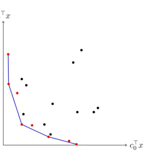
f1(x)
f2(x)
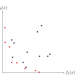
Figure 1.1: Projection of the feasible set X onto the span of the objectives f1(x) and f2(x). Pareto-frontier (red).
in quality, and maximizing a tank capacity contradicts the aim for a minimum weight. Criteria may though be totally unrelated, for example, when a solution has to comply with the requirements of engineering, logistics, economics and environment at the same time.
For this reason, it is not the original objective in multicriteria optimization to find one common optimal solution, which most likely does not exist. Instead a set of so-called non-dominated solutions is considered.
Definition 1.31. A feasible solution x ∈ X is said to (Pareto-) dominate a feasible solution y∈X, if, assuming minimization,
(1) fi(x)≤fi(y) for all i= 1, . . . , k and
(2) fj(x)< fj(y) for at least one j ∈ {1, . . . , k}.
Definition 1.32. A feasible solution x∈X is(Pareto-) efficient or (Pareto-) op-timal, if there does not exist another solution that dominates it. The corresponding vectorf(x) is called a non-dominated point.
The set of all Pareto-efficient solutions constitutes the so-called Pareto-frontier and by abuse of notation is often referred to as the set of non-dominated points in the image domain (see Figure 1.1). The concept of efficiency is in most cases related to the decision space X, while the concept of dominance refers to the criterion spacef(X). The name goes back to Vilfredo Pareto, who introduced and extensively used this concept in his contributions to the field of microeconomics [63].
1 2 0 n−2 n−1 n (1,0) (2,0) (0,1) (0,2) (2n−2,0) (2n−1,0) (0,2n−2) (0,2n−1) . . .
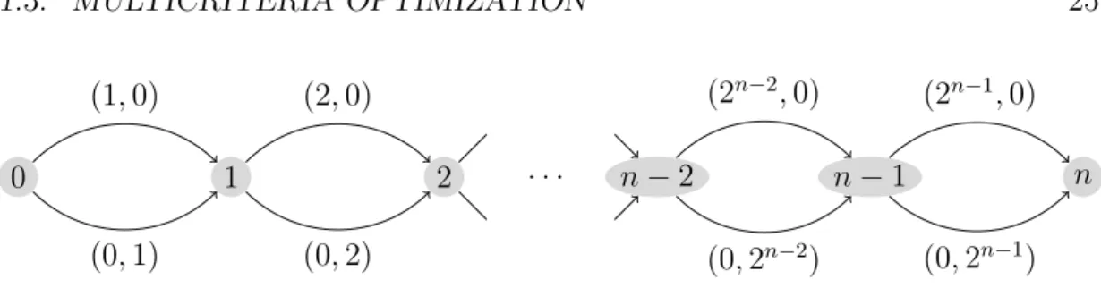
Figure 1.2: A Shortest Path-instance with an exponential number of efficient solutions.
If no additional subjective preference information is given, the Pareto-efficient solutions are considered equally good. Hereby, the biggest problem is that there might exist exponentially many efficient solutions:
Example 1.33. Consider the Shortest Path-problem on the graph in Figure 1.2. Here, all feasible solutions (all 0−n-paths) are Pareto-efficient: Sorting them in ascending order by the values of the first function, we get the set of non-dominated points in the image domain
{(0,2n−1),(1,2n−2),(2,2n−3), . . . ,(2n−3,2),(2n−2,1),(2n−1,0)},
which is of exponential size.
In this regard, a large variety of goals, philosophies and methods were developed in multicriteria optimization. Tosolve a multicriteria optimization problem can mean
• to find all Pareto-optimal solutions,
• to find a representative set of Pareto-optimal solutions, or
• to find onemost preferred solution due to some certain subjective preferences criteria.
In the last point we can distinguish betweenupfront anda posteriori preferences. The a posteriori methods are mostly based on estimations of a human decision maker, who can assess which solution is a good compromise in a given application. In the upfront methods, Problem (1.1) is often converted into a single-objective problem. A famous approach here is, for example, theweighted sum method [56]. An overview of fundamental concepts, methods and results on multicriteria opti-mization is given in [34].
Robust Optimization under
Ellipsoidal Uncertainty
Now we discuss the actual topic of this thesis, namely robust combinatorial optimization under ellipsoidal uncertainty, in a greater detail. To this aim we will in Section 2.1 motivate and demarcate the idea of robustness and give an overview to the existing approaches, with the focus on strict robustness, as it is the central paradigm in this thesis. In this context we introduce different uncertainty sets and outline the corresponding complexity results.
As ellipsoidal uncertainty is our basic topic, we go into more detail and dedicate the Sections 2.2 to 2.4 to this uncertainty set. There we describe in detail the existing solution approaches and summarize the complexity results known in the literature. We not only introduce basic definitions but also discuss and prove some fundamental statements, such that we can build on this prior knowledge in the following chapters.
2.1
Robust Optimization
An abstract optimization problem
min f(x)
s.t. x∈X, (2.1)
with the objective functionf and the feasible setX, becomes a real-world situation as soon as concrete data is given, for example, a specific network with the costs or duration of proceeding through every edge. But in fact, the data is hardly ever known precisely, but subject to uncertainty caused by various matters. It can have a social, ecological or financial character, like uncertainty about the exact soil conditions while planning new power lines and related costs. It can be caused
by future and unpredictable events, like political decisions or natural disasters with associated loss of capacities. Disposal over only inexact or estimated data or limited access to information, as well as a simple measuring errors, also may produce uncertainty.
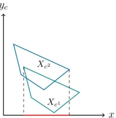
In the following we assume to be given an uncertain optimization problem of the form
min f(x, c) s.t. x∈Xc,
(2.2) where the objective function and the feasible set now in some way depend on a random variable c. For a fixed cProblem (2.2) becomes a certain Problem of the form (2.1), which we sometimes refer to as the nominal or deterministic problem. In order to solve an optimization problem, we aim to find a feasible solution having the best objective value. Now with uncertain data, feasibility and/or optimality of a solution might be affected. Sometimes even small perturbations may lead to a complete uselessness of a chosen solution, while the decision-making process does not allow any changes of the adopted solution after the data reveals itself. What is the chosen solution worth, if its optimality or even feasibility are not guaranteed any more? The concept of optimality or even solution must be redefined when dealing with uncertainty. Uncertainty must be taken into account already in the problem definition.
The concept of scenario is a common and natural way to structure uncertainty. Usually it is at least possible to overview all the relevant scenarios, how the data may behave, and to put these together in a so-called uncertainty set U. While redefining feasibility and optimality, it makes sense to ask for feasibility in every possible scenario and for certainguarantee of quality. This is a common thought in all existing robustness criteria. Many such criteria were proposed in a short time.
In the following we describe different approaches to define the so-called robust counterpart of Problem (2.2) and summarize the most important forms of U.
2.1.1
Strict Robustness
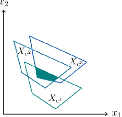
The strict robustness was first mentioned by Soyster [70] and was extensively studied since then [10, 35, 13, 15]. The initial idea to call a solution robust against uncertainty is to require its feasibility and possibly good quality in every possible scenario (see Figure 2.1).
Such a perfect solution though may hardly exist. The general way out in robust optimization is to accept some quality loss against certain immunity to parameter changes. The idea of strict robustness is to consider the worst-case scenario, to be sure that the value of the solution would not get any worse in any case. But the worst-case scenario might vary from solution to solution, such that it might not be
x2
x1
Xc1
Xc2
Xc3
Figure 2.1: Strict Robustness: The feasible set of a strictly robust problem is the intersection of the feasible sets in every scenario.
enough to consider one bad scenario. Strict robustness considers for every solution its value in its worst-case scenario and compares solutions regarding these values, i.e. it solves the problem
min max
c∈U f(x, c)
s.t. x∈Xc for all c∈ U.
(2.3) This criterion is occasionally called min-max-robustness or absolute robustness. We minimize the maximum value a solution can reach among all possible scenarios from the uncertainty setU. Problem (2.3) defines the so-called robust counterpart of the uncertain Problem (2.2) in the case of strict robustness.
Here, the difference to stochastic programming, which is another approach to deal with data uncertainty, has to be emphasized: We do not consider or estimate any probability distributions of the scenarios to get a good solution on average, but we want to be free of risk in every reasonable scenario, no matter how likely or unlikely it is to occur.
It must be said that this great pessimism also can be seen as a limit of this approach. Sometimes really improbable bad cases are strongly overestimated, such that the provided solution is very conservative and can be far away from the optimum in the realized scenario. This trade-off between risk-aversion and optimality is often referred to asprice of robustness [14].
A related and less conservative approach to define an optimal solution under uncertainty is min-max-regret [2]. It aims to minimize theregret one might feel when the data reveals itself and the chosen solution cannot be changed any more, i.e. the difference between the value of the optimal solution in the realized scenario and the value of the chosen solution. The corresponding robust formulation is
min max c∈U f(x, c)−f(x ∗ c, c) s.t. x∈Xc for all c∈ U, (2.4)
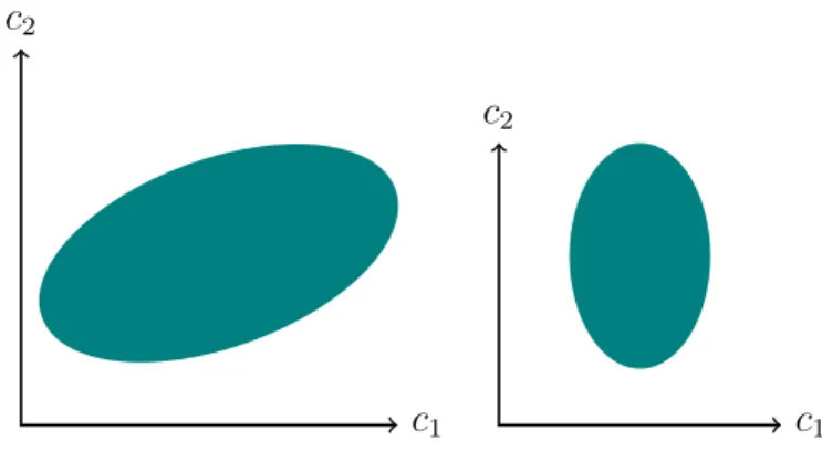
c2
c1 (a) Interval uncertainty
c2
c1 (b) discrete scenario case
c2 c1 (c) Γ-uncertainty c2 c1 (d) polytopic uncertainty c2 c1 (e) ellipsoidal uncertainty Figure 2.2: Uncertainty sets. wherex∗c denotes the optimal solution in scenario c.
In general, Models (2.3) and (2.4) yield different solutions. The usage of one or another criterion depends on their appropriateness in a given application. The min-max-regret criterion is preferred in situations, where the importance of a comparison between the performances of different actions or actions of the opponent actors is crucial. This can be the case, for example, in the investment management, where the opportunity costs play a major role.
2.1.2
Uncertainty Sets
The complexity of and approaches to the robust counterparts (2.3) differ funda-mentally depending on the definition of the uncertainty setU. Clearly, in different situations the possible scenarios may constitute differently shaped sets. But the main criterion to consider different forms of U is the tractability of the resulting counterparts.
2.1.2.1 Boxes
One natural way to describe the set of possible scenarios is to define a lower and an upper bound on every uncertain coefficient, assuming that the costs may vary within the corresponding intervals. This leads to a box form of the uncertainty set (see Figure 2.2(a)) and the uncertainty type is called interval uncertainty [2].
From the practical point of view this case is rather attractive but theoretically uninteresting. The coefficients are completely unrelated to each other and the worst case of every solution is the same, namely the scenario with all coefficients being on their upper bounds. In this case the robust counterpart preserves the complexity of the certain Problem (2.1):
Theorem 2.1. [2] The robust counterpart of (2.2) with interval uncertainty is solved by solving the nominal problem (2.1) with the worst-case scenario.
On the other hand, the optimal solution is over-conservative, given the fact that the case with all coefficients on their upper bounds is very unlikely to happen, which makes the user accept an unnecessarily bad value. These two facts make it worth to consider different forms of uncertainty.
2.1.2.2 Finite Sets
In some situations the set of possible scenarios is explicitly given. Such situations are called discrete-scenario case (see Figure 2.2(b)). Here, the challenge is to reduce the cardinality ofU as far as possible, due to the following.
Theorem 2.2. [50] In the discrete scenario case the problem min max
c∈U c >
x
s.t. x∈X (2.5)
is N P-hard, even for |U |= 2 and some X where linear optimization is easy. Here and in further considerations we assume a linear objective function of the nominal problem, i.e.f(x, c) = c>x.
This result originates from [50] for the Shortest Path-problem, the Minimum Spanning Tree-problem, Minimum Cost Assignment and Resource Scheduling and was shown in [6] for the unconstrained caseX ={0,1}n.
Nevertheless, for a constant number of scenarios many combinatorial problems can be solved in pseudo-polynomial time. But if the number of scenarios is part of the input, these problems become strongly N P-hard (see [2] for an overview).
2.1.2.3 Trimmed Boxes
Another uncertainty set is proposed in [13] and allows to adjust the level of conservatism in contrast to the interval uncertainty. The authors suggest that it is very unlikely that all coefficients differ from the expected scenario at the
same time and restrict the number of changing coefficients to at most Γ≥0. The uncertainty set can be written as
U ={c∈[l1, u1]× · · · ×[ln, un]|#{I ⊆ {1, . . . n} | |un−c0n|>0} ≤Γ},
where c0 denotes the vector of the coefficients in the expected scenario, and is called Γ-uncertainty.
The parameter Γ allows to control the value of conservatism, while the correspond-ing robust counterpart remains computationally tractable.
Theorem 2.3. [13] The robust counterpart (2.5) with Γ-uncertainty is reduced to solving n+ 1 corresponding nominal problems (2.1) ifn is the number of variables. Another variant of Γ-uncertainty is to restrict thetotal deviation from the expected scenario [18], i.e. U = ( c∈[l1, u1]× · · · ×[ln, un]| n X i=1 |ci− li+ui 2 | ≤Γ ) ,
(see Figure 2.2(c)). Also here Problem (2.5) is reduced to solving n+ 1 nominal problems, which can be shown in analogy to [13].
2.1.2.4 Polytopes
Interval and Γ-uncertainty are special cases of polytopic uncertainty. Here, the uncertainty set is a general polytope:
U ={c∈Rn|T c≤s},
with T ∈Rr×n and s∈Rr [18] (see Figure 2.2(d)).
Since U = conv(v1, . . . , vk) for some suitable k due to the Weyl-Minkowski
Theo-rem [58], the following result applies.
Theorem 2.4. The robust Problem (2.5) with polytopic uncertainty is at least as hard as with discrete uncertainty and a fixed number of scenarios, even for some
X where linear optimization is easy.
Since for a fixed finite number k of points their convex hull, which is a polytope, can be constructed in linear time, the discrete scenario case for a fixed number of scenarios, which can be hard due to Theorem 2.2, reduces to Problem (2.5) with polytopic uncertainty.
We hold down that the polytopic uncertainty is in general hard to treat, while some easy special cases, such as interval and Γ-uncertainty, exist.
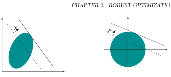
2.1.2.5 Ellipsoids
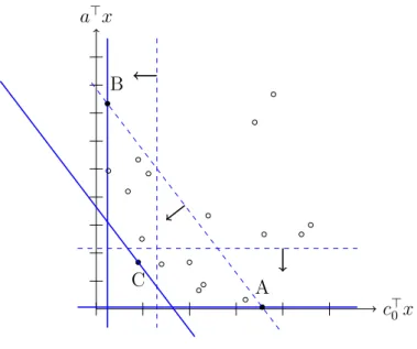
In the focus of this thesis isellipsoidal uncertainty, whereU is given by an ellipsoid inRn: U = c∈Rn| q (c−c0) > A−1(c−c 0)≤r ,
with c0 ∈Rn, r >0 andA ∈ S++n (see Figure 2.2(e)). HereS++n denotes the set of
all positive definite matrices of order n.
Here the costs are assumed to be caused by some normal distribution with mean
c0 and a covariance matrix A, which relates to many applications (see Section 2.2 for motivation of this notation). This form of uncertainty is less conservative than interval uncertainty since the very unlikely extreme points ofU, where the worst case is taken in the interval case, is explicitly excluded here. Moreover, it allows to model correlations between the coefficients, both positive and negative. Finally, it is practically and theoretically interesting, as it incorporates both tractable and intractable special cases, as well as some still not specified cases.
2.1.3
Different Approaches
Strict robustness is very conservative and in many cases intractable. Also, in many applications different conditions apply, such that in the last two decades alternative robustness approaches have been developed. These define different criteria of robust optimality. Here, we shortly mention some of these approaches.
2.1.3.1 Recoverable Robustness
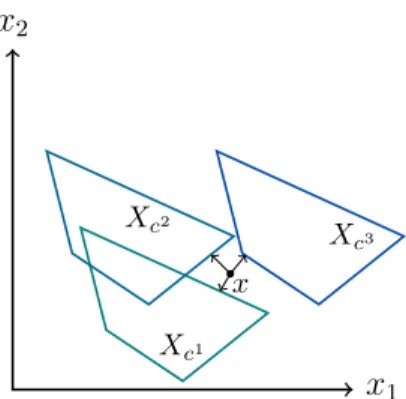
The concept of recoverable robustness was formalized in [53]. The idea is to find a solution which may become infeasible or bad when the data becomes certain, but which can then berecovered to a feasible or a better solution by means of one of the given recovery algorithms (see Figure 2.3).
Recoverable robustness hence distinguishes two phases: A planning phase and arecovery phase. A setA of admissible recovery algorithms is given beforehand and specifies the recovery possibilities. In the planning phase a solutionx and an algorithmA ∈ A are determined. A specifies how x can be recovered for every scenario. In the recovery phase (when a scenario is realized), the algorithm A is used to turn the solution x into a feasible solution for the realized scenario. The recovery robust problem can be formulated as
min f(x)
s.t. A(x, c)∈Xc for all c∈ U
(x, A)∈X× A,
x2 x1 Xc1 Xc2 Xc3 x
Figure 2.3: Recoverable robustness.
whereXc denotes the set of feasible solutions in the scenario c.
Note that the solution of Problem (2.6) is a tupel (x, A). If no recovery is possible for any solution x by means of the given set of algorithms, Problem (2.6) has value∞.
Obviously, the set of recovery algorithms should be limited due to some reasonable criteria, which mostly concern two main aspects:
• the recovered solution must not be too far from the recoverable solution x
with respect to a certain measure of distance;
• the computational effort of the algorithmAto turn the solutionxto a feasible solution should be restricted, preferably in terms of the computational effort to compute the solution x in the planning phase.
If A consists of exactly one algorithm A withA(x, c) =x for all c∈ U, then we are in the case of strict robustness.
Since its first formalization, recoverable robustness has been applied in the context of railways, shunting, timetabling and delay management and many other fields [26, 27]. Clearly, it strongly depends on the underlying problem and on the set A whether Problem (2.6) is tractable or not.
2.1.3.2 Adjustable or Two-Stage Robustness
In adjustable or two-stage-robustness [11] certain variables are allowed to be determined after the realization of a scenario. The set of variables is decomposed into
• the here-and-now variables x ∈ Rn1, which have to be determined in the first stage, i.e. before the realization and
yc
x
Xc1
Xc2
Figure 2.4: Adjustable robustness.
• the wait-and-see variables yc ∈ Rn2, which have to be determined in the second stage, i.e. after the realization of a scenario.
The goal is to find anadjustable solution x∈Rn1, i.e. such that for every c∈ U there exists a yc ∈ Rn2 such that (x, yc) is feasible for c. The adjustable robust
problem is
min
x∈Rn1 maxc∈U min f(x, yc, c) s.t. (x, yc)∈Xc
yc∈Rn2
(2.7)