Neighbouring Link Travel Time Inference Method Using Artificial Neural Network

Neighbouring Link Travel Time Inference Method

Using Artificial Neural Network

Luong H. Vu

, Benjamin N. Passow, Daniel Paluszczyszyn, Lipika Deka and Eric Goodyer

De Montfort University, Leicester, United Kingdom ∗_{Email: [email protected]}

Abstract—This paper presents a method for modelling relation-ship between road segments using feed forward back-propagation neural networks. Unlike most previous papers that focus on travel time estimation of a road based on its traffic information, we proposed the Neighbouring Link Inference Method (NLIM) that can infer travel time of a road segment (link) from travel time its neighbouring segments. It is valuable for links which do not have recent traffic information. The proposed method learns the relationship between travel time of a link and traffic parameters of its nearby links based on sparse historical travel time data. A travel time data outlier detection based on Gaussian mixture model is also proposed in order to reduce the noise of data before they are applied to build NLIM. Results show that the proposed method is capable of estimating the travel time on all traffic link categories. 75% of models can produce travel time data with mean absolute percentage error less than 22%. The proposed method performs better on major than minor links. Performance of the proposed method always dominates performance of traditional methods such as statistic-based and linear least square estimate methods.

Keywords—travel time estimate; sparse historic data; artificial neural network; traffic model

I. INTRODUCTION

Travel delays due to traffic congestion cause a huge waste of money increased human stress and unsafe traffic situations. They also increase negative environmental and societal side effects [1]. According to [2] the United Kingdom is the worst country in Europe in terms of traffic congestion, and London is the most congested city in the continent (The estimated congestion cost drivers in the UK more than £30 billion in 2016 alone). Congestion can be defined as the traffic demand exceeding the roadway capacity. In urban areas, transportation infrastructure development is constrained by land and financial resources [3]. In order to deal with growth, advanced dynamic traffic management systems are needed to manage existing transportation systems efficiently. Such systems require highly efficient and dynamic models. Real time traffic information updated from traffic models and these models can be used to optimise signal control settings [4] and to help commuters avoid traffic congestions. A valuable and objective type of traffic information is the travel time [1].

Historical travel time and other related parameters can be measured and collected typically by using stationary observers or moving observers. Stationary observers include loop de-tectors and video surveillance, which provide flow and speed

estimation at regular and frequent intervals. Moving observers, consisting of floating cars or probe cars, provide information which can be used to extract travel time data in road segments where the probe cars go through [5]. Travel time data source directly impacts on the property of travel time data. Stationary observers can produce travel time data at regular and frequent intervals for a particular highway or major road and they leave the traffic information in the rest (minor roads) of the network unknown [6]. In contrast, the moving observers can produce travel time at irregular and less frequent intervals. However, they can only cover a limited number of routes for a limited duration of time. Hence, for a particular road segment, there might not be any travel time data available [5], [7]. Thereby, travel time data are sparser for segments of non-major roads. Travel times are different in different road categories [8]. Travel time data on motorways regularly show relatively low variability, especially in congested conditions. They mainly depend on geometrical characteristics of motorways, such as the number of ramps weaving sections per unit road length [9]. In contrast, urban travel times can reveal very high variability because of traffic light signal cycles and queue delay affect travel times to a large extent. Pedestrian and cyclist disturbance, transit priority and parking often affect travel time [1], [5]. Therefore, it is difficult for a model or an algorithm to estimate accurately near real-time travel time in urban areas.

We propose the Neighbouring Link Inference Method (NLIM) to deal with sparse travel time data in a large scale urban traffic network. NLIM learns the relationship between travel time of a road segment (link) and traffic parameters (travel time, vehicle class, time of day, the day of a week) of its nearby links using feed forward back propagation neural networks (FF-BP-ANNs). Thereafter, the NLIM model is used to estimate near real-time travel time data for links which do not have recent observed travel time data.

A travel time data outlier detection based on Gaussian mixture model (GMM) is also used in order to reduce noises of data before they are applied to build the NLIM models. To assess the performances of NLIM, it is compared to performances of expectation and linear least square estimate (LLSE) methods. Results show that the NLIM outperforms the expectation and LLSE method.

II. RELATEDWORKS

There are numerous methods to model travel time. Linear regression models [10], [11] are employed to learn the rela-tionships between future travel time and recent travel time in time series. The models were trained and tested using motorway travel time. Various traffic patterns during different days in a week were considered. They are simple, stable, and computationally efficient. The Bayesian inference-based dynamic model described in [12] provides distribution of predicted travel times and their confidence intervals. Math-ematical model proposed in [13] incorporate data collected in a period of time to provide accurate estimates for the mean of travel times and traffic condition on the traffic links. The probabilistic model introduces in [14] merges the spatial and temporal travel time information to obtain accurate short-term travel time prediction for motorway corridors under different traffic conditions. Statistics model in [6] is used for urban road network travel time estimation using vehicle trajectories obtained from low-frequency GPS probes, where the vehicles typically cover multiple network links between reports. GMM proposed in [15] represents travel time distributions on arterial roads with signalised intersections. The proposed model is applicable to travel time data from both fixed and mobile sensors. Support vector machine technique is in [7] employed and used information from nearby links to predict travel time of a link, called geospatial inference. The model, which is based on the support vector machine, relies on time series floating car data to predict future travel time data of a selected link from its specific nearby links. Artificial neural network (ANN) in [16], [17] use historical travel time and actual travel time to predict long distance travel time. ANN has also been employed in [18] to an estimation of complete link travel times based on partial link travel times or route travel times.

Up to now, most of these models require the information of historical travel times which are complete link travel times, route travel times or partial link travel times with regular and very high frequent intervals to estimate or predict travel times. As a result, most research up to date is based on time series travel data.

To optimise signal control setting as well as to help com-muters make a decision for route selection and planning, travel times of links in a traffic network should be provided. Installing stationary observers on a network is a quite costly solution. An alternative cost-effective solution is utilisation of travel time data produced by moving observers such as vehicles equipped with tracking devices (e.g. GNSS). Unfor-tunately, travel time data from vehicles equipped with tracking devices are sparse; only a limited number of roads are covered in a particular time interval.

The main characteristics of our work that differentiate it from related works are

• the use of sparse historical travel time data,

• the ability of estimating the travel time from nearby link travel time data,

• and the ability to apply the model in a large scale traffic network.

III. NEIGHBOURINGINFERENCEMETHOD

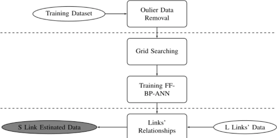
The Neighbouring Link Inference method has three key processes presented in Figure 1: data outlier removal, learning relationship between links and estimating travel time data. A. Outlier Travel Time Data Detection

Theoretically, collected travel time is real travel time of a vehicle travelled over a traffic road. However, travel time data might have a number of high-value data points because frequent stopping or starting would report much slower travel time than that actually prevails on the road. The data we have, shows heavy right skewed distributions and the means are typically five times greater than the medians.

In statistics, an outlier is an observation point that is distant from other observations. On overall, statistical characteristics are influenced by outliers and they may lead to erroneous conclusions. Therefore detecting outliers is necessary before utilising data to obtain a reasonable solution to a problem [19]. Several approaches have been used to detect and remove outliers; these range from statistics, to ANNs and fuzzy algorithms [19]–[21].

Study of [15] shows that GMM is able to produce high ac-curacy rate of vehicle stop/non-stop movement classification. Therefore GMM can be utilised to detect outlier in sparse travel time data. GMM is a probabilistic model based on the Gaussian distribution. The mixture describes the probability distribution of an observation x in the overall population. GMM is defined as: N(x|µ, σ) = 1 (2π)D/2 1 |σ|1/2exp{− 1 2(x−µ) T_σ−1_(x −µ)} (1) p(x) =σ_kK₌₁πkN(x|µk, σk) (2)

Where K is the number of Gaussian components, µ1...µk

are the means of components, µ is vector composed of all the individualµ1...µk,σ1...σk are the variances of each

com-ponents, σ is vector composed of all the individual σ1...σk,

D is the dimension of the observation vector x. π1...πk are

mixture weights,N(x|µk, σk)is a probability density function

of Gaussian distribution and p(x) is posterior distribution of x.

GMM is an unsupervised clustering method which ac-commodates clusters that have different sizes and correlation structures within them. Every cluster is described by the mean vectorµ and the covariance matrixσ. The cluster member is assigned based on the probability that has been generated using itsµ andσ.This probability is computed using formula (3):

p(x|π, µ, σ) =πp(x) (3) In this work, a travel time outlier detection based on GMM is proposed for filtering outliers of travel time data. Structure and size of a cluster are utilised to determine/detect outlier data in our proposed algorithm. Threshold parameters are defined to distinguish normal data from outlier data.

We separately apply travel time data outlier for data of each vehicle category because different vehicle classes might have

Oulier Data Removal Training Dataset Grid Searching Training FF-BP-ANN Links’

Relationships L Links’ Data S Link Estinated Data

Fig. 1. Overview of Neighbouring Link Inference Method

distinguishable characteristics and behaviours, therefore, they might produce different travel time distributions. Travel time data set of a link was split into 9 subsets that belong to 9 vehicle classes.

The steps of travel time data outlier detection based on GMM are described in Algorithm 1.

Algorithm 1 Outlier Detection

1: function OUTLIERDETECTION(τ, , K) . Whereis a predefined threshold,τ is travel time data set

2: Apply GMM forτ to getµi,σi andπi (i=1,2,...,K).

WherePK

j=iπi = 1 3: fori= 1toK do 4: ifπi≤ then

5: Remove data of Component i

6: end if 7: end for 8: end function

B. Learning Relationship Between Links

In this section, we propose a method to model the rela-tionship between travel time of a link and traffic parameters (travel time, vehicle class, time of day, the day of a week) of its nearby links based on feed forward back propagation neural network (FF-BP-ANN). Feed Forward ANN with Back Propagation algorithm has been widely used in solving various classification, estimation and forecasting problems [6], [16], [17], [21].

1) Grid Searching: There are several parameters of ANN which are needed to be adjusted before training. Choosing training algorithm is one of the most important decisions. There is no training algorithm that is the best for every problem. Training algorithms have several different parameters such as steepness, learning rate, momentum which can be set. For Incremental, Batch and Quick-prop training algorithm, the most important parameter is the learning rate, but un-fortunately, this is also a parameter which is hard to find a reasonable default value for them. It is also worth noting that

the activation function has a profound effect on the optimal learning rate [22].

Algorithm 2 Grid Searching

1: function GRIDSEARCHING(Dp) .WhereDp is training

data set

2: Θ ={L, H1, H2, ..., HL} . Where N is number of

training samples that will be used for grid searching, L is number of hidden layers, Hi is number of hidden nodes

inith hidden layer

3: ∆ ={a, m, s, l} . Whereais an activation function, m is momentum,sis steepness and l is learning rate

4: DN ←Randomly select N samples onDp 5: Set training algorithm is Incremental

6: Edesired←1e−9 .WhereEdesired is desired error 7: Ebest← ∞

8: for eachδi∈∆ andθj∈Θdo

9: Train M{δ, θ} on DN using 3-folds

cross-validation

10: Compute MSE of outputs based on Equation 4

11: if errorbest< M SE then

12: errorbest←M SE 13: δbest←δi 14: θbest←θj 15: end if 16: end for 17: end function

When creating a network it is necessary to define how many layers, neurons and connections that an ANN should have. If the network is too large, the ANN will meet difficulties in learning and the results tend to over-fit resulting in poor generalisation. If the network becomes too small, it will not be able to represent the rules needed to learn the problem and as a result, it will never gain a sufficiently low error rate.

The number of hidden layers is also important. ANNs with one or two hidden layers are enough for a simple problem, but more hidden layers might be needed with complicated problems. The correct number of hidden layers and number of hidden neurons for a particular application is important. For

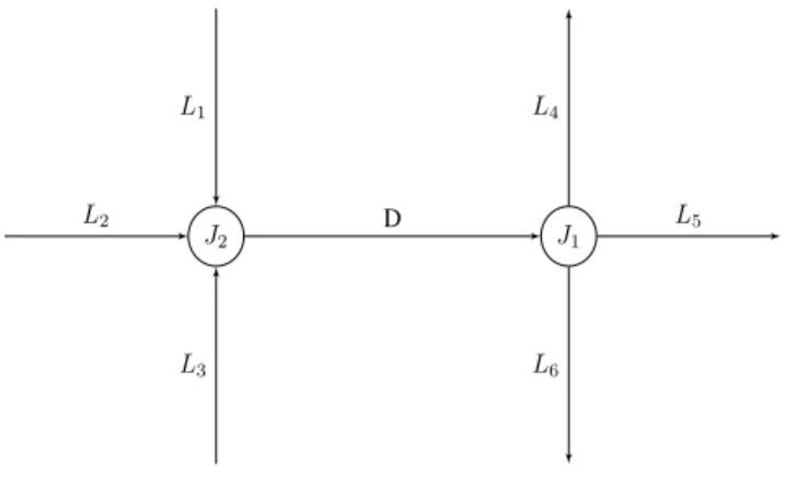
J1 J2 D L1 L3 L2 L4 L6 L5

Fig. 2. A Link Layout

example, it is seen that in [21], number of hidden layers and number of hidden nodes heavily affects the performance of FF-BP-ANN that was trained on the original data set as well as on the data that were applied to an adaptive filter.

If too much training is applied to a set of data, the ANN would over-fit and thereby loose generalisation. Testing with unseen data can be done while doing training to see how much training is required to make sure ANNs perform well without over-fitting. Therefore, 3-folds cross-validation is utilised in a searching procedure. The incremental training algorithm is also chosen because it gives more control for stop criteria of the training loop.

A number of data samples in each model is varying from hundreds to thousands. It is possible to conduct the grid searching on the whole data set. However, it is time-consuming if the number of data samples is large. Especially when a large number of models needed to be processed, it would be extremely time-consuming. Therefore reducing time con-sumptions for each model testing is valuable. Hence, only 1000 data samples in each model have randomly chosen if the number of complete data samples is greater than 1000. The grid searching is then conducted on them, and the found parameters are applied to ANN for training on the complete data set subsequently.

The mean square error (MSE) is used to assess the perfor-mance of an ANN with structural differences. MSE is defined as below: M SE= 1 n n X i=1 ( ¯ti−ti)2 (4)

Wheret¯i is the estimated travel time,ti is the observed travel

time and nis the number of observations.

In this work, a grid searching for a FF-BP-ANN structure and its parameters is applied because grid searching can offer parallel computation to reduce overall processing time. Details of grid searching for parameters of FF-BP-ANN is shown in Algorithm 2.

2) Training FF-BP-ANN: In this work, a link layout is defined as a combination of a designated link (D) and its neighbouring links (L). A typical link layout is shown in Figure 2. The arrows in the link layout are the direction of

vehicles movement in a link. A full neighbouring model is defined as a model that contains all links in a link layout. For example, in Figure 2, the full neighbouring model is

{D, Lj}, j= 1,2, ...,6.

If there was enough number of data samples on each link in a link layout, only the complete model would be usually used because it presents completely relationship of links in a link layout. Unfortunately, every link in a link layout has different data sparse rate and some of them have an insufficient number of the data sample. Consequently, the larger number of neighbouring links is combined in a model, the lower number data samples model it might have. Hence, a set of models for a designated link, which are made from all possible combination of the designated link and its neighbouring links, are considered. Every model, which have larger than 25 data samples, are carefully trained and tested.

Algorithm 3 Neighbouring Links Inference Method

1: function NLIM(Dp) .WhereDp is training data set

2: maxIter←10000

3: Edesired←1e−9

4: increasedCon←3

5: Set training algorithm is RPROP .The RPROP training algorithm is adaptive, and does therefore not use the learning rate

6: forp=1 toξ do

7: Vp←Select 40% ofDp 8: Dp←Dp-Vp

9: (δbest, θbest)←GRIDSEARCHING(Dp)

10: M SE←0

11: inc←0

12: iter←0 13: M SEbest←∞

14: while M SE ≤ Edesired and inc ≤

increasedCon anditer≤maxIter do 15: TrainMp(δbest, θbest)onDp

16: Compute MSE ofMp onVp 17: iter←iter+ 1 18: ifM SE > M SEbest then 19: inc←inc+ 1 20: else 21: inc←0 22: M SEbest←M SE 23: end if 24: end while 25: SaveMp 26: ComputeM AP Ep on Vp, saveM AP Ep 27: end for 28: end function Assume theith_{link (L}

i) of N links in a traffic network has

ni neighbouring links Li,j, j=1,2,..,ni. Number of possible

models for N links (ξ) is compute with formula (5)(6):

ξ= N X i=1 ni X k=1 ni_C k (5)

ni_C

k =

ni(ni−1)...(ni−k−1)

k(k−1)(k−2)...1 ,(k≤ni) (6) Data of a model has following features: day of a week, time of day, vehicle class, travel time data of designated link and travel time data of selected neighbouring links. Each model is trained using Neighbouring Link Inference Method (NLIM) presented in Algorithm 3.

Mean absolute percentage error (MAPE) is used to compare the performance of an ANN trained by NLIM. MAPE is defined below: M AP E=100 n n X i=1 |ti−tˆi ti | (7)

Whereti is the observed travel time,tˆi is the estimated travel

time and nis the number of observations. IV. EXPERIMENTALRESULTS

A. Experimental Data

The proposed methods have been evaluated with use of travel time data collected from September 2009 to February 2012 in Leicestershire, UK. The dataset comprise travel times for 3200 traffic links. The raw data collected from GNSS locations contain reconstructed link travel times at 15 min intervals. Thereby, a day starting from 00h00 to 23h59, was divided equally into 96 time slots.

TABLE I

DATA SPARSE RATES(%)ONMOTORWAY, TRUNK, PRIMARY, A, B, MINOR LINK TYPES OBSERVED ON HISTORICAL DATA SETS.

Urban Mo- tor-way Trunk Pri-mary A B Mi-nor Lower whisker 93.1 98.7 100 100 100 100 Lower quartile 25% 54.9 81.5 85.0 85.9 90.5 97.7 Median 19.5 74.6 77.6 81.3 87.1 95.5 Upper quartile 75% 10.5 40.2 70.7 76.8 83.7 92.9 Upper whisker 0.0 20.0 36.9 0.0 39.9 68.6

Data sparse rates of link types are shown in Table I. Data sparse rate was defined as density of the travel time samples available in data set individual link. Furthermore, if each time slot from September 2009 to February 2012 has at least one data sample than data sparse rate of the link is 0%. If there is sixty percent of time slots having at least one data sample than the sparse data rate of the link is 40%.

The statistics in Table I indicate that data are more sparse on the urban traffic links than on the motorway links. The lower quartile, the median and the upper quartile of data sparse rate on motorway links are 54.9%, 19.5% and 10.5% respectively. Their values are significantly greater on the urban links. B. Experimental Setting

Outliers of data set on 3200 traffic links are detected using the outlier method proposed in the previous section. We assume that travel time data of every vehicle class on the 3200

traffic links follow Gaussian mixture model with 3 components (k=3). Any Gaussian component that has proportion less than 10% ( = 0.1) is considered as a set of travel time outliers. was set to 10% because of heavy right skew distribution of travel time on traffic links that were observed from the data set. Input features for training and testing the proposed method in a link layout are sparse historical travel time of neighbouring links, time of day(time slot), vehicle class and day of a week. Day of a week is inferred from date of a year. Output feature is historical travel time corresponding to the input features of a designated link.

3200 links produce 3200 link layouts. There are 12566 travel time models in total. The models from all link layouts are carefully trained, verified and tested to make sure relation-ships between links on each link layout are correctly learnt and these relationships are stable over the experiments. The performances of models are evaluated by MAPE on unseen data.

To assess performances of NLIM, historical travel time data sets are also fitted to traditional methods: Linear least square estimate (LLSE) and Statistic-based method. Thereafter, per-formances of NLIM will be compared to perper-formances of LLSE and Statistic-based models.

The LLSE learns the linear relationship between travel times of two links model every pair of links in a link layout for

0 10 20 30 40 50 60 70 0 5 10 15 20

Mean Absolute Percentage Error (MAPE) [%]

Density

of

Models[%]

Statistic-based LLSE NLIM

Fig. 3. Relationship between density of models and their MAPE [%] achieved by Statistic-base, Linear Least Square Estimate(LLSE) and Neighbouring Link Inference Method (NLIM) on unseen data.

TABLE II

PERFORMANCE OFSTATISTIC-BASED, LLSE, NLIMOF ALL LINK CLASSES EVALUATED BYMAPEON UNSEEN DATA.

Statistic-based LLSE NLIM

Lower whisker 13.17 11.00 3.37 Lower quartile 25% 40.56 13.48 10.38

Median 41.27 17.64 13.90

Upper quartile 75% 57.76 25.75 21.87 Upper whisker 100.06 640.29 49.90

Statistic-based LLSE NLIM 0 10 20 30 MAPE [%]

(a) Motorway Links

Statistic-based LLSE NLIM

0 20 40 60 MAPE [%] (b) Trunk Links

Statistic-based LLSE NLIM

0 20 40 60 80 MAPE [%] (c) Primary Links

Statistic-based LLSE NLIM

0 50 100 150 MAPE [%] (d) A Links

Statistic-based LLSE NLIM

0 50 100 150 MAPE [%] (e) B Links

Statistic-based LLSE NLIM

0 50 100 150 200 MAPE [%] (f) Minor Links

Fig. 4. Relationship between density of the best statistic-based, LLSE and NLIM models of Motorway (a), Trunk (b), Primary (c), A (d), B (e) and Minor (f) links and their MAPEs [%] achieved on unseen data. Sub-figures are in different scales.

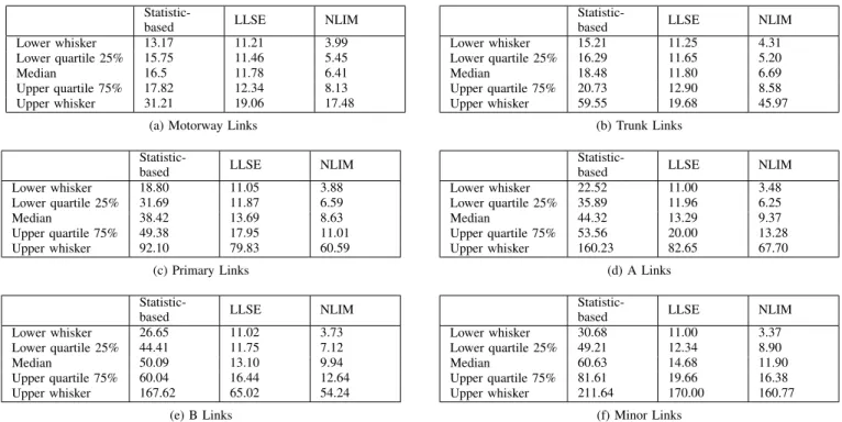
TABLE III

PERFORMANCE OF STATISTIC-BASED, LLSE, NLIMOFMOTORWAY(A), TRUNK(B), PRIMARY(C), A (D), B (E)ANDMINOR(F)LINKS EVALUATED BY MAPEON UNSEEN DATA.

Statistic-based LLSE NLIM

Lower whisker 13.17 11.21 3.99 Lower quartile 25% 15.75 11.46 5.45

Median 16.5 11.78 6.41

Upper quartile 75% 17.82 12.34 8.13 Upper whisker 31.21 19.06 17.48

(a) Motorway Links

Statistic-based LLSE NLIM

Lower whisker 15.21 11.25 4.31 Lower quartile 25% 16.29 11.65 5.20 Median 18.48 11.80 6.69 Upper quartile 75% 20.73 12.90 8.58 Upper whisker 59.55 19.68 45.97 (b) Trunk Links

Statistic-based LLSE NLIM

Lower whisker 18.80 11.05 3.88 Lower quartile 25% 31.69 11.87 6.59 Median 38.42 13.69 8.63 Upper quartile 75% 49.38 17.95 11.01 Upper whisker 92.10 79.83 60.59 (c) Primary Links

Statistic-based LLSE NLIM

Lower whisker 22.52 11.00 3.48 Lower quartile 25% 35.89 11.96 6.25 Median 44.32 13.29 9.37 Upper quartile 75% 53.56 20.00 13.28 Upper whisker 160.23 82.65 67.70 (d) A Links

Statistic-based LLSE NLIM

Lower whisker 26.65 11.02 3.73 Lower quartile 25% 44.41 11.75 7.12 Median 50.09 13.10 9.94 Upper quartile 75% 60.04 16.44 12.64 Upper whisker 167.62 65.02 54.24 (e) B Links

Statistic-based LLSE NLIM

Lower whisker 30.68 11.00 3.37 Lower quartile 25% 49.21 12.34 8.90 Median 60.63 14.68 11.90 Upper quartile 75% 81.61 19.66 16.38 Upper whisker 211.64 170.00 160.77 (f) Minor Links

particular vehicle class, time slot and day of a week. We assume that each link’s travel time has Gaussian probability density function (PDF). They are dependent on vehicle class, time slot and day of a week. Expected travel time value of a traffic link for a vehicle class on a time slot of a week day is the mean of the corresponding Gaussian distribution. From now on, this method is named statistic-based method. Performances of the LLSE and the Statistic-based method are also evaluated on unseen data.

C. Results

The proposed method is compared against statistic-based and linear least square estimate model. Figure 3 illustrates the relationship between density of models and their MAPE achieved by Statistic-based, Linear Least Square Estimate and Neighbouring Link Inference Method on unseen data. It can be seen that the introduced NLIM is capable of estimating travel times for a designated link using traffic parameters of its neighbouring links on all traffic link types.

Table II shows the statistical parameters of Statistic-based, LLSE and NLIM models tested on all link categories using unseen data. It can be seen that the upper and lower quartile of NLIM are 21.87% and 10.38% while those for LLSE are 25.75% and 13.38%. The percentage of E models that have MAPE less than or equal 20% is significant low which is less than 25%.

Next, the performance of the methods was evaluated with respect to a specific link category [8]. A designated link is modelled by multiple NLIMs. The performances of NLIM,

LLSE and Statistic-based model on a designated link are compared based on the performance of the best NLIM, the best NLIM and the best Statistic-based models in term of MAPE. Figure 4 present the relationship between density of the best NLIM, the best LLSE and Statistic-based models of Motorway, Trunk, Primary, A, B and Minor link category, and their MAPE achieved on unseen data respectively. The NLIM, LLSE and Statistic-based models perform better on major links than minor links. However, NLIM always dominates the others.

Their performance might be impacted by high data spare rate and high variability of urban travel time which is heavily affected by traffic light cycles, queuing delay, the pedestrian and cyclist disturbance, transit priority and loading. Further-more, the historical data collected on urban traffic network are contaminated with noise. As it can be seen in Table I, the data used in this research have a very high data sparse rate for the urban traffic links. Majority of links in the considered urban traffic network have data sparse rates greater than 70%. Especially on minor links, for which the data sparse rates are greater than 90%. This consequently makes the urban traffic links more difficult to model compared to the motorway links. From the Figure 4 and Table III, it can be seen that NLIM significantly outperforms all tested methods for all link types. The MAPEs of the best NLIMs models are significantly smaller. It might suggest that NLIM would be able perform well even in the case when data exhibit a high data sparse rate and is contaminated with a noise.

V. CONCLUSION

In this study, we have proposed a Neighbouring Link Inference Method (NLIM) that is able to learn the relationship between travel time of link and traffic parameters of its nearby links using FF-BP-ANNs. We also introduced a travel time outlier detection scheme based on GMM.

There are total 12566 travel time models from 3200 link layouts of Leicestershire urban traffic area are trained and tested on over 3 years of historical travel data using the NLIM. Roughly 10% of travel time data in a link are outliers. They are effectively detected by the proposed outlier method.

Every model having larger than 25 data samples are trained and tested. Results show that NLIM is capable of learning relationship between travel time data of a designated link and parameters of its neighbouring link on very complex sparse historical travel time data. 75% of NLIM models can produce travel time data on near-real time which have MAPE error less than 21.87%. 25% of NLIM models can estimate near-real time travel that have MAPE less than 10.38%. The best NLIM model has MPE at 3.37%.

NLIM was also evaluated with respect to a specific link category. The performance of NLIM method always dominates two traditional methods: Statistic-based and LLSE methods on all link types. The NLIM performs better on major links than minor links. It produces higher MAPE on the minor links than the major links. It might conclude that NLIM is able to precisely learn the relationship between links under the high data sparse rate and the high variability of urban traffic travel time.

In future work, we will focus on improving the performance of the Neighbouring Link Inference Method, especially in minor links, as the vast majority (70%) of links in the UK fall within the minor link category [8]. Thereafter, it would be used to build a large scale of an urban traffic model that can utilise knowledge of traffic links relationship to estimate the near real-time travel time of a link.

REFERENCES

[1] C. P. I. J. V. Hinsbergen, A. Hegyi, J. W. C. V. Lint, and H. J. V. Zuylen, “Bayesian neural networks for the prediction of stochastic travel times in urban networks,”IET Intelligent Transport Systems, vol. 5, no. 4, pp. 259–265, December 2011.

[2] G. Cookson and B. Pishue, “Inrix global traffic scorecard,” 2017. [3] N. Petrovska and A. Stevanovic, “Traffic congestion analysis

visualisa-tion tool,” inIntelligent Transportation Systems (ITSC), 2015 IEEE 18th International Conference on, Sept 2015, pp. 1489–1494.

[4] G. Abu-Lebdeh and A. K. Singh, “Modeling arterial travel time with limited traffic variables using conditional independence graphs &amp; state-space neural networks,”Procedia - Social and Behavioral Sciences, vol. 16, no. 0, pp. 207 – 217, 2011, 6th International Symposium on Highway Capacity and Quality of Service.

[5] X. Ma and H. N. Koutsopoulos, “A new online travel time estimation approach using distorted automatic vehicle identification data,” in2008 11th International IEEE Conference on Intelligent Transportation Sys-tems, Oct 2008, pp. 204–209.

[6] E. Jenelius and H. N. Koutsopoulos, “Travel time estimation for urban road networks using low frequency probe vehicle data,”Transportation Research Part B: Methodological, vol. 53, pp. 64 – 81, 2013. [7] M. Jones, Y. Geng, D. Nikovski, and T. Hirata, “Predicting link travel

times from floating car data,” inIntelligent Transportation Systems -(ITSC), 2013 16th International IEEE Conference on, Oct 2013, pp. 1756–1763.

[8] D. of Transport UK. (2012, January) Guidance on road classification and the primary route network.

[9] H. Tu, H. van Lint, and H. V. Zuylen, “Travel time variability versus freeway characteristics,” in 2006 IEEE Intelligent Transportation Sys-tems Conference, Sept 2006, pp. 383–388.

[10] L. Huang and M. Barth, “A novel loglinear model for freeway travel time prediction,” inIntelligent Transportation Systems, 2008. ITSC 2008. 11th International IEEE Conference on, Oct 2008, pp. 210–215.

[11] J. Rice and E. van Zwet, “A simple and effective method for predicting travel times on freeways,”IEEE Transactions on Intelligent Transporta-tion Systems, vol. 5, no. 3, pp. 200–207, Sept 2004.

[12] X. Fei, C.-C. Lu, and K. Liu, “A bayesian dynamic linear model approach for real-time short-term freeway travel time prediction,” Transportation Research Part C: Emerging Technologies, vol. 19, no. 6, pp. 1306 – 1318, 2011.

[13] X. Zhao and J. C. Spall, “Estimating travel time in urban traffic by modeling transportation network systems with binary subsystems,” in 2016 American Control Conference (ACC), July 2016, pp. 803–808. [14] Y. Zou, X. Zhu, Y. Zhang, and X. Zeng, “A spacetime diurnal method

for short-term freeway travel time prediction,”Transportation Research Part C: Emerging Technologies, vol. 43, Part 1, pp. 33 – 49, 2014, special Issue on Short-term Traffic Flow Forecasting.

[15] Q. Yang, G. Wu, K. Boriboonsomsin, and M. Barth, “Arterial roadway travel time distribution estimation and vehicle movement classification using a modified gaussian mixture model,” in16th International IEEE Conference on Intelligent Transportation Systems (ITSC 2013), Oct 2013, pp. 681–685.

[16] C.-S. Li and M.-C. Chen, “Identifying important variables for predicting travel time of freeway with non-recurrent congestion with neural networks,”Neural Computing and Applications, vol. 23, no. 6, pp. 1611–1629, 2013.

[17] R. Li and G. Rose, “Incorporating uncertainty into short-term travel time predictions,”Transportation Research Part C: Emerging Technologies, vol. 19, no. 6, pp. 1006 – 1018, 2011.

[18] X. Zhan, S. Hasan, S. V. Ukkusuri, and C. Kamga, “Urban link travel time estimation using large-scale taxi data with partial information,” Transportation Research Part C: Emerging Technologies, vol. 33, pp. 37 – 49, 2013.

[19] G. Lin, L. Xin, H. Feng, and L. Ying, “A new outlier detection algorithm and its application in intelligent transportation system,” inInformation Technology and Artificial Intelligence Conference (ITAIC), 2014 IEEE 7th Joint International, Dec 2014, pp. 442–445.

[20] J. Jang, “Outlier filtering algorithm for travel time estimation using dedicated short-range communications probes on rural highways,”IET Intelligent Transport Systems, vol. 10, no. 6, pp. 453–460, 2016. [21] B. Passow, D. Elizondo, F. Chiclana, S. Witheridge, and E. Goodyer,

“Adapting traffic simulation for traffic management: A neural network approach,” in Intelligent Transportation Systems - (ITSC), 2013 16th International IEEE Conference on, Oct 2013, pp. 1402–1407. [22] E. F. G Thimm, “Optimal setting of weights, learning rate, and gain,”