Yang, Z and Mehmed, EE
Artificial neural networks in freight rate forecasting http://researchonline.ljmu.ac.uk/id/eprint/10666/
Article
LJMU has developed LJMU Research Online for users to access the research output of the University more effectively. Copyright © and Moral Rights for the papers on this site are retained by the individual authors and/or other copyright owners. Users may download and/or print one copy of any article(s) in LJMU Research Online to facilitate their private study or for non-commercial research. You may not engage in further distribution of the material or use it for any profit-making activities or any commercial gain.
The version presented here may differ from the published version or from the version of the record. Please see the repository URL above for details on accessing the published version and note that access may require a subscription.
For more information please contact researchonline@ljmu.ac.uk
http://researchonline.ljmu.ac.uk/ Citation (please note it is advisable to refer to the publisher’s version if you intend to cite from this work)
Yang, Z and Mehmed, EE (2019) Artificial neural networks in freight rate forecasting. Maritime Economics and Logistics. ISSN 1479-2931
Artificial Neural Networks in Freight Rate Forecasting
Abstract
Reliable freight rate forecasts are essential to stimulate ocean transportation and ensure stakeholder benefits in a highly volatile shipping market. However, compared to traditional time series approaches, there are few studies using artificial intelligence techniques (e.g. artificial neural networks - ANNs) to forecast shipping freight rates, and fewer still incorporating forward freight agreement (FFA) information for accurate freight forecasts. The aim of this paper is to examine the ability of FFAs to improve forecasting accuracy. We use two different dynamic ANN models, NARNET and NARXNET, and we compare their performance for one, two, three and six months ahead. The accuracy of the forecasting models is evaluated with the use of Mean Squared Error (MSE), based on actual secondary data including historical Baltic Panamax Index (BPI) data (available online), and primary data on Baltic Forward Assessment (BFA) collected from the Baltic Exchange. The experimental results show that, in general, NARXNET outperforms NARNET in all forecast horizons, revealing the importance of the information contained in FFAs in improving forecasting accuracy. Our findings provide better forecasts and insights into the future movements of freight markets and help rationalise chartering decisions..
Keywords: Freight rate forecasting, ANN, FFA, maritime risk, maritime transport
1. INTRODUCTION
Maritime transport is the cornerstone of globalisation and the main contributor of international transport networks that enable international trade and underpin supply chains (UNCTAD, 2016). According to UNCTAD data (UNCTAD, 2016), seaborne trade volumes, for the first time, surpassed 10 billion tons in 2015. Nevertheless, the increase in shipping capacity was only 2.1%, a slower pace than its historical average. In 2015, world seaborne trade volumes accounted for 80% of world merchandise trade (UNCTAD, 2016). Moreover, the cost of ocean freight represents, on average, 6% of either the import value or the shelf price of consumer goods, which shows that shipping provides low transport costs to consumers (Nomikos and Doctor, 2013).
For the prosperity of shipping investors, of utmost importance is the level of freight rates and their possible future movements. The capability of forecasting freight rates is key for shipping investors, comprising shipowners -who undoubtedly need good forecasts to successfully plan their business-, bankers lending money, rating agencies involved in risk assessments, shipyards, vendors of marine equipment, ports developing new facilities and other participants (Stopford, 2009). Freight rate forecasting is the most demanded type of forecasting in the shipping industry, because it provides the best insight into future trends and movements of the whole industry (Stopford, 2009). However, such forecasting is of a high research challenge, for important factors influencing forecasting accuracy are usually not predictable. For instance, future freight rates are determined by the number of ships ordered, a behavioural variable, which is very difficult to predict, especially at the extremes of shipping cycles (Stopford, 2009). In addition, features of the market such as seasonality, cyclicality, high volatility and capital intensiveness, further complicate the forecasting task (Zhang et al., 2014). Nevertheless, Li and Parsons (1997) acknowledge the importance and necessity of searching for new forecasting techniques, of higher accuracy and reliability.
The aim of this paper is to use artificial neural networks (ANNs) to establish whether forward freight agreements (FFA) can enhance the forecasting accuracy of future freight rates. Two ANN models with and without the involvement of FFA data are constructed for comparative purposes. The first ANN model only uses historical BPI data1, while the second employs FFA prices2 as an exogenous variable in a NARXNET (Non-linear Autoregressive Neural Network with External input) model. The performance of the models, in terms of predicting future freight rates of one, two, three and six months ahead is compared, to evaluate their forecasting accuracy and assess the impact of FFA information on freight forecasting.
To achieve the aim, Section 2 presents the relevant literature, including different methods for forecasting freight rates, as well as background information on Baltic Indices and primary functions of FFAs. Section 3 outlines the methodology, detailing the employed ANN models and their parameters. Section 4 presents the sources of primary data and the descriptive statistics of the data
1Baltic assessment for the BDI is not available, and the Baltic Panamax Index (BPI), representing 25% of BDI, is used
here. Is it a barometer just because of the volumes transported? BDI indicator of economic activity??? For whom? Boing and Airbus? General Motors and Volkswagen? Should I know what is a Baltic assessment of BDI? Paper already looks like a rejection.
used. Section 5 presents the results of our analysis and discusses the relevant research implications. Finally, Section 6 concludes the findings of this research.
2. LITERATURE REVIEW
Forecasting the behaviour of non-linear processes, such as the movement of freight rates, necessitates correct and effective forecasting methods. The relevant papers in the maritime forecasting literature show the rising profile of the freight rate forecasting research, including Veenstra & Franses, 1997; Bachelor et al., 2007; Duru et al., 2012; Randers & Goeluke, 2007; Zhang et al., 2014; Munim & Schramm, 2017; Gavriilidis et al., 2018. .
In general, forecasting models using time-series can be divided into two groups, i.e. traditional methods and artificial intelligence methods (Yu et al., 2017). Conventional linear methods, such as linear regression, generalised autoregressive conditional heteroscedasticity (GARCH), univariate and multivariate statistical methods, and autoregressive integrated moving average (ARIMA), have been used in oil prices predictions and freight rate forecasting (Yu et al., 2017). To deal with the non-linear nature of the time-series, non-linear statistical models are also employed, including the regime switching models. Self-exciting threshold auto regression (SETAR), autoregressive fractionally integrated moving average (ARFIMA), and functional coefficient regressive (FCAR) models. On the other hand, artificial intelligence (AI) techniques, such as ANNs, genetic algorithms (GA) and fuzzy time series (FTS), with their strong self-learning potential, have been recognised as important time-series forecasting methods. Despite the advantages of AI techniques, however, they are more used as a supplementary tool to traditional forecasting methods, rather than as a standalone method to actually replace them (Montgomery et al., 2015); this is well reflected in the studies of freight rate forecasting, and/or freight market analysis, employing conventional methods alone, or a hybrid of AI and conventional methods together (Besster et al, 2008; Zhang et al., 2014; Kasimati and Veraros, 2017).
2.1 CONVENTIONAL METHODS FOR FREIGHT MARKET ANALYSIS AND FORECASTING
Freight market volatility is in principle the result of developments in the global economy, volume of sea-borne trade and available ship tonnage (Chen et al., 2012). Political events like the closures of the Suez Canal, the Korean and Gulf wars, or government policies, have also often caused marked
fluctuations in different shipping segments. However, an important finding is that freight rate volatility in the handy-size segment is more contained, compared to the other segments of the dry bulk market, mainly due to the fact that these ships can be employed in more varied trades and routes than the larger ships, and they are thus less affected by adverse events. Kavussanos (1996) suggests that, if one’s objective is purely risk reduction, shipping investors invest in smaller ships. However, rational economic behaviour should be analysed by considering the investor’s behavioural framework, where both risks and returns influence their decision. Bigger ships usually bring higher profits, when there is high demand for transport services. Therefore, it would be more useful to offer shipping investors forecasts of market movements, expected trade flows, or reveal to them the relationships between the different freight market segments, and their variables, all of which can help make the right decisions, rather than simply suggesting investments in the least volatile shipping sector(s).
In this regard, Veenstra and Haralambides (2001) use multivariate autoregressive time series models to forecast sea-borne trade flows, based on a supply-demand equilibrium concept. Tsioumas and Papadimitriou (2016) employ cointegration analysis, Granger causality tests and impulse response analysis to investigate the link between dry bulk markets and the prices of major bulk commodities. In a similar study, Tsioumas and Papadimitriou (2015) investigate the lead-lag relationship between Chinese steel production and dry bulk freight rates, in four vessel segments. Kavussanos and Alizadeh (2001) investigate seasonality patterns in freight rates, determined by the commodities transported by dry bulk carriers. Papalias et al. (2017) test the cyclical properties of the BDI and find a strong cyclical pattern, represented by a simple trigonometric regression.
Veenstra and Franses (1997) use multivariate time series (a number of ocean bulk freight rate series) to model shipping freight rate movements. Chen, et al. (2012) reveal that there is no long-run relationship between spot freight rates and either trading routes, or their investigated ship sizes (i.e. Capesize, Panamax and handy-size). In their study, a vector autoregressive model with exogenous variables (VARX), achieves the best forecasting performance in one-period ahead. Tsioumas et al. (2017) employ VARX to improve the forecasting accuracy of BDI. Duru and Yoshida (2009) explore the efficiency of judgmental forecasting methods in the dry bulk freight market. Their results suggest that expert-based and Delphi-based studies significantly out-perform statistical methods, given that judgmental methods can better capture marketplace behaviour and psychology.
Prompted by the fast development of the freight derivatives markets, Kavussanos and Nomikos (2003) investigate the relationship between futures and spot freight rates, with a particular focus on the lead-lag relationship between future returns and underlying spot returns. Kavussanos and Visvikis (2004) examine the market interactions between spot and forward freight markets, by examining how one market reflects new information relative to the other, and how well both markets are linked. Furthermore Kavussanos et al., (2004) find that FFA prices at one and two months prior to maturity are un-biased predictors of spot freight rates in all of the examined routes, while three-month FFA prices are not un-biased for all routes. Later, Batchelor et al., (2007) reveal the performance of time-series models in terms of forecasting spot and forward rates in main shipping freight routes. According to Visvikis (2002), if the FFA market is speculatively efficient, then FFA prices would incorporate all the available information regarding future spot rates, and provide a good basis for forecasting future spot rates. Therefore, FFAs help in predicting spot rates (Bessler et al., 2008; Zhang, et al., 2014; Kasimati and Veraros, 2017).
Examining and analysing information transmission across different shipping markets is an important tool for market participants attempting to predict shipping freight rates. Li et al. (2014) investigate the spillovers between spot and derivative prices (tanker FFAs) by employing multivariate generalised autoregressive heteroscedasticity (MGARCH) models. Gong and Lu (2016) examine the volatility spillovers in the Capesize FFA market, while Kavussanos, et al., (2010) investigate if spillover effects exist between freight and commodity derivatives prices, as well as their volatilities in the Panamax segment.
2.2 ARTIFICIAL INTELLIGENCE METHODS FOR FORECASTING FREIGHT RATES
Li and Parsons (1997) investigate the performance of ANNs in short- to long-term forecasts of monthly tanker freight rates. Lyridis et al. (2004) examine the benefits of using ANNs to predict spot freight rates of very large crude oil carriers (VLCC). They establish that ANNs, with the correct architecture and training, can be a useful tool for decision-makers in volatile markets. For longer-term forecasts (e.g. 3, 6, 9, 12 months), ANNs significantly outperform traditional time-series models. Santos, et al. (2014) utilise ANNs to forecast period charter rates of VLCC. They employ two different ANNs to benchmark the performance of an ARIMA model. Duru et al. (2010) use a long term fuzzy inference system to forecast the freight market. The results suggest that ANN modelling outperforms the ARIMA model. Uyar et al., (2016) introduce a genetic algorithm-based, to train recurrent fuzzy neural network (GA-based RFNN) for long term forecasting of the BDI. Through an
empirical study, the genetic-based NN has shown more accurate BDI forecasting results than the other NN approaches. Duru (2010) apply a fuzzy integrated logical forecasting model (FILF) and extended (E-FILF), in short-term forecasting of the BDI. Empirical studies are also conducted to prove that the proposed method can deliver a reliable short-term BDI forecasting results. Bao et al. (2016) use the support vector machine (SVM), combined with Correlation-based Feature selection (CFS), also for forecasting the BDI. The result shows that the SVM model has good performance in terms of both freight market trend and freight rate accuracy. Leonov and Nikolov (2012) propose a new hybrid model of wavelets and ANNs, for forecasting the Baltic Panamax route 2A, and the Baltic Panamax route 3A. The result suggests that when the model is applied in modelling the implied volatility of derivative contracts, it is useful for spot price prediction. Zeng et al. (2016) apply a novel technique, incorporating empirical mode decomposition (EMD) and ANN, also in forecasting the BDI. Lyridis et al. (2013) suggest that the use of ANN in forecasting the progression of freight derivatives may become a valuable tool for making successful investments. By applying the model, investors are informed which position to take in the derivatives market.
FFA information and ANNs have been studied separately in the current freight forecasting literature. The use of FFAs in ANNs for improving freight forecasting accuracy has so far been rather scanty (e.g. Lyridis et al., 2013), revealing a research gap to be fulfilled. Furthermore, the studies carried out in the relevant areas have not yet utilised daily FFA prices to compare their corresponding daily spot freight rate realisations in various periods (e.g. one, two, three and six months ahead). Therefore, the question as to how the FFA information can be better used to forecast freight rates remains unclear.
3. METHODOLOGY 3.1 INTRODUCTION
FFAs have two primary functions, i.e. risk management through hedging, and price discovery by reflecting the expectations of market participants regarding future freight rates. It has also been ascertained that FFAs are unbiased predictors of future spot freight rates in one- and two-months prior to maturity. However, direct comparison of FFAs with the actual realisation of future freight rates has shown that the forecasting potential of FFAs is limited, particularly for long term forecasts. To
investigate, therefore, the impact of FFAs on the accuracy of long-term forecasting, we incorporate here FFA information (as a variable) into dynamic ANNs.
The objective of this paper is to forecast BPI movements, using historical time-series data and ANNs. ANNs present a layered structure consisting of one input, one output and one or more hidden layers, situated between the input and output layers (Li and Parsons, 1997). Each layer consists of neurons, which are the main formational elements of the ANNs. Neurons are interconnected by signal paths (with weights), with each neuron calculating its output through its activation function (transfer function), which can be linear or non-linear (usually sigmoidal). A neuron’s input is a transformed linear combination of the outputs of the neurons in the layer under it (Montgomery et al., 2015). Various recent studies have demonstrated the classification and predictive power of ANNs (e.g. Oancea and Ciucu, 2013). ANNs present a data-driven and self-adaptive method, which can learn from examples, and apprehend subtle functional relationships, especially when these relationships are unspecified. Moreover, ANNs are suitable in cases where there is a large number of relevant datasets, but the solution to the problem is difficult to specify (Zhang et al., 1998). ANNs can generalise, and thus draw correctly the inferences of the unseen part of the data, even when the sample data contains noisy information. ANNs are thus universal functional approximators, and can approximate any continuous function to the desired level of accuracy. A neural network has been shown to be a flexible technique, containing many parameters, and having the advantage of fitting well any historical model. Conventional forecasting models, instead, have restrictions in determining the underlying function, because of the convolution of the involved real system. In this regard, ANNs’ universal function approximation capability is a valuable alternative in addressing such restrictions (Zhang et al., 1998). In order to analyse the forecasting performance of FFAs, two different models of dynamic NNs (Hagen et al., 2014) are employed and compared3 in Section 3.2. In this paper, the Neural Network Toolbox Version 17a, in MATLAB’s numerical computing environment and programming language, is used to facilitate the calculation of future freight rates. Output and input in ANN models refer to outcomes obtained from the models and input data for training the models, respectively.
3.2 NARNET AND NARXNET MODELS
NARNET stands for the non-linear autoregressive dynamic network, and it is suitable for forecasting financial instruments, without the use of companion time series. NARNET can be trained to forecast a time series using past values and it is therefore employed here to predict BPI, given the availability of this index’s past values. NARNET is a recurrent dynamic network with feedback arrangements. Output is fed back to the input of the feedforward network. Consequently, the feedback of the true
output is used, instead of the estimated output, which makes the feedforward architecture more accurate (Patil et al., 2013). The classic architecture of a feedforward network is presented in Figure 2.
Figure 2. A feed forward NN
Source: Patil et al. (2013)
The NARNET can be written as in Eq (2), where the future values of the time series 𝑦(𝑡) are predicted from its past values 𝑦(𝑡 − 𝑖) (𝑖 = 1, 2, … 𝑑) (in this case, BPI data). The output of the NAR network is fed back to the input of the network, through delays.
𝑦(𝑡) = 𝑓(𝑦(𝑡 − 1), … , 𝑦(𝑡 − 𝑑)) (2)
The second model is the non-linear autoregressive with external (exogenous) input (NARXNET) and the exogenous input in this case is represented by the Baltic Forward Assessment (BFA) prices on the Panamax routes. NARXNET has been widely used in various applications, due to its potential to represent a variety of non-linear dynamic behaviour (Wang et. al, 2015). This is a kind of autoregressive model, commonly used in time series modelling, having a powerful potential for
describing complex dynamic processes (Wang et. al, 2015). A NARXNET model is applied by employing a feedforward neural network to approximate a function. The NARXNET, like the NARNET, is a recurrent dynamic network, with feedback connections enclosing several layers (Hagan, et al., 2014). Its architecture is shown in Figure 3.
Figure 3 NARXNET Architecture
Source: Hagan, et al., 2014
The future values of the time series 𝑦(𝑡) are predicted from its past values (i.e. BPI data), and the past values of the second time-series 𝑢(𝑡) (i.e. BFA Panamax).
The equation defining the NARXNET model is:
𝑦(𝑡) = 𝑓(𝑦(𝑡 − 1), 𝑦(𝑡 − 2), … , 𝑦(𝑡 − 𝑛𝑦), 𝑢(𝑡 − 1), 𝑢(𝑡 − 2), … , 𝑢(𝑦 − 𝑛𝑢)) (3)
where the next value of the output is regressed on previous values of the output and previous values of the exogenous variable (Hagan, et al., 2014).
There are two possible configurations of the NARXNET model. In the first, the estimated output is fed back into the input of the feedforward network, which is a part of the conventional architecture of the NARXNET model. However, when the true output is available during the NN training, it can be used directly, instead of feeding back the estimated output. This creates a series-parallel structure. This means that the input to the network will be more accurate, and a purely feedforward architecture will be used (Hagan, et al., 2014). The conventional NARXNET model is a two-layer feedforward neural network, with tan-sigmoid transfer function in the hidden layer, and a linear transfer function in the output layer. In this paper, BPI data is available online and thus a standard series-parallel multilayer neural network is used to train the NARXNET model. The series-parallel form is also known as an open-loop form.
3.3 NN ARCHITECTURE – IDENTIFICATION, TRAINING, VALIDATION AND TEST SETS Determining the right neural network structure, for a certain problem, is of utmost importance in any neural network application. The identification of a network structure, for prediction purposes, involves the following steps: 1) the selection of the right number of neurons, in the input and hidden layers; 2) The determination of the length of the tapped-delay lines (TDL); 3) Selection of network training algorithm; 4) Network validation and test.
In this process, the data used for creating NN models are divided into three sets: training, validation and test. From the 825 time steps used for one-month ahead predictions, 577 steps were randomly selected for training, 124 for validation and 124 for testing. The validation error is recorded during the training process, and it usually decreases during the initial phase of the training; however, it starts to increase when the network begins to over-fit the data. The test phase is used to check whether the trained network can produce desired outputs, over a set of data that it has not seen before.
3.4 LEVENBERG-MARQUARDT BACKPROPAGATION ALGORITHM
It is important to select the right training algorithm for a newly designed neural network. In dynamic NNs, training is based on optimisation algorithms. A Levenberg-Marquardt Back-propagation algorithm (LMBPA) (Sapna, 2012) is chosen to train the NN in this paper, as it is the best performer in solving function approximation problems. For networks that contain up to a few hundred weights, it provides the fastest convergence, when accurate training is required (NN Toolbox, 2017). The LMBPA is a standard method for solving non-linear least squares problems, which arise when fitting a parameterised function to a set of measured data points. The algorithm reduces the sum of the squares of the errors between the function and the measured data points (Gavin, 2017). The LMBPA incorporates the steepest descent and Gauss-Newton methods together. Thus, when the present output is far from the right one, the algorithm acts as a steepest descent method, ‘slow, but guaranteed to converge’. The choice of direction is where the function decreases most rapidly. The search starts with an optional point and then slide(s) down the gradient until the solution is close enough. When the present solution is close to the right one, it becomes a Gauss-Newton method (Lourakis, 2005).
The Gauss-Newton method is used to solve non-linear least square problems, where the objective is to model a set of N data points (𝑎1, … , 𝑎𝑛), by a non-linear function.
{(𝑥𝑖, 𝑦𝑖), (𝑖 = 1, … , 𝑁}
𝑦 = 𝑓 (𝑥, 𝑎1, … , 𝑎𝑛) (5)
There are M model parameters 𝑎 = [𝑎1, … , 𝑎𝑀]so that the sum of squared errors is minimised
𝜀(𝑎) = ∑𝑁 𝑟𝑖2
𝑖=1 = ∑𝑁𝑖=1[𝑦𝑖 − 𝑓(𝑥𝑖, 𝑎)]2 = ∑𝑁𝑖=1[𝑦𝑖 − 𝑓𝑖(𝑎)]2 (6)
𝑓𝑖(𝑎) = 𝑓(𝑥𝑖, 𝑎) and 𝑟𝑖 = 𝑦𝑖 − 𝑓(𝑥𝑖, 𝑎) = 𝑦𝑖 − 𝑓𝑖(𝑎) is the residual error.
𝜀(𝑎) = ∑𝑛 𝑟𝑖2
𝑖=1 =𝑟𝑇𝑟 = ‖𝑦 − 𝑓(𝑎)‖2
The optimal parameter, a, that minimises 𝜀(𝑎), has to satisfy the equation in which the gradient vector is equal to zero. 𝜕 𝜕𝑎𝑗𝜀(𝑎) = 𝜕 𝜕𝑎𝑗∑ [𝑦𝑖 − 𝑓𝑖(𝑎)] 2 = −2 𝑁 𝑖=1 ∑ [𝑦𝑖 − 𝑓𝑖(𝑎)] 𝜕𝑓𝑖(𝑎) 𝜕𝑎𝑗 𝑁 𝑖=1 = −2 ∑𝑁𝑖=1[𝑦𝑖 − 𝑓𝑖(𝑎)]𝐽𝑖𝑗 (7)
or in a vector form, it can be written as in Eq (8):
𝑔(𝜀(𝑎)) =𝑑𝜀(𝑎)
𝑑𝑎 =
𝑑
𝑑𝑎‖𝑦 − 𝑓(𝑎)‖
2 = −2𝐽𝑇(𝑦 − 𝑓(𝑎)) = 0 (8)
where J is the Jacobian matrix with its component 𝐽𝑖,𝑗 =𝜕𝑓𝑖(𝑎)
𝜕𝑎𝑗 (i=1, ….., N, j=1, …, M)
The Levenberg-Marquardt algorithm utilises the approximation to the Hessian matrix 𝐻 = 𝐽𝑇𝐽
(second order differentiation of the performance function), without having to compute it, in Eq (9) (Kisi and Uncuoglu, 2005).
𝑥𝑘+1 = 𝑥𝑘− [𝐽𝑇𝐽 + 𝜇𝐼]−1𝐽𝑇𝑒 (9)
where J is the Jacobian matrix, which contains the first order differences of the network errors and e
is a vector of network errors.
When 𝜇 = 0, the network uses a Gauss-Newton method, using the approximate Hessian matrix. When 𝜇 is large, it relies on a gradient descent method (Kisi and Uncuoglu, 2005). When the error is near a minimum, Gauss-Newton’s method performs better. 𝜇 is decreased after each successful step, which means that the performance function will be reduced at each iteration of the algorithm.
Prediction accuracy is measured in terms of MSE in Eq (10), over the training, validation and test sets. 𝑀𝑆𝐸 = 1 𝑚 ∑ (𝑋𝑡− 𝑋𝑝𝑡) 2 𝑚 𝑡=1 (10)
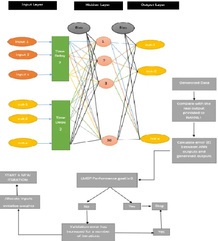
where 𝑋𝑡 and 𝑋𝑝𝑡 are the real and predicted values at time t respectively. The resulting NARNET and NARXNET structures with a flowchart of the LMBPA are shown in Figures 4 and 5 respectively.
Figure 5. NARXNET structure
3.5 MULTISTEP PREDICTIONS WITH NARNET AND NARXNET
In this research, one-, two-, three- and six-month ahead predictions are performed. The employed ANNs (NARNET and NARXNET) are utilised to make multi-step predictions, by transforming the networks from open-loop to closed-loop modes. Dynamic networks are with feedback, and transformation between the two modes is possible. Network training is performed with the selected time-series data, in open-loop mode and then transformed into the closed-loop mode, to continue the simulation for the desired predictions in the future.
Figures 6 and 7 represent the NARNET architecture, for one step ahead and multi-step ahead predictions respectively.
Source: MATLAB17a
Figure 7. NARNET closed-loop mode for multistep ahead prediction
Source: MATLAB17a
In the NARXNET model, the network is simulated in open-loop (series-parallel) mode, as long as there is known output. It is then transformed into closed loop (parallel) mode, to perform multi-step predictions, while providing only external input data (the exogenous variable). Therefore, all except the number of time steps, which have to be predicted, are provided to simulate the network in series-parallel mode. Then, only the time steps of the exogenous variable are used to simulate the network, in closed-loop form, and do the multi-step ahead predictions. Figures 8 and 9 represent the NARXNET architecture for one step and multi-step ahead predictions respectively.
Figure 8 NARXNET model for one-step ahead predictions
Source: MATLAB17a
Figure 9. NARXNET model in closed-loop mode for multistep predictions
Source: MATLAB17a
4. PRIMARY DATA AND DESCRIPTIVE DATA ANALYSIS
In order to analyse how and to what extent FFAs can improve forecasting performance, we use historical time series data on BPI and FFA prices. While BPI data is available online (free access),
FFA data has been provided by the Baltic Exchange and Lloyd’s List, in the form of daily FFA prices. The Baltic Exchange has provided data for all Panamax routes, for the period January 2013 to June 2016: P1A(P1E) Transpacific round voyage; P2A(P2E) Continent trip Far East; P3A(P3E) Transpacific round voyage; and P4TC Panamax Timechater average of the four routes of Skaw-Gibraltar transatlantic round voyage, Skaw-Skaw-Gibraltar trip to Taiwan-Japan, Japan–South Korea transpacific round voyage, and Japan-South Korea trip to Skaw Passero. The following settlements have also been provided by the Baltic Exchange: PCURMON; +1MON; +2MON; +3MON; P+2Q.
The Baltic Exchange data is used here, since it reflects the information provided by the panellists, and it is consistent with what BPI represents. The settlement periods provided by the Baltic Exchange match our needs, where one- to six-months ahead forecasts are carried out. The Panamax Index has been used because a) BFA for the BDI is not traded; b) the BFA Panamax (4 TC) is one of the most traded FFAs. BPI is the weighted average of the 4 time-charter Panamax routes (BPI 1A_03, BPI 2A_03, BPI 3A_03 and BPI 4A_03) and thus the corresponding BFA Panamax is the BFA P4TC, which is used in this paper. The BPI is available online for the period January 2009 to March 2017 (BPI, 2017).
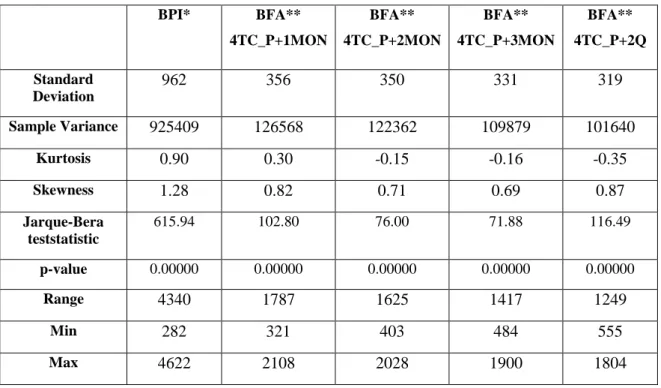
The summary statistics of BPI, BFA Panamax + 1MON, BFA Panamax + 2MON, BFA Panamax + 3MON and BFA Panamax + 6MON (2Q) are presented in Table 1.
Table 1 Primary Data Descriptive Statistics
BPI* BFA** 4TC_P+1MON BFA** 4TC_P+2MON BFA** 4TC_P+3MON BFA** 4TC_P+2Q Standard Deviation 962 356 350 331 319 Sample Variance 925409 126568 122362 109879 101640 Kurtosis 0.90 0.30 -0.15 -0.16 -0.35 Skewness 1.28 0.82 0.71 0.69 0.87 Jarque-Bera teststatistic 615.94 102.80 76.00 71.88 116.49 p-value 0.00000 0.00000 0.00000 0.00000 0.00000 Range 4340 1787 1625 1417 1249 Min 282 321 403 484 555 Max 4622 2108 2028 1900 1804
Count 1996 885 885 885 885
* BPI data were from Jan 2009 to March 2017 ** BFA data were from Jan 2013 to June 2016
*** BPI data were used in the NARNET model while BFA, together with BPI, were used in NARXNET to test the increased accuracy of the addition of BFA. Forecasting accuracy is measured by MSE using the data (i.e. forecasted data and settlement data) in the same periods.
It is interesting to observe that values of both standard deviation and sample variance decrease gradually from BFA 4TC_P+1MON to BFA 4TC_P+2Q. This implies that BPI volatility is difficult to predict, since BFA 4TC_P+1MON to BFA 4TC_P+2Q reflect market participants’ expectations from one to six months ahead. Skewness is significantly different from zero, and the distribution of all five datasets is right-skewed or positively-skewed. BPI skewness is greater than one, which means that the distribution is far from symmetrical. The values of the kurtosis are negative for BFA 4TC_P+2MON to BFA 4TC_P+2Q, implying a flatter distribution than the normal distribution for these datasets. For BPI and BFA 4TC_P+1MON, however, the kurtosis is positive, which means that the distribution of these two datasets is more peaked than the normal distribution. Higher kurtosis also means that more results of variance are derived from infrequent extreme deviations, as opposed to frequent, modestly-sized deviations. The Jarque-Bera test statistic and its p-value, calculated in Excel using CHISQ.DIST.RT (Jarque-Bera value, 2), where 2 is the degree of freedom, reconfirms that the data is not normally distributed for any of the time-series. These complexities necessitate the use of a non-linear tool, like ANNs, for forecasting future freight rates.
5. RESULTS
5.1 NARNET’S AND NARXNET’S PERFORMANCE
Forecasting accuracy has been assessed by calculating the MSE. The predicted values for the BPI are directly compared with the post-sample data. Before recording the post-sample (multistep) forecasts, the models have been retrained, until reaching the best performance. The results of both models reflect the multi-step performances, reached with 10, 20, 30, 40 and 50 neurons in the hidden layer (Table 4).
10 NEURONS 20 NEURONS 30 NEURONS 40 NEURONS 50 NEURONS NARNET (1) 6574.474 1624.879 381.7666 189.0927 218.417 NARNET (2) 22761.89 9243.433 4886.957 8349.553 NARNET (3) 26579.71 6082.726 5595.668 15736.24 NARNET (6) 144109.4 85022.54 80005.15 95008.92 NARXNET (1) 813.6734 239.8962 86.743 1430.5 NARXNET (2) 10824 7142.9 2800 2099.7 4209.9 NARXNET (3) 15438 3684.6 3188.6 8411.8 NARXNET (6) 129450 58753 13404 24095
There is an obvious tendency of the MSE increasing, as the forecasting horizon increases, in both models. It means that the result accuracy of short-term shipping freight forecasting is in general better than long-terms ones. Another important trend is that the MSE decreases in all models, usually reaching its lowest level in models with 30 neurons in the hidden layer. The models perform the worst with 10 neurons and best with 30 or 40 neurons, in the hidden layer. The models that performed better with 40 neurons, compared to 30 neurons, are NARNET (1) and NARXNET (2); these have been trained with 50 neurons as well, but the MSE increased in both.From Figure 10, it can be seen that, overall, the best performance is reached with 30 neurons in the hidden layer. The ordinate presents the value of MSE, while the axis shows the corresponding number of neurons (Figure 10). The MSE for each number of neurons is estimated as the average of the MSEs reached, in both models, for all forecasted horizons. It reveals that when using ANNs in shipping freight rate forecasting, the optimal number of the used neurons should be between 30 and 40, but with a higher likelihood at 30.
Figure 10. Validation of the number of neurons in the hidden layer
Figures 11 -14 plot the predicted values, with NARNET (30) and NARXNET (30), against the accurate values of the BPI. One-month ahead predictions are presented in Figure 11. It can be seen that both models, NARNET and NARXNET, perform quite well. They are able to predict the initial direction of the post-sample data. A better performance is reached by NARXNET (30), as the model produces better forecasts for the first half of the month, and then the forecasts slightly deteriorate; however, it remains a better shape compared with NARNET (30). It discloses that in the shipping freight rate forecasting of one month ahead, using BPI data only or using the combination of BPI and FFAs can deliver reliable forecasting results. However, the incorporation of FFAs can provide a better result compared to the case of using BPI data solely, particularly in the first half (i.e. 15 days) of the prediction period. 0.00E+00 5.00E+03 1.00E+04 1.50E+04 2.00E+04 2.50E+04 3.00E+04 3.50E+04 4.00E+04 4.50E+04 5.00E+04
10 NEURONS 20 NEURONS 30 NEURONS 40 NEURONS
MSE
v
alu
e
Validation of the number of neurons in the
hidden layer
Figure 11 One-month ahead predictions
Figure 12 shows predictions of two-months ahead. The prediction capability of both models is reduced, compared to the 1-month ahead predictions. Both models predict correctly the initial direction of the BPI. Again, NARXNET (30) outperforms NARNET (30) in this first stage. The models converge at the 24th step and after that NARXNET still predicts correctly the direction
(decrease of BPI) and the subsequent slight increase, while the NARNET (30) could not capture them. As a result, NARXNET (30) outperforms NARNET (30), with around 75%, with respect to MSE. It indicates that in the shipping freight rate forecasting of two months ahead, the result accuracy decreases compared to the case of one month ahead in general. However, the addition of FFA data in the forecasting model can significantly increase result accuracy.
400 450 500 550 600 650 700 750 800 1 2 3 4 5 6 7 8 9 10 11 12 13 14 15 16 17 18 19 20 21 22 23 24 25 In d ex Valu e Days
1-month ahead predictions
Figure 12. Two-month ahead predictions
Three-month ahead predictions are shown in Figure 13. Neither model is able to produce well the general pattern shown in the post-sample data, nor to predict correctly the peaks and troughs. Nevertheless, NARXNET (30) moves closer to the real values. Within the context of shipping freight rate analysis, having FFA data in the forecasting model of three months ahead can help improve the forecasting result accuracy, but not to a significant level.
Figure 13. Three-month ahead predictions
Figure 14 shows the results for six-month ahead predictions. NARXNET (30) was able to produce, partly, the overall pattern of the post-sample data, with its peaks and troughs. The model also
400 500 600 700 800 900 1000 1 3 5 7 9 11 13 15 17 19 21 23 25 27 29 31 33 35 37 39 41 43 45 In d ex Valu e Days
2-month ahead predictions
REAL VALUE NARNET (30) NARXNET (30)
400 500 600 700 800 900 1000 1 3 5 7 9 1113151719212325272931333537394143454749515355575961 In d ex Valu e Days
3-month ahead predictions
predicted the peak and the subsequent trough at the end of the forecasted period. Although NARNET (30) predicted better the initial direction of the BPI, its overall performance was around five times worse, w.r.t. MSE. It is clear that NARNET (30) could not predict either any of the peaks or troughs, or the general pattern of the post-sample data when the forecasting horizon increased to 6 months. We find that only using historical BPI data cannot provide any useful insight in the shipping freight rata forecasting of six months ahead. However, when the FFA data is combined with historical BPI, the model of six months ahead can better predict the general pattern (e.g. the peaks and troughs) of future freight rates for guiding ship-owners/charterers’ investments.
Figure 14. Six-month ahead prediction ns
ANNs’ performance and regression plots, for all the scenarios, are also analysed. The optimal number of epochs indicates the iteration at which the validation performance reached a minimum, and stopped training before over-fitting. The regression plot represents a linear regression between the outputs and the corresponding targets in the open-loop mode during an ANN training process. The outputs match the targets perfectly in open-loop mode, because in all models and all sets (training, validation and test) the R-value (correlation coefficient) was ≥ 0.99. Based on the results from Figures 11, 12 and 13, there is no significant evidence that NARXNET performs significantly better than NARNET, especially for forecasts of one-, two- and three months ahead. A significantly better forecast, however, is generated for six-months-ahead predictions. The analysis of the results from Figures 11-14 shows that having BFA data in addition to BPI can help improve forecasting accuracy, in the longer term
400 600 800 1000 1200 1400 1600 1800 1 6 11 16 21 26 31 36 41 46 51 56 61 66 71 76 81 86 91 96 101 106 111 116 121 126 In d ex Valu e Days
6-month ahead predictions
(i.e. 6 months), whenever BPI data alone does not work at all (indicated by a flat line in figure 14), and its impact in shorter terms (i.e. 1-3 months) is not significant.
5.2 INTERPRETATION OF THE RESULTS
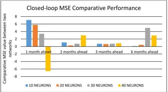
In nearly all experiments, NARXNET provided better results compared to NARNET. As expected, forecasting accuracy weakened as the forecast horizon increased. We prove, in a quantitative form, that having FFA in addition to BPI in shipping freight rate forecasting can improve the freight rate prediction accuracy, particularly in the case of six months ahead. The relative performance of NARXNET, compared to NARNET, decreased too, as the forecast horizon increased (Figure 15). Figure 15 presents the MSE relationship between the two models. NARNET’s MSE with 10 neurons was more than seven times higher, compared to NARXNET’s MSE. For one month ahead predictions, it is clear that the performance gap decreases as the number of neurons increases in both models. Moreover, NARNET (40) outperforms NARXNET (40) in one month ahead predictions. In the shipping freight rate forecasting of one month ahead, the stakeholders are suggested to use 40 neurons in their ANNs to reach the best forecasting results. Figure 15 also presents the correlation between inputs and outputs of the NARXNET model. The highest correlation, as expected, is for the inputs and outputs used for one month ahead predictions. The performances with 10, 20 and 30 neurons, for one-month ahead predictions, are in line with the assumption that, if cross-correlation between inputs and outputs is significant, NARXNET performs better. Although the best performance is reached with NARXNET (30) – 1, correlation between inputs and outputs will not always guarantee better results for NARXNET, as NARNET (40) – 1 outperformed NARXNET (40) - 1. This also suggests that, for short-term forecasts, NARNET can predict as accurately as NARXNET, subject to more neurons in the hidden layer. It is evidenced that in shipping freight rate forecasting of one month ahead, FFA data does not carry a heavy weight to improve forecasting freight rate accuracy. In this case, ship-owners and charterers shall take into account that the key factor lies in the use of a high number of neurons (i.e. 40) in the hidden layer in ANNs. For two-month ahead predictions, the performance gap decreases and so does the correlation between inputs and outputs. The biggest performance gap is observed with 40 neurons and the lowest with 20. This implies that the existing correlation, between inputs and outputs, does not allow NARXNET to outperform NARNET significantly, and changing the number of neurons did not reveal any general trend. Different with the forecasting of one month ahead, the number of used neurons in ANNs plays an insignificant role
in improving freight rate prediction accuracy. The analysis result suggests that the stakeholders can simply rely on BPI data only in the ANN forecasting model; and the number of neurons has very limited effect on the forecasting accuracy, though using 30 neurons can very marginally outperform the others. With regard to three-month ahead predictions, the performance gap between the models decreased further, and so did the correlation between inputs and outputs. Interestingly, nearly the same performance gap was observed with different numbers of neurons. The latter suggests that increasing the number of neurons in the hidden layer does not help the networks to perform better with low correlation between inputs and outputs. For six months ahead predictions, the correlation between inputs and outputs decreased significantly to 0.01, and so did the performance gap, with 10 and 20 neurons. However, NARXNET with 30 neurons generated unexpectedly good forecasts, despite the low correlation between inputs and outputs. After comparison between the inputs in closed-loop mode and the forecasted outputs, a considerably higher correlation was discovered at 0.49; this partially explains the obtained good forecasts.
Figure 15 MSE Comparative Performance
The outcome of our experiments supports similar findings from previous studies, as described below. Our results are not only relevant, with regard to FFAs and their potential for increasing forecasting accuracy, but also with regard to the incorporation of exogenous variables, containing useful information, in forecasting models. The outcome quantitatively proves many statements in the relevant literature. For instance, the results support (Zhang et al., 2014), who have suggested that the incorporation of FFA prices could improve the forecasting performance of models, aiming at predicting future spot rates in the short-term. Batchelor et al. (2007) also stated that future freight
-8 -6 -4 -2 0 2 4 6 8
1 month ahead 2 months ahead 3 months ahead 6 months ahead
Com p ar at iv e MSE v alu e b etwe en two n etwork s
Closed-loop MSE Comparative Performance
rates help to forecast future spot rates. In relation to this, albeit earlier, Kavussanos and Visvikis (2004) have demonstrated that FFAs have a similar feature to that of derivatives contracts in commodity and financial markets, and thus they can be used as a price-discovery tool. The correlation analysis in our study mirrors such findings. It also supports Kasimati and Veraros (2017), in which the ability of FFAs to forecast, in the longer-term, was considered to be of limited value. In our study, the MSE values of NARXNET increase considerably, as the forecast horizon increases, nearly 154 times (from 86.743 to 13404). Our findings also show certain differences with previous studies. For example, Kasimati and Veraros (2017) emphasised that FFAs cannot capture the turning points of the direction of freight rate movements. From Figures 11-15, our results indicate that, by employing ANNs, these turning points can be captured. The incorporation of FFA information in freight rate forecasting shows the importance of additional market information in improving forecasting accuracy. This mirrors the findings of Tsioumas et al. (2017), where forecasting improved by employing additional market information (Dry Bulk Economic Climate Index) in a VARX model. Overall, our results confirm that the incorporation of FFA information enhances forecasting accuracy. From the practical managerial perspective, shipowners can use FFA for traditional risk management (e.g. hedging), as well as new freight rate forecasting for exploring better business opportunities.
6. Conclusions
Baltic Indices are important to shipping market participants, as they reflect an assessment of the cost of sea-borne transport services, on different routes and types of vessels. The movement of the BDI and its constituent indices is highly volatile and depends on many variables (e.g. vessel size and age, bunker price, length and severity of global economic winters, and cyclicality), as well as on the peculiarities of the freight market mechanism (i.e. the equilibrium between demand and supply of shipping). This suggests that the forecasting of the Baltic Indices is a complex task, necessitating the application of complex techniques. We have used two different ANNs to generate forecasts; they are highly accurate for one-month ahead predictions, gradually deteriorating as the forecast horizon increases. In general, NARXNET out-performs NARNET. This means that, by using market information, the NARXNET FFA forecasts are better than the NARNET model, purely on the basis of historical data.
The results of the forecasting experiment reconfirm that the information contained in FFAs can improve forecasting accuracy. This has practical implications. As FFA prices are available for a
certain period -one, two, three and six months-, market participants can obtain better forecasts and thus have better insight into future movements in the freight market. Moreover, as participants in the FFA market are diverse, compared to participants in the spot market, the speculative activity on FFA price formation incorporates valid information on future freight market movements, and justifies that, in a speculatively efficient derivatives market, the price discovery function of derivatives is more prominent. Nowadays, one of the most valuable assets is information and the speed of its transmission, which suggests that participants or companies that can make the maximum use of relevant sources of information, at any given time, have the chance of being more successful than their competitors. The findings of this paper contribute to knowledge in this regard. To further investigate the advantages of our proposed models, it would be beneficial to compare our results, with those obtained by other models (e.g. VECM, ARIMA) in future.
ACKNOWLEDGEMENTS
The authors thank the anonymous reviewers and the Editor in Chief of MEL for their valuable comments, from both technical and grammatical perspectives, to improve the quality of this paper. REFERENCES
1. Bao, J., Pan, L. and Xie, Y. (2016) ‘A new BDI forecasting model based on support vector machine’, 2016 IEEE Information Technology, Networking, Electronic and Automation Control Conference Information Technology, Networking, Electronic and Automation Control Conference, IEEE. :65-69
2. Batchelor, R. A., Alizadeh, A. H. and Visvikis, I. D. (2007) ‘Forecasting spot and forward prices in the international freight market’, International Journal of Forecasting, 23(1), pp.101-114
3. Bessler, W., Drobetz, W. and Seidel, J. (2008) ‘Ship funds as a new asset class: An empirical analysis of the relationship between spot and forward prices in the freight markets’, Journal of Asset Management, 9(2), pp.102-120
4. BPI (2017). Available at:
https://www.quandl.com/data/LLOYDS/BPI-Baltic-Panamax-Index [Accessed: 2 March 2017]
5. Chen, S., Meersman, H. and von de Voorde, E. (2012) ‘Forecasting spot freight rates at main routes in the dry bulk market’, Maritime Economics & Logistics, 14(4), pp.498-537 6. Duru, O. (2010) ‘A fuzzy integrated logical forecasting model for dry bulk shipping index
forecasting: An improved fuzzy time series approach’, Expert Systems With Application,
37(7), pp.5372-5380
7. Duru, O. and Yoshida, S. (2009) ‘Judgmental Forecasting in the Dry Bulk Shipping Business: statistical vs. Judgmental Approach’, The Asian Journal of Shipping and Logistics, 25(2), pp.189-217
8. Duru, O., Bulut, E. and Yoshida, S. (2010) ‘Bivariate Long Term Fuzzy Time Series Forecasting of Dry Cargo Freight Rates’, The Asian Journal of Shipping and Logistics,
9. Gavin, H.P. (2017) The Levenberg-Marquardt method for nonlinear least squares curve-fitting problems. Available at: http://people.duke.edu/~hpgavin/ce281/lm.pdf. [Accessed: 5 August 2017]
10. Gavriilidis, K., Kambouroudis, D., Tsakou, K. and Tsouknidis, D. (2018) ‘Volatility forecasting across tanker freight rates: The role of oil price shocks’, Transportation Research Part E-Logistics and Transportation Review, 118, pp. 376-391
11.Ghiassi, M., Saidane, H. and Zimbra, D. K. (2005) ‘A dynamic artificial neural network model for forecasting time series events’, International Journal of Forecasting, 21(2), pp.341-363
12.Gong, X. and Lu, J. (2016) ‘Volatility Spillovers in Capesize Forward Freight Agreement Markets’, Scientific Programming, pp.1-8
13.Ghiassi, M. and Nangoy, S. (2009) ‘A dynamic artificial neural network model for forecasting nonlinear processes’, Computer & Industrial Engineering, 57(1). pp.287-297 14.Hagan, M.T., Demuth, H.B., Beale, M.H. and De Jesus, O. (2014) Neural Network Design.
2nd ed. Available at: http://hagan.okstate.edu/NNDesign.pdf. [Accessed: 5 March 2017] 15.Kasimati, E. and Veraros, N. (2017) ‘Accuracy of forward freight agreements in forecasting
future freight rates’, Applied Economics, pp. 1-14
16.Kavussanos, M. G. (1996) ‘Comparisons of Volatility in the Dry-Cargo Ship Sector: Spot versus Time Charters, and Smaller versus Larger Vessels’, Journal of Transport Economics and Policy, 30(1), pp.67-82
17.Kavussanos, M. G. and Alizadeh, A. H. (2001) ‘Seasonality patterns in dry bulk shipping spot and time charter freight rates’, Transportation Research Part E, 37(6), pp.443-467 18.Kavussanos, M. G. and Nomikos, N. K. (2003) ‘Price Discovery, Causality and Forecasting
in the freight Futures Market’, Review of Derivatives Research, 6(3), pp.203-230
19.Kavussanos, M. G. and Visvikis, I. D (2004) ‘Market interactions in returns and volatilities between spot and forward shipping freight markets‘, Journal of Banking and Finance, 28(8), pp.2015-2049
20.Kavussanos, M. G., Visvikis, I. D. and Menachof, D. (2004) ‘The Unbiasedness Hypothesis in the Freight Forward Market: Evidence from Cointegration Tests’, Review of Derivatives Research, 7(3), pp.241-266
21.Kavussanos, M. G., Visvikis, I. D. and Dimitrakopoulos, D. (2010) ‘Information linkages between Panamax freight derivatives and commodity derivatives markets’, Maritime Economics & Logistics, 12(1), pp.91-110
22.Kisi, O and Uncuoglu, E. (2005) ‘Comparison of three back-propagation training algorithms for two case studies’ , Indian Journal of Engineering & Materials Sciences, 12, pp.434-442 23.Leonov, Y. and Nikolov, V. (2012) ‘A wavelet and neural network model for the prediction
of dry bulk shipping indices’, Maritime Economics & Logistics, 14(3), pp.319-333
24.Li, J. and Parsons, M. G. (1997) ‘Forecasting freight rate using neural networks’, Maritime Policy & Management, 24(1), pp.9-30
25.Li, K., Qi, G., Shi, W., Yang, Z., Bang, H., Woo, H. and Yip, T. (2014) ‘Spillover effects and dynamic correlations between spot and forward tanker freight markets’, Maritime Policy & Management, 41(7), pp.683-696
26. Lourakis, M. (2005) A Brief Description of the Levenberg-Marquardt Algorithm
Implemented by levmar. Available at: http://users.ics.forth.gr/~lourakis/levmar/levmar.pdf. [Accessed: 18 August 2017]
27.Lyridis, D.V., Zacharioudakis, P., Mitrou, P. and Mylonas, (2004) ‘Forecasting Tanker Market Using Artificial Neural Networks’, Maritime Economics & Logistics, 6(2), pp.93-108
28.Lyridis, D., Zacharioudakis, P., Iordanis, S. and Daleziou, S. (2013) ‘Freight-Forward Agreement Time series Modelling Based on Artificial Neural Network Models’, Journal of Mechanical Engineering, 59(9), pp.511-516
29.Montgomery, D.C., Jennings, C. L. and Kulahci, M. (2015) Introduction to time series analysis and forecasting 2nd ed. NJ: Wiley
30.Munim, Z and Schramm, H. (2017) ‘Forecasting container shipping freight rates for the Far East - Northern Europe trade lane’, Maritime Economics & Logistics, 19(1), pp. 106-125 31.Nasr Mahmoud S., Moustafa Medhat, A.E., Seif Hamdy A.E. and El Kobrosy, G. (2012)
‘Application of Artificial Neural network (ANN) for the Prediction of EL-AGAMY
wastewater treatment plant performance-EGYPT’, Alexandria Engineering Journal, 51(1), pp.37-43
32.Nomikos, N.K. and Doctor, K. (2013) ‘Economic significance of market timing rules in the Forward Freight Agreement markets’, Transportation Research: Part E, 52, pp.77-94 33.NN Toolbox, 2017. Available at:
https://www.mathworks.com/products/neural-network.html.[Accessed: 5 March 2017]
34.Oancea, B. and Ciucu, S.K. (2013) ‘Time Series Forecasting Using Neural Networks’,
Challenges of the Knowledge Society, 3, pp.1402-1408
35.Papailias, F., Thomakos, D. D. and Liu, J. (2017) ‘The Baltic Dry Index: cyclicalities, forecasting and hedging strategies’, Empirical Economics, 52(1), pp. 255-282
36.Patil, K., Deo, M.C., Ghosh, S. and Ravichandran, M. (2013) ‘Predicting Sea Surface Temperatures in the North Indian Ocean with Nonlinear Autoregressive Neural Networks’,
International Journal of Oceonagraphy, pp.1-12
37.Randers, J. and Goluke, U. (2007) ‘Forecasting turning points in shipping freight rates: lessons from 30 years of practical effort’, System Dynamics Review, 23(2-3), pp. 253-284 38.Sapna, S. (2012) ‘Backpropagation Learning Algorithm Based on Levenberg Marquardt
Algorithm’, The Fourth International Workshops on Computer Network & Communications, 26th to 28th October. Coimbatore, India
39.Santos, A.A.P., Junkes, L.N. and Pires Jr, F.C.M (2014) ‘Forecasting period charter rates of VLCC tankers through neural networks: A comparison of alternative approaches’, Maritime Economics and Logistics, 16(1), pp.72-91
40.Stopford, M. (2009) Maritime Economics. 3rd ed. London: Routledge
41.Sudhakaran, P., Vel Murugan, V., Sivasakthivel, P.S. and Balaji, M. (2011) ‘Prediction and optimization of depth of penetration for stainless steel gas tungsten arc welded plates using artificial neural networks and simulated annealing algorithm’, Neural Computing and Applications, 22(3), pp.637-649
42.Tsioumas, V. and Papadimitriou, S. (2015) ‘Chinese steel production and shipping freight markets: A causality analysis’, International Journal of Business & Economic Development,
3(2), pp.116-124
43.Tsioumas, V. and Papadimitriou, S. (2016) ‘The dynamic relationship between freight markets and commodity prices revealed’, Maritime Economics and Logistics, pp.1-13 44.Tsioumas, V., Papadimitriou, S., Smirlis, Y. and Zahra, S. Z. (2017) ‘A Novel Approach to
Forecasting the Bulk Freight Market’, Asian Journal of Shipping and Logistics, 33(1), pp.33-41
45. UNCTAD (2016) Review of Maritime Transport 2016. Available at:
http://unctad.org/en/PublicationsLibrary/rmt2016_en.pdf. [Accessed: 2 March 2017]
46.Uyar, K., Ilhan, Ü. and Ilhan, A. (2016) ‘Long Term Dry Cargo Freight Rates Forecasting by Using Recurrent Fuzzy Neural Networks’, Procedia Computer Science, 102:642-647
47.Veenstra, A. W. and Franses, P. H. (1997) ‘A co-integration approach to forecasting freight rates in the dry bulk shipping sector’, Transportation Research Part A: Policy & Practice,
31(6), pp.447-459
48.Veenstra, A. W. and Haralambides, H. E. (2001) ‘Multivariate autoregressive moels for forecasting seaborne trade flows’, Transportation Research Part E, 37(4), pp.311-319
49. Visvikis, I. D. (2002) An econometric analysis of the forward freight market. Available at:
http://openaccess.city.ac.uk/7596/. [Accessed: 01 March 2017]
50.Wang, H., Yan, X., Chen, H., Chen, C. and Guo, M. (2015) ‘Chlorophyll-A Predicting Model Based on Dynamic Neural Network’, Applied Artificial Intelligence, 29(10), pp.962-979
51.Yu, L., Yang, Z. and tang, L. (2017) ‘Ensemble Forecasting for Complex Time Series Using Sparse Representation and Neural Networks’, Journal of Forecasting, 36(2), pp.122-139 52.Zeng, Q., Qu, C., Ng, A.K.Y. and Zhao, X. (2016) ‘A new approach for Baltic Dry Index
forecasting based on empirical mode decomposition and neural networks’, Maritime Economics & Logistics, 18(2), pp.192-210
53.Zhang, G., Patuwo, E.B. and Hu, M.Y. (1998) ‘Forecasting with artificial neural networks: The state of the art’, International Journal of Forecasting, 14(1), pp.35-63
54.Zhang, J., Zheng, G. and Zhao, X. (2014) ‘Forecasting spot freight rates based on forward freight agreements and time charter contracts’, Applied Economics, 46(29), pp.3639-3648
Appendix 1. Static and Dynamic ANNs
Neural networks (NNs) can be classified as static and dynamic. In static NNs, the outcome is calculated instantly from the input data through feedforward connections while, in dynamic NNs, the output depends on both the current and the previous inputs (Hagan et al., 2014). Consequently, dynamic networks, working on a sequence of inputs, which contain delays and have memory, are more powerful than static ones, when it comes to modelling complicated non-linear dynamic systems (Wang et al., 2015). In classical NNs, dynamic networks consist of an input, hidden and output layers. The input layer receives the data and then all observations are used to train the network (Ghiassi et al., 2005). Dynamic networks are data driven, feedforward, of multilayer dynamic architecture. They are formed according to the concepts of learning and acquiring knowledge, then propagating and modifying this knowledge forward, reiterating these steps until reaching the desired performance (Ghiassi and Nangoy, 2009). Dynamic networks are used in this paper, because freight rate prediction is a form of dynamic filtering, where both historical rates and FFA information are used simultaneously in the model.
In order to analyse the forecasting performance of FFAs, two different models of dynamic NNs are employed and compared. Firstly, both NN models have to be trained and the values of connection
weights and bias are estimated through a training algorithm (Patil et al., 2013). Training continues until training error between target and calculated outputs reaches the error goal, or until no further reduction in the error is achieved (Patil et al., 2013). The fundamental element of NN is the neuron, or node in Figure 1. Inputs are represented by 𝑎𝑖 and the output by 𝑂𝑗. The neuron processes these inputs and finishes with a single output signal. Every input is multiplied by its corresponding weight,
𝑊𝑖,𝑗and the neuron uses the sum of these weighted inputs and adds the bias 𝑏𝑗 (i.e. the node’s internal threshold). The bias is a randomly chosen value that determines the node’s net input in Eq (1):
𝑢𝑗 = ∑𝑛𝑖=1(𝑊𝑖,𝑗∗ 𝑎𝑖) + 𝑏𝑗 (1)
Then, the neuron processes the sum through a transfer function and produces the output value 𝑂𝑗 of the neuron (Nasr Mahmoud et al., 2012).
Figure 1 Single node anatomy
Source: Nasr Mahmoud et al. (2012)
Activation functions, defining the output of a given neuron in the different layers of the network, can be different (e.g. sigmoid, hyperbolic or linear). In this paper, the linear transfer function is used for the output neuron, where the output of the function is equal to its input. The sigmoid transfer function is used for the hidden neurons, in the multi-layer networks, in order to generate their output. For the NARNET and NARXNET models, the tan-sigmoidal transfer function is used. This function takes the input, which can be any value ∞, +∞] and squashes the output into the range [-1, 1]. The tan-sigmoidal transfer function is differentiable, which is a prerequisite for the training algorithm used; this provides a good compromise, where the speed of the NN is of critical