Non-parametric Bayesian models
for structured output prediction
Sébastien Bratières
King’s College
University of Cambridge
This dissertation is submitted for the degree of Doctor of Philosophy
Structured output prediction is a machine learning tasks in which an input object is not just assigned a single class, as in classification, but multiple, interdependent labels. This means that the presence or value of a given label affects the other labels, for instance in text labelling problems, where output labels are applied to each word, and their interdependencies must be modelled.
Non-parametric Bayesian (NPB) techniques are probabilistic modelling tech-niques which have the interesting property of allowing model capacity to grow, in a controllable way, with data complexity, while maintaining the advantages of Bayesian modelling. In this thesis, we develop NPB algorithms to solve structured output prob-lems.
We first study a map-reduce implementation of a stochastic inference method de-signed for the infinite hidden Markov model, applied to a computational linguistics task, part-of-speech tagging. We show that mainstream map-reduce frameworks do not easily support highly iterative algorithms.
The main contribution of this thesis consists in a conceptually novel discriminat-ive model, GPstruct. It is motivated by labelling tasks, and combines attractdiscriminat-ive prop-erties of conditional random fields (CRF), structured support vector machines, and Gaussian process (GP) classifiers. In probabilistic terms, GPstruct combines a CRF likelihood with a GP prior on factors; it can also be described as a Bayesian kernel-ized CRF.
To train this model, we develop a Markov chain Monte Carlo algorithm based on elliptical slice sampling and investigate its properties. We then validate it on real data experiments, and explore two topologies: sequence output with text labelling tasks, and grid output with semantic segmentation of images. The latter case poses scalab-ility issues, which are addressed using likelihood approximations and an ensemble method which allows distributed inference and prediction.
The experimental validation demonstrates: (a) the model is flexible and its con-stituent parts are modular and easy to engineer; (b) predictive performance and, most crucially, the probabilistic calibration of predictions are better than or equal to that of competitor models, and (c) model hyperparameters can be learnt from data.
This dissertation is the result of my own work and includes nothing which is the outcome of work done in collaboration except as declared in the Preface and specified in the text.
It is not substantially the same as any that I have submitted, or, is being concur-rently submitted for a degree or diploma or other qualification at the University of Cambridge or any other University or similar institution except as declared in the Preface and specified in the text. I further state that no substantial part of my disser-tation has already been submitted, or, is being concurrently submitted for any such degree, diploma or other qualification at the University of Cambridge or any other University or similar institution except as declared in the Preface and specified in the text
It does not exceed sixty-five thousand words in length, and contains no more than hundred fifty figures.
I would like to express my sincere gratitude to my supervisor Zoubin Ghahramani for his continuous support and his patient, steady and insightful guidance over the course of my research. Like many in our research group, I have found inspiration in Zoubin’s ability to boil down complex machine learning notions to their simplest accurate explanation. Over the years, Zoubin made it a speciality to represent rela-tionships between machine learning concepts with graph metaphors, and figure 3.2.1 in this thesis bears witness to this influence.
This thesis would not have been possible without the support, intellectual stim-ulation and friendships offered by my research group. In particular, I wish to thank Zoubin and Carl Rasmussen, my adviser, for creating, shaping and fostering such a brilliant group as ours; one that excels from a scientific point of view but also provides a vibrant and supportive environment. Thanks to Diane Hazell, our group adminis-trator, for her unfailing help, and thanks to Sae and David Franklin, for the good time we had together. Thanks to Simon Lacoste-Julien, who sparked my interest for struc-tured output prediction and statistical learning methods which lie outside the group’s traditional scientific remit. I was fortunate to work with enthusiastic and knowledge-able co-authors: Jurgen, Andreas, Novi, Sebastian and Zoubin; Novi’s drive and per-severance in particular allowed many of the ideas on GPstruct, the statistical model developed in this thesis, to come to fruition.
I chose to conduct my PhD research part-time, while working in industry, and am indebted to my two employers, Voice Insight and dawin gmbh, for they support, flexibility and trust.
“L’argent est le nerf de la guerre”, “Money is the sinew of war”, and accordingly, I would like to express my sincere gratitude to: Amazon for their generous spon-sorship, through two Amazon Educational Grants towards computing expenses, as well as for the expert advice provided by the Amazon Elastic MapReduce engineering team; Yahoo! for the funding provided through the Key Scientific Challenges Award; King’s College, the Department of Engineering and the Ford of Great Britain Trust for subsidising my conference trips; and my supervisor Zoubin Ghahramani for covering research and travel expenses from group resources on several occasions.
My parents, my sister, and my grand-parents, each according to their own charac-ter and life path, have been all of inspiration, encouragement and assistance at once. Finally, and most importantly, I would like to thank my wife Vittoria, for encour-aging me to return to Cambridge, for supporting me with patience, determination and loving advice throughout these years, in particular during the trying times, for keeping the home fires burning, and ultimately, for making the journey worthwhile.
List of figures 14
List of acronyms 15
1 Introduction 17
1.1 Motivation . . . 17
1.2 Thesis structure . . . 20
1.3 Notations and conventions . . . 22
2 Map-reduce inference for the infinite HMM 23 2.1 Sequence models and the IHMM . . . 24
2.1.1 Hidden Markov models, state space cardinality, clustering, and non-parametric Bayesian models . . . 24
2.1.2 Part-of-speech tagging . . . 26
2.1.3 Defining a non-parametric model for sequence observations . 27 2.1.4 The HDP-HMM . . . 31
2.2 Distributed computing aspects . . . 33
2.2.1 Commodity computing infrastructure . . . 33
2.2.2 Principle of map-reduce . . . 36
2.2.3 Map-reduce architecture for the PoS IHMM . . . 37
2.2.3.1 Data storage . . . 37
2.2.3.2 Details of MR jobs . . . 38
2.2.3.3 Dependency diagram . . . 39
2.2.4 MR job latency . . . 39
2.2.5 Use of a reference, non-distributed implementation . . . 43
2.3 Experiments . . . 44
2.3.1 Algorithm and data . . . 44
2.3.2 Configurations . . . 45
2.3.3 Results . . . 46
2.4 Iterative map-reduce . . . 49
2.4.1 Understanding of the issue in the community . . . 50 7
2.4.2 Fixing iterative map-reduce: today’s perspective . . . 51
2.4.2.1 Adapted map-reduce frameworks . . . 52
2.4.2.2 Beyond map-reduce . . . 53
2.5 Review of the state of the art for distributed probabilistic inference . 54 2.6 Conclusion . . . 58
3 Discriminative models for structured output prediction 61 3.1 From generative to discriminative modelling . . . 61
3.2 A roadmap . . . 63
3.3 Illustrating the roadmap: linear regression . . . 64
3.4 Making the model Bayesian . . . 66
3.5 Making the model kernelised . . . 67
3.6 Making the model structured . . . 70
3.7 The CRF model and extensions . . . 71
3.7.1 Variants of the CRF . . . 73
3.7.2 Maximum margin extensions of the CRF . . . 76
3.8 Conclusion . . . 78
4 GPstruct for sequence labelling 79 4.1 Model formulation . . . 80
4.2 Parameterisation for sequence problems . . . 81
4.3 Kernel function specification . . . 83
4.4 Inference procedures . . . 84
4.4.1 Predictive distribution . . . 84
4.4.2 Sampling from the posterior distribution . . . 85
4.5 Experiments: text processing tasks . . . 86
4.5.1 Train vs. test split . . . 87
4.5.2 Baselines . . . 87
4.5.3 Computing . . . 87
4.5.4 Results and interpretation . . . 88
4.6 Experiments: video processing task . . . 88
4.7 Practical issues . . . 89
4.8 Cross-chain MCMC variance . . . 91
4.9 Comparisons with existing models . . . 92
4.10 MAP variant of GPstruct . . . 96
4.10.1 Experiments . . . 97
4.11 Further GP models with structure . . . 97
4.11.1 Different definitions of “structure” for GP structured regression 100 4.12 Conclusion . . . 101
5 Scaling up GPstruct: pixel grid labelling 104
5.1 Grid parameterisation . . . 105
5.2 Approximations for scaling . . . 106
5.3 Algorithm . . . 109
5.3.1 Algorithm complexity . . . 109
5.4 Experimental setup . . . 110
5.4.1 Runtimes . . . 112
5.5 Experimental research questions and results . . . 112
5.5.1 What is the predictive performance of GPstruct? . . . 112
5.5.2 Are GPstruct’s predictions probabilistically calibrated? . . . . 113
5.5.3 Is GPstruct’s performance just due to bagging? . . . 115
5.5.4 What is the influence of varying the number of sampled pixels? 115 5.5.5 What is the impact of PL and TRW approximations? . . . 115
5.6 Scaling further . . . 117
5.6.1 Variational inference for GPstruct . . . 119
5.7 Conclusion . . . 121
6 Hyperparameter inference 122 6.1 Motivation . . . 122
6.2 Bayesian hyperparameter inference for GPstruct . . . 125
6.2.1 Canonical (forward) parameterisation . . . 126
6.2.2 Whitening the prior . . . 126
6.2.3 Surrogate data method . . . 127
6.2.4 Further variants . . . 128
6.3 Geweke’s “Getting it right” tests . . . 129
6.3.1 Our variant of the test . . . 131
6.3.2 Experiment: testing elliptical slice sampling implementation . 132 6.3.3 Experiment: testing hyperparameter sampling implementations 133 6.3.4 Hyperparameter learning: synthetic data experiment . . . 136
6.4 Experiments on NLP tasks . . . 139
6.4.1 Hyperparameter update runtime . . . 139
6.4.2 Applying ARD kernels to the NLP tasks . . . 139
6.4.3 Experimental configuration and results . . . 140
6.5 Conclusion . . . 151
7 Conclusion 155 7.1 Summary of scientific contributions . . . 155
7.2 Concluding thoughts . . . 157
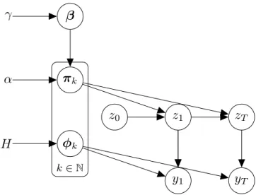
2.1.1 Various clustering and HMM models . . . 28 2.1.2 Graphical model of the IHMM. Rowsπk, k∈Nof the state transition
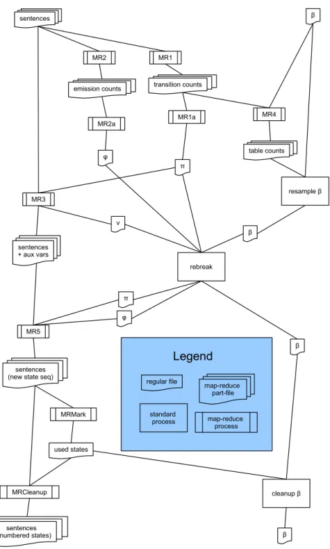
matrix are given a HDP prior. Cf. section 2.1.4 for a full description. 31 2.2.1 Dependency diagram for one MCMC iteration. “Regular files” are
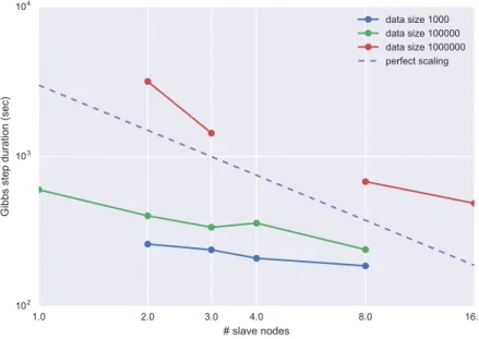
HDFS files. “Standard processes” are small tasks executed in-memory on the master node, possibly as Java for-loops. There is a se-quence of in-place modifications of the sentences (represented in vertical alignment) which traverses the following jobs: MR3, MR5, MRCleanupUsedStates. . . 41 2.3.1 hadoop-1experiments for selected data set sizes, with varying
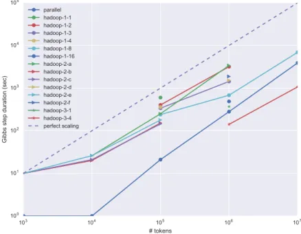
num-bers of slave nodes (x-axis logarithmic). If total computational cost of an experiment scaled linearly with the number of nodes (which is the optimum when distributing computation over a cluster), the lines would run parallel to the dashed line. However, they are more hori-zontal; this means that the Gibbs step duration does not decrease as much as desired. . . 46 2.3.2 Allhadoop-2-{a...f}experiments are duplicates of one another. This
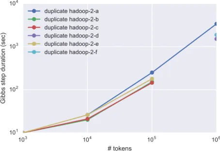
demonstrates that there is little variability between runs. . . 47 2.3.3 All experiments in the same plot. The general scaling trend follows
that of the parallel setup. Increasing data size even further than what was tested here, we expect that hadoop-1and hadoop-2setups will
become faster than theparallelsetup. However, the point where e.g.
lines for experimentshadoop-1-8andparallelintersect seems several
orders of magnitude above present experiments. Thehadoop-3
ex-periments demonstrate a setup which beats theparallelsetup, using
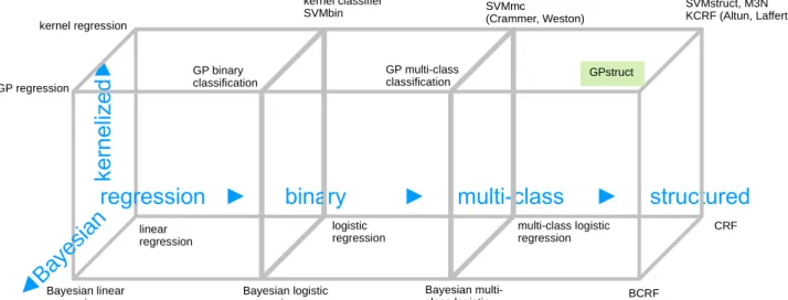
distribution and more powerful slave nodes. . . 48 3.2.1 An overview of some discriminative models in supervised learning.
(Author names in the figure are included to distinguish several vari-ants of a model) . . . 65
3.7.1 Graphical model for a CRF as a mixed (i.e. directed and undirected) graph, also called a partially directed graph. The MRF part specifies the dependencies insidey. Allytnodes depend onx, which may have
structure, but it is ignored here. . . 72 4.2.1 Factor graph for sequence prediction with two clique types,
un-ary location-dependent cliques ˜ct and binary location-independent
cliques˜˜c. Input nodes are always treated as observed. . . . 82 4.6.1 Error rate cross plot of the20gesture video sessions. The axes
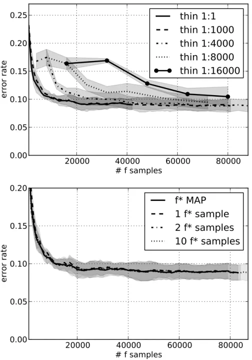
corres-pond to error rate of GPstruct with SE kernel and CRF, the diagonal line shows equal performance. The shadowed stars are those with at least5%performance difference. . . 89 4.7.1 Top: Effect of thinning, i.e. samplingf∗|f more rarely than everyf
sample. Chunkingtask,f∗MAP scheme,hb = 1. Bottom: Effect of
number off∗|f samples for eachf sample. Chunkingtask, thinning at 1:1 000,hb= 1. . . 90
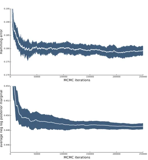
4.8.1 Mean and variance plots over 20 MCMC chains for HE and ANLPM metrics. . . 93 5.1.1 Grid factor graph with pairwise factors. There is one unary factor per
pixel (the observed variable nodes for thexthave been left out to not
crowd the picture), and one pairwise factor. . . 105 5.4.1 Semantic segmentation task. Example marginals (brightness level
en-codes certainty) and predicted labels from the Stanford Background Dataset. All methods use the same image features. First row: input image and true labels, second row: marginals and predicted labels ofindependent,third row: of CRF PL,fourth row: of CRF LBMO, fifth row: of GPstruct. Theindependentmodel performs reason-ably well in predicting per-pixel segmentation, but makes rather noisy predictions, whereasCRF PLputs more emphasis on pairwise factors resulting in large same-label patches in predictions. GPstruct com-bines the good per-pixel segmentation ofindependentand smooth-ness ofCRF PL. . . 113 5.5.1 Stanford Background Dataset: plot corresponding to table 5.1 (CRF
PL, whose results are much worse than the rest, is not represented). . 116 5.5.2 Quality of the posteriors, measured by the ANLPM metric. The
ex-perimental configuration is described in section 5.5.2. . . 116 5.5.3 Speed-accuracy trade-off for GPstruct and CRF LBMO bag. The
pixel-wise Hamming error is measured. The experimental configuration is the same as in section 5.5.2. . . 118
5.5.4 Effect of approximations in the standard GPstruct. All combinations of exact likelihood vs. PL and max-product prediction vs. TRW pre-diction are explored. The prepre-diction approximation has virtually no effect on performance (curves with exact max-product and TRW pre-diction overlap), and the likelihood approximation proves very robust. 118 6.1.1 Sketch of probabilistic model with latent variables and hyperparameters 124 6.3.1 Graphical model illustrating the successive-conditional procedure. . . 131 6.3.2 Diagnostic plots of Geweke experiment runs resulting in different
res-ults for the KS test. From top to bottom: not rejected, rejected but correct implementation, rejected due to faulty implementation. Each row is for a specific hyperparameter. Theleftplot shows the prior or empirical posterior distribution, therightplot shows the (empirical) cumulative distribution function. . . 135 6.3.3 Does hyperparameter learning help ignoring the noise features? Top:
Experiments with prior whitening vs. no hyperparameter sampling, showing influence of noise feature weight. Bottom: experiments with slice sampling, noise feature weightw = 10, showing the influence of the hyperparameter update rate. . . 137 6.3.4 Histogram of sample path for the log ARD variancesψ1...ψ5(signal
features, all collected in one set, in blue on the plot), andψ6...ψ10
(noise features, collected in another set, in green on the plot). The con-figurations considered are: top, PW; bottom, SS. In both cases, noise feature weightw= 10, and hyperparameter update rate is 1 every 10 ESS steps. The values of the hyperparameter were binned into 10 bins of equal width over their range. . . 138 6.4.1 Plot of values ofdiag(XTX)whereXis the feature matrix. If we
de-cide to try and identify 5 boundary points between features of similar covariance, we can choose the following values: 252, 522, 732, 852, 1186. 141 6.4.2 Experiment: learning the linear kernel’s binary scaling
hyperpara-meter hb (represented asloghb). Hyperparameter set: just loghb.
Hyperpriorloghb ∼ U(log 10−3,log 102). Initial valueloghb = 0.
Sampling hyperparameters every 1 000 latent variable updates. Dif-ferent configurations: difDif-ferent NLP tasks; hyperparameter updates using slice sampling or prior whitening. . . 143 6.4.3 Continued from figure 6.4.2 . . . 144 6.4.4 Experiment: linear ARD kernel. Task: segmentation. Sampling
hy-perparameters every 1 000 latent variable updates. Sampling method: SS. Initial valuesloghb= 0,ψ1..6= 0 . . . 145
6.4.5 Experiment: linear ARD kernel. Task: segmentation. Sampling hy-perparameters every 1 000 latent variable updates. Sampling method: SS. Initial valuesloghb= 1,ψ1..6= 0 . . . 146
6.4.6 Experiment: squared exponential ARD kernel, with 6 variances as-signed each to one block, with block boundaries as identified visu-ally above. Task: segmentation. Different configurations: learning binary scaling hyperparameterhb and/or ARD hyperparametersψb.
Hyperprior (on log hyperparameters): broad meansN(0, σ2 = 0.7),
while narrow meansN(0, σ2 = 0.3). Hyperparameter update every
100 MCMC steps. Initial values: hb = 0,ψb = 12log(2∗7)for ARD
variances, following rule of thumb for squared exponential variances. 147 6.4.7 Task: segmentation. Hyperparameters fixed (different values, cf.
le-gend). Initial value forloghb= 0. . . 148
6.4.8 Hyperparameter samples paths over the course of an MCMC chain. Kernel exponential ARD. Each column shows one hyperparameter:
ψ1..6, last column: loghb. Groups of 2 rows are each for one fold
of the data (five folds in total). Odd rows: histogram of relative fre-quency hyperparameter values, with plot of hyperprior for compar-ison, in green. Even rows: Hyperparameter sample path. Experi-mental configuration: Task: segmentation. Sampling hyperparamet-ers every 100 latent variable updates. Initial values: loghb = 0,
ψ1..6 = 12log(2∗7) = 1.32. Sampling method: SS. Hyperparameter
set:loghb,ψ1..6, hyperprior broad. . . 150
6.4.9 Hyperparameter sample paths, aggregated over the MCMC chains for all 5 folds, kernel exponential ARD, experiment as in figure 6.4.8. Each column shows one hyperparameter:ψ1..6, last column: loghb. Task:
segmentation. Sampling hyperparameters every 1 000 latent variable updates. Sampling method: SS. Initial valuesloghb = 0,ψ1..6 = 1.
AEMR Amazon Elastic Mapreduce
ANLPM average negative log posterior marginal
ARD automatic relevance determination
AWS Amazon Web Services
BCRF Bayesian conditional random field
BFGS Broyden–Fletcher–Goldfarb–Shanno algorithm
CPU central processing unit
CRF conditional random field
ELBO evidence lower bound
EM expectation-maximisation
ESS elliptical slice sampling
GP Gaussian process
GPU graphical processing unit
HDFS Hadoop distributed file system HDP hierarchical Dirichlet process
HE Hamming error
HMC hybrid (or Hamiltonian) Monte Carlo
HMM hidden Markov model
HPY hierarchical Pitman-Yor
IBP Indian buffet process
IHMM infinite hidden Markov model
i.i.d. independent and identically distributed
JVM Java virtual machine
KCRF kernel conditional random field
KL Kullback-Leibler (divergence)
KS Kolmogorov-Smirnov (statistical test)
LBFGS limited-memory BFGS
LBMO loss-based marginal optimisation LDA latent Dirichlet allocation
LV latent variable
MAP maximum a posteriori
MC Monte Carlo
MCMC Markov chain Monte Carlo
MH Metropolis-Hastings
ML maximum likelihood
MPI message passing interface
MR map-reduce
MRF Markov random field
MVG multivariate Gaussian
NLL negative log likelihood
NLP natural language processing
NP noun phrase NPB non-parametric Bayesian PL pseudo-likelihood POS part-of-speech PW prior whitening PY Pitman-Yor QQ quantile-quantile (plot)
RKHS reproducing kernel Hilbert space SBC stick-breaking construction
SD surrogate data
SS slice sampling
SVM support vector machine
TRW tree-reweighted belief propagation
UGM undirected graphical model
VB variational Bayes
VI variational inference
Introduction
1.1
Motivation
Machine learning is a young scientific discipline with high impact in the industry and sciences. Situated at the junction between computer science and statistics, it benefits from contributions from control theory, cognitive sciences, numerical computing, ap-plied mathematics, and is fed with problems from artificial intelligence, engineering, data science, as well as “big data”.
A large swathe of interesting problems concerns objects withstructure, such as
images, signal, or text, rather than atomic objects (in the etymological sense of “indi-visible”) such as continuous or discrete values, i.e. scalars or categories. In structured output prediction, we are interested in cases where the output, more specifically, has structure: the output consists of individual subcomponents, each of which is con-strained by its neighbours, or even by the entire output.
We are motivated in particular by applications in natural language processing and computer vision. In natural language text, words are strongly interdependent due to grammatical agreement and linguistic fluency constraints. In computer vision, images are typically consumed as entire images, as opposed to pixel by pixel, and represents physical objects, therefore each pixel can be painted only in conjunction with its neighbours.
We will concern ourselves only with structuredclassification in this work, with
discrete labels. Structured regression, where atoms have continuous labels, is a dis-tinct problem, and uses models such as Gaussian Markov random fields or Gaussian process networks (Wilson et al. (2012), discussed in section 4.11). An application example for structured regression consists in modelling a network of temperature sensors, where we wish to model the temperature measured by one sensor as being correlated to the temperature measured by spatially close sensors.
This thesis examineslabelling problems, where the input, for instance image or
text, already exhibits structure, and where the output consists of a set of labels applied to the subcomponents of the input. Because there is structure in the input, it must be found in the output as well. Such problems are usually important sub-tasks in machine intelligence systems. For example, we will look at semantic segmentation of images, which consists in assigning, to each pixel of an image, a label describing which physical object it belongs to.
This is a very hard problem, because the algorithm needs to jointly satisfy a very large number of hard or soft constraints on all atoms, and because any brute-force, enumeration-based method fails due to the number of possible label combinations being exponential in the number of atoms.
One technique for structured labelling basically ignores the purported interde-pendence in the output, and simply performs local predictions on each atom. A com-mon way to implement this approach is to take into account the local structure of the input, as opposed to enforcing it in the output. This is achieved by extracting features which represent not just the current input atom, but some context window around this atom, in some cases even the entire input object. With these features as input, a “local” classifier makes a decision about each output label, without considering their interdependencies. We call this approachinput-drivenstructured prediction. For
ex-ample, to label each amino-acid of a protein with the type of structure (helix, sheet, etc.) it will fold to in space — a problem known as protein secondary structure predic-tion — we can build a local multi-class support vector machine classifier which is fed data about a context window of a few amino-acids to the right, and a few amino-acids to the left of the current position (Wang et al., 2004).
In contrast, some fields and problems, such as natural language processing, call for a procedure which guarantees the coherence of the output, and work with prob-abilistic models which implement this. We qualify this approach asmodel-driven. It is
the approach adopted in this thesis. A prominent example of a model built according to this principle is the conditional random field (Lafferty et al., 2001), in which la-bels interact with their neighbours, and which forms an important inspiration for the model we introduce in chapter 4, GPstruct. Of course, most practical implementations of model-driven structured prediction, including ours in this thesis, also make use of a feature template computed on context windows, to take advantage of information supplied by the neighbourhood of the current atom.
The model-driven approach is computationally hard. Beyond the exponential size of the output space, consider that learning, that is, adapting the parameters of a model so that predictions are optimal, must make repeated use of the “prediction routine” internally. Indeed, it calls it every time it evaluates the goodness of a particular choice of parameters. This problem alone is the object of many research efforts.
A traditional formulation of the prediction problem casts it as a score maximiser, and makes sure that the learning problem can be formulated as a constrained
optim-isation problem. Subsequently, efforts concentrate on gaining computational advant-ages from manipulating the optimisation problem by relaxing or adding constraints, working on the feasible set, introducing approximations, swapping the dual for the primal problem, or replacing the numerical optimisation with search. The structure of Nowozin and Lampert (2010), which gives an overview of the challenges and solu-tions associated with structured output prediction in computer vision, is established according to the type of reformulation of this very problem.
This thesis adopts a conceptually different approach by describing the problem in probabilistic terms, and by exploiting techniques from the subfield known as probab-ilistic machine learning. In this view, the central objects are probability distributions:
observed input and output data are observations of random variables, while unob-served quantities are considered as latent, that is, initially distributed according to a prior distribution, and then constrained by the observed variables. This approach may be computationally more intensive than an optimisation-based formulation, but efficient approximations, some of which are discussed in chapter 5, can be applied to scale it to large data sets.
Its use is motivated by the number of advantages it brings. An important one is that it deals naturally with sparseness, that is, the undesirable property that even in large datasets, some characteristics which need to be learnt are exhibited only rarely. For instance, in film rating systems, most of the long tail of films will only have been rated by few people. Probabilistic models are able to easily and correctly combine evidence from different sources, and incorporate background information to evaluate rarely seen events.
These models produce results in the form of probabilities, which means that un-certainty in the prediction is accounted for naturally, and that going from probabilistic hypotheses to firm predictions can be informed by loss functions (or utility functions, for the optimists). Therefore, once the model has been learnt, changes to the loss function do not require the entire model to be learnt again (as is the case with many non-probabilistic methods), which could be costly in the case of large data sets.
Non-parametric Bayesian(NPB) models are a class of probabilistic models which
exhibit one further advantage in this setting. Roughly speaking, one can view them as infinite-capacity models, i.e. as infinite extensions of parametric models. For instance, the Dirichlet process used for clustering can accommodate an unbounded number of clusters; the infinite hidden Markov model an unbounded number of discrete states; the Indian Buffet Process an unknown number of binary features per data point.
NPB models have recently received much attention, as they are more adaptive than parametric models, while retaining the desirable features of probabilistic modelling. Indeed, they allow the effective capacity to fluctuate towards its preferred value, with for example only one or two parameters to control its propensity to grow. Hence, these models eschew the issue of model averaging or model selection, which arises
in parametric modelling: there we must compare how well models with different, but fixed, capacity fit the data. This particular aspect makes NPB models a particularly attractive choice for modelling, and justifies our focus in this thesis.
This introduction provided an informal overview and motivation for the topic of this dissertation. Further background on this dissertation’s subject matter can be found in modern machine learning textbooks: on probabilistic machine learning, Bishop (2006) and Murphy (2012) are excellent texts; on inference in graphical models, a serious reference is Koller and Friedman (2009); on kernel machines, see Schölkopf and Smola (2002); Rasmussen and Williams (2006) provides a good introduction to Gaussian processes in machine learning.
1.2
Thesis structure
The thesis is roughly divided in two parts. The first, entirely contained in chapter 2, is more algorithmic in nature than the second part, contained in chapters 3 to 6, which is concerned with modelling. Each chapter has its own introduction and conclusion to motivate and contextualise the research, which is why this general introduction is kept short. In particular, chapter 3 functions as an introduction to the second part of the thesis.
Chapter 2 presents the application of the map-reduce technique (Dean and Ghem-awat, 2004) for distributed computing to a Markov chain Monte Carlo algorithm used to train a Bayesian non-parametric model, the infinite hidden Markov model (IHMM; Beal et al. (2002)). The model is introduced as an answer to the issue of determ-ining the state-space cardinality of sequence models like the hidden Markov model (HMM). The Dirichlet process (Antoniak, 1974) proves an essential building block to solve this problem, but only over a discrete base measure, which motivates the use of the hierarchical Dirichlet process. We then present our use case in natural language processing, unsupervised part-of-speech tagging. We give details of the method and algorithmic alternatives which surface when porting the training algorithm into the map-reduce framework. The main experimental insight from this work is the realisa-tion that major map-reduce frameworks, such as Hadoop (White, 2009), which was used in our experiments, are not suitable to highly iterative algorithms. We show how, since our experiment, this finding became mainstream knowledge in the field, and how the map-reduce framework evolved into distributed paradigms which work on more general computational graphs.
The second part of the thesis is devoted to a non-parametric, kernelised model for structured output prediction, which we call GPstruct.
Chapter 3 presents the probabilistic model families which form the context of GPstruct. This model was conceived in response to the lack of a model exhibiting a list
of desirable characteristics, so our presentation introduces these characteristics one by one: Bayesian inference, kernelisation, structured classification. This chapter, rather than merely exploring related work, attempts to clarify how pre-existing models can be inserted in a grid which schematises their characteristics, and to show that the last vertex of that grid remains unoccupied: filling this vertex is the role of GPstruct. The subsequent chapters of the thesis demonstrate how the model’s characteristics come to bearing.
Chapter 4 introduces GPstruct formally, and describes an MCMC training al-gorithm based on elliptical slice sampling (Murray et al., 2010). In this chapter, we present an application of GPstruct to sequence modelling for natural language pro-cessing tasks, and show that it performs well in comparison to similar models. Analyt-ical experiments probe different aspects of learning with the model: we evaluate the robustness of the learning algorithm against variations in the MCMC configuration, and test whether GPstruct works as well when moving from Bayesian to maximum a posteriori inference. In this chapter, we also contrast GPstruct with related models.
Chapter 5 tackles the challenges appearing when GPstruct is applied to large-scale data. For labelling tasks, image data sets obey the definition of “large-scale data”, as they consist of a very high number of individual pixel positions which must be labelled individually. We describe three strategies which help overcome the scaling issues: (a) to overcome the intractability of the likelihood computation on a grid, we use a pseudo-likelihood approximation; (b) in addition, the learning problem is distributed over an ensemble of weak learners which are combined to produce predictions; (c) fi-nally, the prediction process itself, which requires performing the marginal maximum a posteriori operation over a grid, is intractable, and is approximated. This chapter describes image semantic segmentation experiments on two image datasets. GPstruct is shown to perform well in terms of labelling accuracy and predictive probabilistic calibration.
Chapter 6 explores hyperparameter learning, which probabilistic models can achieve without grid cross-validation. To address the coupling between hyperpara-meters and latent variables in GPstruct inference, several reparameterisations are presented. A statistical test aimed at detecting MCMC implementation errors is de-rived from Geweke’s “getting it right” setup (Geweke, 2004) and successfully applied to GPstruct code. Extensive hyperparameter learning experiments are carried out with both synthetic data and sequence data used in chapter 4. While labelling accur-acy is not strongly improved, we show that hyperparameters are definitely learnt in the process by analysing their posterior distributions.
Material in section 2.3 was published as Bratières et al. (2010b). Sections 4.1 to 4.7 were published as Bratières et al. (2015). Chapter 5 was published as Bratières et al. (2014). All these works are the result of collaborations with my co-authors.
1.3
Notations and conventions
We write matrices with bold, uppercase letters, e.g. X, vectors with bold, lowercase letters, e.g.x, and scalars with italicised lowercase letters, e.g.x. Thet-th element of
vectorxis writtenxt, like a scalar.
Except where unpractical, running indices are lowercase letters, and the maximal value of an index is the corresponding uppercase letter:t∈ {1...T}, n∈ {1...N}.
We writef : X → Y to express the fact that function f has domainX and
codomain Y ; when referring to individual variablesx ∈ X, y ∈ Y, this can be
writtenf : x7→y.
We ignore the distinction between a random variable and the value it takes, and use the symbolp(·)to denote probability density or mass functions, according to the variable.N denotes the normal distribution.y ∼ N(µ, σ2)is read “random variable
yis distributed according to a normal distribution with meanµand varianceσ2”, and
carries the same meaning asp(y|µ, σ2) =N(y|µ, σ2).
Throughout this thesis,logdenotes the natural logarithm, i.e. in basise.
Numbers are written according to standard ISO 80000-1, i.e. using a space for digit grouping, and an English-style point as decimal sign, while positive numbers smaller than 1 have a leading 0 before the decimal sign. Sometimes, large numbers are written in “e-notation” (scientific notation) for readability, so 7e4 is7×104.
In citing references for specific techniques or concepts, modern, comprehensive descriptions are favoured over pinpointing the historical source of the idea. As a con-sequence, consolidated journal publications are preferred over the original conference paper, and for more classical material, textbook presentations are retained over art-icles. This is not to say, of course, that historical developments should be ignored. Despite the fact that machine learning is still a young discipline, many of its tools de-rive from applied mathematics in a broad sense, a much older established discipline. For this reason, studying the historical development of machine learning concepts is instructive; this motivates the importance of presentations such as Tanner and Wong (2010) and Schmidhuber (2015).
Map-reduce inference for the
infinite HMM
This chapter examines the application of big data methods, specifically map-reduce, to a probabilistic machine learning task. This research is best situated in the wider con-text of distributed methods for probabilistic modelling, specifically non-parametric Bayesian models.
“Big data”, i.e. data too large to fit onto a single computer, due to the size of the data, or due to prohibitively long computation, calls for distributed algorithms. We will make the following difference betweenparallelanddistributedin this thesis:
parallel algorithms run on a multi-threaded (typically multi-core) processor and share memory1; distributed algorithms run on separate processors, share no memory, but
are connected by a network infrastructure.
Distributed algorithms are often more complex to develop than their batch or par-allel counterpart, but probabilistic models will be more useful when trained on large datasets. This is especially true of the non-parametric family of models, to which the infinite HMM belongs, and whose capacity expands as more data is available for training.
The goal of the research presented in this chapter is to port a pre-existing al-gorithm, namely MCMC inference for the IHMM (introduced in section 2.1) on an unsupervised part-of-speech tagging task, to a map-reduce framework, and imple-ment it on a mainstream distributed platform, Apache Hadoop running on Amazon Elastic MapReduce (introduced in section 2.2).
The broader research challenge is to invent scalable probabilistic inference tech-1By “memory”, we mean RAM, not disk storage. The distinction is on access latency and bandwidth; in a parallel setting, slave processes share access to a high-speed, high-throughput memory (RAM), while in a distributed setting, communication (over the network) is expensive, and disk accesses are slower than memory accesses.
niques, and to experimentally validate them on commodity computing clouds. Before this project started, a parallel version of this algorithm had been imple-mented (Van Gael et al., 2009). With growing datasets, the parallel implementation was hitting its boundaries in terms of CPU power, while the non-parametric model seemed capable of accommodating more data. The promise that superior NLP per-formance was attainable motivated porting this specific algorithm to a distributed platform. The limiting factor here is computation, not data size.
This chapter is organised as follows.
Section 2.1 introduces sequence models and their use in an unsupervised setting akin to clustering, singles out the IHMM model, and describes how to apply it to part-of-speech tagging. Aspects of our research concerning distributed computing are analysed in section 2.2, which presents the motivation for a commodity cloud plat-form, our design strategy for the map-reduce implementation, and related challenges. Section 2.3 describes experimental settings and results. Section 2.4 discusses an im-portant finding of this research, namely the need for map-reduce platforms which support highly iterative algorithms, and positions the research in trends we can name and identify only today. Section 2.5 offers a detailed literature review of distributed inference for probabilistic models, and section 2.6 concludes the chapter.
2.1
Sequence models and the IHMM
2.1.1
Hidden Markov models, state space cardinality,
cluster-ing, and non-parametric Bayesian models
The hidden Markov model (HMM) is an extremely popular model for probabilistic modelling of sequential dynamics. It works in discretised time, and distinguishes between a hidden state, which belongs to a discrete state space, and an observation which causally depends on the state. The observation could be continuous, discrete, a vector or matrix, as long as its emission probabilityp(observation|state)can be spe-cified. The model dynamics are first-order2Markov, that is, the state at timetdepends
only on the state at timet−1. For this reason, the model needs a transition probab-ility modelp(statet|statet−1), as well as, to be complete, the distribution of the initial
state.
When used in machine learning, the most important questions about the HMM are3:
(1) Given model parameters and an observation sequence, what is the probability of the observation sequence?
2We will restrict our discussion to first-order models in this thesis. Higher-order HMMs are of course possible and useful, depending on the task.
3cf. Rabiner (1989) for a classic tutorial overview, specifically its section C for the discussion of the following problems
(2) Given model parameters and an observation sequence, what is the most likely corresponding state sequence?
(3) Given training data in the form of observation sequences (states are hidden), how do we infer the model parameters which make the observation sequences most likely?
The answer to each of these question comes in the form of an algorithm. Question (1) is answered by the forward-backward algorithm; (2) by the Viterbi algorithm4, a dynamic programming algorithm; (3) by the Baum-Welch method, an
instance of expectation-maximisation used to find the maximum likelihood estimates of the parameters.
When modelling a new real-world domain, one difficulty makes latent state infer-ence on sequinfer-ences hard: how many hidden states are there? For example, in speech re-cognition, how many context-dependent triphone HMM states do we use to model the phonetics of a language5? In activity recognition, among how many different
activit-ies should we discriminate? In part of speech tagging, how many parts of speech are there?
This problem is comparable to determining the number of clusters in a clustering application. Latent state inference can be viewed as assigning each observation to a cluster, with additional constraints or information provided by the Markov dynamics of the sequence.
Determining the number of hidden states can be formulated as a model selection issue in a probabilistic framework. A hard selection can be obtained by selecting the model with best score according to some criterion: this is the model posterior if we adopt a hierarchical Bayesian view, or it could be an information criterion like the Bayesian information criterion (Schwarz, 1978) or the factorised information criterion (Fujimaki and Hayashi, 2012). Alternatively, if the number of states itself is not of interest, it can remain latent, and marginalised out in a Bayesian model.
This last approach is the one adopted in the formulation of the infinite HMM (Beal et al., 2002), a variant of the HMM with unbounded discrete state space, in which the prior over states is given by a Dirichlet process. We describe this model and an MCMC parameter inference algorithm in the present chapter, in further sections. The task on which we apply the IHMM is part-of-speech tagging, which we describe now.
4assuming we are interested in the single best sequence (as opposed to other interpretations of the “most likely” state sequence)
5This is a controversial question not only for the application of HMM, but in linguistics in general, so the question is only exacerbated in the context of automatic speech recognition. A strand of research in speech recognition has tried to do away with settling on a definite list of phonemes, since it is not directly relevant to the determination of an orthographic form, trying to leave the choice “up to the data”; cf. Hannun et al. (2014) for a recent contribution on this question.
2.1.2
Part-of-speech tagging
Parts-of-speech (PoS) are grammatical categories of words, for instance verb, noun, or adverb. PoS tagging is an important pre-processing task inside many natural language processing pipelines.
Single words often do not correspond to a unique PoS, as exemplified in the sen-tence “I can can a can”6: the PoS of the word “can” depends strongly on
neighbour-ing words, and neighbourneighbour-ing words’ own PoS. Therefore, context-dependent taggneighbour-ing systems are needed. Early PoS tagging methods relied on rule and exceptions lists; a prototypical example is the transformation-based Brill tagger (Brill, 1995), which learns a set of rewrite rules from an annotated corpus; the Brill tagger has performed excellently for a long time despite its simplicity.
In contrast to rule-based systems, PoS tagging systems based on probabilistic mod-els explicitly model the dependencies between single words and their possible tags, including neighbouring tags and words, sometimes inside a context window of sev-eral words. It is beneficial that the output is probabilistic, because the downstream processing pipeline might want to preserve and manipulate uncertainty on tags as subsequent operations deliver more information on the PoS.
A particularly fruitful model is the hidden Markov model, which is able to model dependencies of tags on their direct predecessor. More specifically, since there need not be a one-to-one correspondence between PoS tags and HMM states, the Markov dependence is between states. We will come across another popular model for PoS tagging, conditional random fields, in chapter 3.
Traditionally, HMM PoS tagging models have been trained by supervised learn-ing, i.e. using large databases of PoS-annotated natural language text. Such corpora are expensive to produce, and especially scarce for new domains or low-resource lan-guages. This state of affairs has motivated the use of unsupervised methods, which extract knowledge from unlabelled text, which is more easy to get by. Unsupervised HMM PoS tagging had met with some success in the years prior to the work reported in this chapter, cf. Johnson (2007); Gao and Johnson (2008); Griffiths and Goldwater (2007). A fundamental issue with the unsupervised approach is the identification of HMM states to PoS tags, as they appear in a tag list for instance. While Johnson (2007) and Gao and Johnson (2008) report that this mapping is relatively easy to carry out manually, Griffiths and Goldwater (2007) applies some amount of supervision by spe-cifying the PoS tags of some common words. Even without this identification, though, the result of supervised learning can be used in NLP pipelines for instance as a partial language model, to assign scores to generated sentences (as in machine translation, natural language generation or speech recognition).
A methodological issue quickly comes up: how to evaluate the quality of the un-6or the famous “Buffalo buffalo buffalo buffalo” sentence
supervised model (Vlachos, 2011)? Accuracy of prediction is made meaningless since HMM states cannot be compared to a reference labelling.
If we are ready to consider the clusterings induced by predictions on a test set, a solution to this issue is offered by the variation of information (VI) metric introduced by Meila (2007), which compares two clusterings. The scoring procedure compares the clustering induced from reference labels on a test set, with the clustering induced by some latent state assignment under the trained model (i.e. a sample of the latent state sequence under the posterior model). To make this clear, let us introduce some notation. We denote by(y1...yT)the sequence of words (observables), and byz1...zT
the sequence of labels applied to them. A clusteringkis a function defined over
pos-itionstin the sequence, which assigns a label to each position :k(t) =ztis the label
applied toytunder clusteringk. Clusteringkrefassigns the reference labels as they
ap-pear in the test data. Clusteringkpredassigns as labels the HMM states obtained from
a sample of the posterior model. We then definep(kref(t) = k, kpred(t) = k0)from counts over the test data. We now have a joint probability distribution over couples of (reference, predicted) labels(k, k0), based on which we can define cross-entropies
H(ref|pred)andH(pred|ref). Finally we defineV I=H(ref|pred) +H(pred|ref).V I
effectively compares the homogeneity and point distributions of two clusterings. Its interpretation and normalisation for comparison under different settings needs some thought, cf. the discussion in Meila (2007).
Other sensible ways of assessing a trained IHMM model for PoS tagging are ex-trinsic, e.g. assuming we have a language processing pipeline which requires only discrimination between PoS tags, but not their identity (as is the case for shallow parsing, for instance). We can then observe the impact (positive or negative) on a system metric when replacing a baseline PoS tagging component by the PoS tagger under study. This is the approach adopted in Van Gael et al. (2009).
All unsupervised HMM methods report issues with deciding on the number of HMM states. The infinite HMM provides a principled solution to this problem by assuming an unbounded pool of states, but actually only invoking a finite number of them for any finite data set. This ultimately motivates the choice of PoS tagging as an application for the work reported in this chapter.
2.1.3
Defining a non-parametric model for sequence
observa-tions
In this section, we make the parallel between clustering and latent state inference more concrete, by initially considering a Dirichlet mixture model used for unsuper-vised clustering, and then applying changes, first to model sequential data, and then to make the state inventory unbounded.
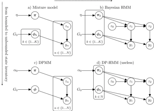
from b ounded to un b ounded state in ven tory GG G G G G G G G G G G G G G G G G G G G G G G G G G G G G G G G G G G G G G G G G G G G G G G G G G G G G GA GGGGGGGGGGGGGGGGGGGGGGGGGGGGGGGGGGGGGA
a) Mixture model b) Bayesian HMM
π φk η G0 zn yn k∈ {1...K} n∈ {1...N} πk φk η G0 z1 y1 z0 z2 y2 k∈ {1...K} c) DPMM d) DP-HMM (useless) π φ α0 G0 zn yn n∈ {1...N} πk φk α0 G0 z1 y1 z0 z2 y2 k∈N
Figure 2.1.1: Various clustering and HMM models
the nature of the observables,Ycould be a continuous space or a discrete space7. The
output distribution (overY) is denoted byF, and is parameterised byφ. Whenynis
discrete,Fcould be a categorical distribution (i.e. a multinomial distribution reduced
to one draw), andφa vector of probabilities. φis given a priorG0, in other words
the support ofG0is the parameter space forF.
In order for each statezto define a different emission probability,φis indexed by z.
We can now present the generative model for the Dirichlet mixture model, in figure 2.1.1a. It is further defined by:
cluster membership priorπ∼Symmetric Dirichlet(η) cluster membershipzn∼Categorical(π)
cluster parametersφk∼G0
observed datayn∼F(φzn)
(2.1.1)
G0 serves as a prior over the parametersφk of each cluster. Both the stateszn
and the cluster indexkare bounded for this model.
7For our part-of-speech tagging application,Yis the set of words, also cf. the notation introduced in section 2.2.3.
Recapitulating, we have: η∈R π∈RK zn, k∈ {1..K} yn ∈ Y (2.1.2)
Turning this model into an HMM means making then-plate Bayesian network a
dynamic Bayesian network (overt). Observed data now consists of sequences, each
of the formy1, ...yt, ...yT. We need to:
• define transition probability vectors (over destination states) for each origin state; thereforeπis now inside thek-plate
• replicate the state and emission nodes over time steps; while each emission node
ytis connected to a hidden state nodeztin the same way as before,
paramet-erised byφk, the hidden state is now parameterised by a transition distribution
which is indexed by the previous state, instead of being unique
This yields the HMM illustrated in figure 2.1.1b, with the following definitions: row of transition matrixπk∼Symmetric Dirichlet(η)
statezt∼Categorical(πzt−1) state parametersφk∼G0
observed datayt∼F(φzt)
(2.1.3)
Our graphical model represents the caseT = 2. We still have a finite state invent-ory, sok∈ {1..K}for this model, andzt∈ {1..K}. We assume that the initial state
z0is fixed. Rowsπk of the transition matrix are (vectors of) transition probabilities
for a given origin statek(the state corresponding to the row).t∈ {1...T}is the index
inside a given sequence (the data may consist of several sequences of different length, for simplicity we do not account for this in our notation here, and consider only one sequence).
How to make the state inventory unbounded, i.e. how to make the model non-parametric ?
Starting from the mixture model in figure 2.1.1a, a known construction to make the number of states unbounded is to turn the Dirichlet prior on the cluster identity into a Dirichlet process prior, yielding a DP mixture model (Antoniak, 1974). Now the number of statesKis unbounded,πis infinite-dimensional, andφkis defined for any
k∈N. The corresponding model is illustrated in figure 2.1.1c and defined as:
cluster membership priorπ∼SBC(α0)
cluster membershipzn ∼Categorical(π)
cluster parametersφk ∼G0
observed datayn ∼F(φzn)
(2.1.4)
SBC denotes the stick-breaking construction, which Ewens (1988) originally de-noted by GEM after the names of Griffiths, Engen and McCloskey. We do not detail the SBC further and refer to Teh et al. (2006) for details.
πis now an infinite-dimensional vector. Yet for any realisation of the model with
a finite number of data pointsN, only finite representations ofπwill be needed.
In the hope of obtaining an HMM model with unbounded states, we now apply the same changes to the HMM model in figure 2.1.1b, and obtain the model in figure 2.1.1d, which we might call the DP-HMM:
row of transition matrixπk∼SBC(α0)
statezt∼Categorical(πzt−1) state parametersφk∼G0
observed datayt∼F(φzt)
(2.1.5)
Upon closer inspection, however, we find that this model suffers from a fatal de-fect. For each origin statek, the DP prior indeed yields a new transition vectorπk
and a parameterφkfor the emission probabilityF. However, with probability 1, each
drawφk fromG0, since it is a continuous distribution8, will be different from any
previous drawφk0, k0 < k: almost surely, sampled states will not coincide. In other
words, with transition probabilities drawn independently, and no coupling between them, there is no reason for the chain to preferentially revisit already existing states. To apprehend the key issue, consider the following step of the stick-breaking con-struction of the DP:φk ∼ G0, i.e. for each draw from the DP, we need to sample
a new collectionφk from the base measureG0, with no guarantee that we will
en-counter already sampled states (again, unlessG0is discrete, because then the chances
could be non-zero, depending on the atom weights). To make sure we “recycle” states between source state distributions, we will make the base measure discrete: specific-ally, we will draw the base measure from another, higher-level DP, so that it is almost surely discrete.
In conclusion, while the DP is an interesting prior over clusters (for mixture mod-els), it is not helpful as a prior for state-to-state transitions.
π
kφ
kα
H
z
1y
1z
0z
Ty
Tβ
γ
k∈NFigure 2.1.2: Graphical model of the IHMM. Rowsπk, k ∈Nof the state transition
matrix are given a HDP prior. Cf. section 2.1.4 for a full description.
2.1.4
The HDP-HMM
To solve the issue of the DP-HMM, we must make sure we “recycle” states between source state distributions; to ensure this, we will make the base measure discrete: specifically, we will draw the base measureG0from another, higher-level DP, so that
G0is almost surely discrete. Beal et al. (2002) discussed this issue and proposed the
hierarchical Dirichlet process HMM (HDP-HMM) to solve it.
A note on nomenclature: in this thesis, we will use the terms IHMM and HDP-HMM interchangeably. The original “IHDP-HMM paper” Beal et al. (2002) derived the IHMM by taking limits when K → +∞, and proposed an inference scheme con-structed so that a parameter controls the propensity to create new states, and another parameter controls the probability of self-transitions. Later, Teh et al. (2006) (which uses the name “HDP-HMM”) proposed a Gibbs sampling inference scheme.
G0 is now a discrete distribution and transition probabilitiesπk are coupled, as
they are drawn from a DP with meanβ(in doing so, we assimilate vectors with the
categorical distribution they parameterise, e.g.βwith Categorical(β)).
We now formally define the HDP-HMM when applied to the task of part-of-speech tagging. We introduce the notation and terminology which we use in the remainder of this chapter. The resulting model is illustrated in figure 2.1.2.
Let a sentence of lengthTbe represented as a sequence of words (tokens, or
obser-vations in HMM terminology)y1, ...yt...yT, withyt∈ V, whereVis the vocabulary,
that is the set of observed words. We note card(V) =V, whereV is the total
num-ber of unique words. V is assumed to be fixed and known; at prediction (test) time,
In a generative view, tokens are generated from states (clusters)z1...zT according
top(yt|zt,φzt) = Categorical(yt|φzt), whereφsis the parameter for the emission probability for states;φs∈RV. In addition, we define dummy start and end states,
and corresponding start and end tokens, which enclose each sentence.
State transitions are governed by a state transition matrixπ, of which each row πkgoverns the transitions out of statek, so the probability of transitioning from state kat timetto statelat timet+ 1isp(zt+1 = l|zt =k) = πk,l. The total number
of states in usage for a given sample of the state sequences, including start and end states, is writtenK, soπT
k ∈RK andπ∈RK×K.
Thus far, our description corresponds to the structure of an HMM. We now place priors on πk andφz, so that the number of states is variable, and governed by a
hierarchical Dirichlet process. In addition, note that∀k,πkshould be of infinite size,
since the number of states is not bounded. At this point of the exposition, in order to prepare for writing out the MCMC procedure, which, to be implemented, requires manipulating finite structures, and to keep a mathematically correct notation, we will maintain the notation πk for the finite-dimensional vector, and denote byπk¯ the infinite-dimensional vector (equivalentlyπ¯ vs. π, andβ¯ vs. β, which will be
introduced below). Each sample ofπk uses only a finite number of states, since the
corresponding data uses only a finite number of tokens. Consequently, we will call the finite-dimensional vector a “collapsed” version of its infinite-dimensional coun-terpart; it is obtained by ignoring elements corresponding to unused states, i.e. one of the (countably infinitely many) states which are not represented in the data.
Theπ¯k, likeβ¯,behave like probability distributions, so they sum to one, and it
is essential to represent the probability mass which has been discarded in the pro-cess of collapsing (the “remaining mass”). For this reason, we append an extra ele-ment to each of the finite-dimensional counterparts:πk,K+1andβK+1are set so that
∀k,Pj=K+1
j=1 πk,j = 1and
Pj=K+1 j=1 βj= 1. ¯
πkis a sample from a Dirichlet process with concentration parameterαand base
measureβ¯shared by allπ¯k.β¯is also generated by a Dirichlet process, and is modelled by the stick-breaking construction (Sethuraman, 1994) with parameterγ, i.e. ∀i ∈
N,β¯i = ζiQj=ij=1−1(1−ζj)with∀k ∈ N, ζk iid∼ Beta(1, γ), which is also written ¯
β∼SBC(γ), cf equation 2.1.4.
The observation vectors also receive a prior, namely a symmetric Dirichlet distri-bution parameterised byH ∈R+.
Summing up, we have yt|zt,φzt ∼Categorical(φzt) zt|zt−1,πz¯ t−1 ∼Categorical(πz¯ t) ¯ πk|α,β¯iid∼ DP(α,β¯) ∀k∈N ¯ β|γ∼SBC(γ) φkiid∼ Dirichlet(H) ∀k∈N (2.1.6)
where we have denoted byHthe vector of sizeV with all elements set toH.
Note that there are two notation abuses in the lineπk¯ |α,β¯∼DP(α,β¯). The first is in DP(α,β¯): we really mean the DP which hasβ¯as its stick-weights sequence. The
second is in writingπk¯ |...∼DP(...):πk¯ is the stick-weights sequence obtained for the SBC for a draw from this DP; i.e. we completely ignore the positionsφk of the
point-masses (which are shared anyway), only to concentrate on the weights. We keep the hyperparametersα, γ andH fixed at all times (rather than giving
them priors or estimating them using maximum likelihood).
2.2
Distributed computing aspects
After describing and motivating the IHMM model, we now delve into the aspects related to distributed computing and software engineering. We chose to avoid custom (closed) computing clusters, as all prior work had done, but deliberately exploited widely available commodity computing power.
2.2.1
Commodity computing infrastructure
In terms of deployment platform, this research targets commodity computing clouds for impact, visibility, reproducibility, and reusability. In particular, we are interested in clouds which are pre-configured for distributed computing, such as (in 2009, when this research was undertaken) Amazon’s Elastic MapReduce (AEMR) platform, or Mi-crosoft Azure with MiMi-crosoft HTC or Dryad (Isard et al., 2007). These clouds in-tegrate storage, networking, computation, execution engine and language-level pro-gramming interface. The understanding of their economic model and advantages in 2009 is reflected in Armbrust et al. (2009).
At that time, distributed frameworks were in use in the industry and the open source community (Pig9, Hadoop (White, 2009), BigTable (Google proprietary (Chang
et al., 2006)) and HBase10, Hive (Thusoo et al., 2009), Cassandra (Lakshman and
9http://pig.apache.org/ 10http://hbase.apache.org/
Malik, 2010) ). In actual practice, in industry, they tended to be used mainly for non-statistical data manipulation: distributed grep’s, inverted indexing, hashing and searching, sort, distributed aggregation. Distributed machine learning was very much confined to research.
Yet such clouds bring several advantages for research in distributed machine learn-ing: they are publicly available, have a low upfront cost, use widely shared software configurations, and their hardware profiles are rather generic and reproducible. This summarises what we mean by “commodity” in this context, and is largely the opposite of custom computing clusters.
In particular, the requirement of reproducibility in computational sciences12has
gained traction in recent years. Tools, methods, supporting procedures by scientific publishers, research institutions, funding agencies were developed to address this need. For instance, reproducibility in research is one of the major drivers of the devel-opment of the Python notebook system Jupyter13, and it is indeed increasingly used to
document scientific methods in supplementary material14. Often, software
accompa-nying machine learning publications is available on Github. GitXiv was developed to coordinate the scientific preprint archive arXiv (largely used in the field of machine learning) with code repositories like Github and Bitbucket. Container technology such as Docker or Kubernetes, which was not widely available when this research was conducted, now allows even better archivability of the software configuration than what is achievable with commodity computing clouds.
The research focus on commodity cloud services proved to correctly anticipate fu-ture developments. AEMR, the deployment platform used in this research, was made public in April 2009, and was a forerunner in this area. It included a patched version of Apache Hadoop 0.18.3, a very early version. The Apache Hadoop Java open-source project15started around 2005 as a platform for map-reduce, and has since developed
in many other directions, to the point that it can nowadays be considered an ecosys-tem for distributed computing. Its latest stable version16at the time of this writing is
2.8.0, and was released on 22nd March 2017.
Hadoop fostered the development of Apache Mahout17, a Java package of
map-reduce implementations of popular machine learning algorithms, which became an Apache top-level project on 4th May 201018. The O’Reilly book “Mahout in Action”
11http://cassandra.apache.org/
12cf. Sandve et al. (2013) for a review of best practices, and Crick et al. (2015) for a suggested process 13earlier named IPython (Pérez and Granger, 2007)
14cf.https://github.com/ipython/ipython/wiki/A-gallery-of-interesting-IPython-Notebooks#
reproducible-academic-publicationsfor several examples of scientific publications with accompa-nying IPython (now Jupyter) notebooks and code.
15http://hadoop.apache.org/
16http://hadoop.apache.org/releases.html 17http://mahout.apache.org/
18https://blogs.apache.org/foundation/entry/the_apache_software_foundation_
(Owen et al., 2011), written by the original authors of Mahout, was published on 9th October 2011. Mahout still exists, and has changed drastically in the meantime, giving up the map-reduce dependency altogether (cf. section 2.4.2). Our project uses the Mahout linear algebra libraries, but not its implementations of algorithms.
The dates we have just cited demonstrate that this research exploited very novel technology. Indeed, the founding papers for applications of machine learning to mul-ticore platforms are arguably Dean and Ghemawat (2004) and Chu et al. (2007). To draw a parallel with technological developments at Microsoft, we can note that Mi-crosoft Dryad (Isard et al., 2007), a distributed execution platform based on more com-plex computational graphs than map-reduce, started as an internal research project in 2006; it had an academic release on 13th July 200919, including the Dryad platform
and DryadLINQ (Yu et al., 2008), which provided support to translate queries written in the LINQ query language into Dryad execution graphs. On 11th November 201320,
however Microsoft withdrew its support to Dryad, favouring Apache Hadoop instead. There now is a wide choice of managed distributed computing platforms, billed by compute time, from companies such as Databricks (Apache Spark), Google (Data-flow, Dataproc), Microsoft (Azure HDInsights running Apache Spark), Amazon Elastic MapReduce (now also running Apache Spark), Cloudera, MapR, Hortonworks.
Prior research in distributed probabilistic inference often did not target clouds or even private clusters or grids, but parallel multicore machines, sometimes running pseudo-distributed emulators. The few available deployments to clusters employed custom software. For instance, Nallapati et al. (2007) deployed on a cluster with 96 machines, using the PThread library and rsh for communication, Wolfe et al. (2008) ran a 32-machine cluster, (Doshi-Velez et al., 2009) deployed using Matlab Distributed Compute Engine. The research which comes closest to ours was (Wang et al., 2009), which used their own (Google Research) cluster with MapReduce, and compared with the Message Passing Interface (MPI), which is considered a standard for distributed computing in scientific fields which have a long tradition in high-performance com-puting such as climatology or theoretical chemistry), and is tailored less towards data partitioning and more towards computation partitioning. This shows that prior res-ults, to be reproduced, required an essentially identically configured and tuned setup. This section demonstrates the relevance, timeliness and significance, in the light of subsequent technological developments, of the research goal consisting of deploying on a commodity distributed computing cloud. In the rest of the present section 2.2, we detail the principles which guided our map-reduce development, as well as issues and best practices which emerged while implementing this research goal. We begin by recalling the basics of the map-reduce algorithm.
19https://www.microsoft.com/en-us/download/details.aspx?id=52604
2.2.2
Principle of map-reduce
We briefly outline the map-reduce algorithm21.Both mappers and reducers are functions which operate on key-value pairs, which we note < K, V > here. A mapper (ormap function) takes as input a single < K1, V1>pair, and outputs a single< K2, V2 >pair. A reducer (orreducefunction)
takes as input a list of< K2, V2>pairs with the same keyK2, which is equivalent to
defining their input as< K2, L2>whereL2stands for a list of values. The reducer
outputs a single< K3, V3>pair.
Here are the steps of the map-reduce algorithm:
Data preparation The input data is split up as< K1, V1>pairs, so that the data size
of< K1, V1>and computation needed by the mapper to process< K1, V1>
is orders of magnitude smaller than what can be processed on a mapper node.
< K1, V1>pairs are sent to mappers, which are distributed on slave nodes.
Map The map function is applied iteratively by each mapper to the< K1, V1>pairs
it has been assigned.
Shuffle < K2, V2 >mapper outputs are sorted over the entire cluster according
to keyK2, resulting in< K2, L2 >pairs. These pairs are then assigned to
reducers, which are also distributed on slave nodes. EachK2 is assigned to
exactly one reducer22.
Reduce The reduce function is applied iteratively by each reducer to the< K2, L2>
pairs it has been assigned. Each reducer may have several such pairs, and thus severalK2, to process.
Gather The reducer outputs are made available from the master node as a collection of< K3, V3>.
We now illustrate the procedure on the word-count algorithm: given as in-put a collection of text documents, it outin-puts a dictionary of unique words as-sociated to their count in the input corpus. Here, the mapper consumes <
document index,document>pairs and outputs< w,1>pairs (one for each wordw;
the number1here is nothing but a placeholder). These are shuffled, and reducers re-ceive the pairs corresponding to a single word, so that given< w, L >they only have