DEPARTMENT OF ECONOMICS
UNIVERSITY OF CYPRUS
QUALITY CONTROL FOR STRUCTURAL CREDIT RISK
MODELS
Elena Andreou and Eric Ghysels
Discussion Paper 2007-03
Quality Control for Structural Credit Risk Models
Elena Andreou
∗Eric Ghysels
†‡August 21, 2007
Abstract
Over the last four decades, a large number of structural models have been developed to estimate and price credit risk. The focus of the paper is on a neglected issue pertaining to fundamental shifts in the structural parameters governing default. We propose formal quality control procedures that allow risk managers to monitor fundamental shifts in the structural parameters of credit risk models. The procedures are sequential - hence apply in real time. The basic ingredients are the key processes used in credit risk analysis, such as most prominently the Merton distance to default process as well asfinancial returns. Moreover, while we propose different monitoring processes, we also show that one particular process is optimal in terms of minimal detection time of a break in the drift process and relates to the Radon-Nikodym derivative for a change of measure.
∗University of Cyprus, Department of Economics, P.O. Box 537, CY 1678 Nicosia, Cyprus, Phone:
+357 (22) 89 24 49, Fax: +357 (22) 89 24 32, E-mail: [email protected], Home page: http://www.econ.ucy.ac.cy/faculty/andreou/
†Corresponding author. Professor of Economics and Finance, Edward M. Bernstein Distinguished Professor of
Economics and Director of the Research Center for Financial Econometrics at the Kenan-Flagler Business School UNC, CIRANO and Department of Economics, Gardner Hall, CB 3305, University of North Carolina at Chapel Hill, Chapel Hill, NC 27599-3305, Phone: (919) 966-5325, Fax (919) 966-4986, E-mail: [email protected], Home page: http://www.unc.edu/ eghysels/
‡The authors would like to thank the editor and referees for their constructive comments. Elena Andreou would
like to acknowledgefinancial support of the University of Cyprus research grant number 8037-3312-32001 and the Leventis Foundation grant.
1
Introduction
One of the many areas Charles Nelson’s research touched is that on structural change, including the recent paper on structural breaks in the equity premium (Chang-Jin et al., 2005). This paper indirectly relates to this topic, in as far as expected returns (and potential breaks) are an input to structural credit risk models. Over the last four decades, a large number of structural models have been developed to estimate and price credit risk.1 The accuracy of credit risk models is essential for sound risk management and for supervisory evaluation of the vulnerability of lender institutions. In particular, the new capital adequacy framework (Basel II) encourages the active involvement of banks in measuring the likelihood of defaults.
The focus of the paper is on structural models of credit risk and the study of a neglected issue of structural breaks pertaining to such models. To set the stage, let usfirst review the key ingredients. The main ideas underlying many of the models go back to Black-Scholes (1973) and Merton (1974). Corporate liabilities (equity and debt) are viewed as contingent claims on the assets of thefirms. A
firm’s fixed liabilities constitute a barrier for the value of its assets. Then default is characterized as a boundary crossing problem. Namely, if assets drop below that barrier, the firm is unable to support its debt and therefore defaults.2 While conceptually simple, there are a lot of variations practitioners often use on the basic framework of Merton (1974) to assess credit risk. There arefive basic inputs: (1) a fundamental state variable, typically the market value of firm’s assets which is assumed to move randomly through time with a specified expected return and volatility, (2) debt, (3) interest rates, (4) a default boundary beneath and (5) a recovery ratio which postulates what debt holders receive in the event of default. Hence, to make the model operational we have to pick certain parameters, namely expected return - or drift in a diffusion setting and volatility -presumed constant in the Black-Scholes (BS) environment. The model produces a very commonly used measure, called distance to default (and an associated default probability).
It is a simplification to assume that structural parameters remain fixed. In fact, the expected return on assets clearly depend on the financial health of a firm. Moreover, while there is no obvious corporate finance theory underlying the Black-Scholes-Merton (BSM) type models it is clear from the few continuous time corporate finance models that managers ‘control’ the drift of asset returns, see e.g. Ou-Yang (2003) for a recent outstanding example. Structural shifts affect credit risk and this is the topic of our paper. When one examines distance to default in a BSM type model one realizes that there are two sources of variation in distance to default: (1) the random
1
For a review of structural credit risk models see for instance, Duffie and Singleton (2003), Eom, Helwege and Huang (2004), among others.
2
There are some nuances on this. For example in Merton’s model, afirm defaults if, at the time of servicing the debt, its assets are below its outstanding debt. A second approach, within the structural framework, was introduced by Black and Cox (1976). In this approach defaults occur as soon asfirm’s asset value falls below a certain threshold. In contrast to the Merton approach, default can occur at any time.
movements of the asset value, and (2) the potential shifts in the structural parameters. If one ignores parameter shifts then this may lead to biased inferences on credit default and investment misallocation decisions. It is the purpose of our analysis to design tests that monitor structural parameter variation.
To the best of our knowledge there are no formal procedures that allow risk managers to monitor for fundamental shifts in the structural parameters of credit risk models. Empirical evidence shows that there are structural breaks infinancial markets which affect fundamentalfinancial indicators such as, for instance,financial returns and volatility (e.g. Lamourex and Lastrapes, 1990, Andreou and Ghysels, 2006, Horvath et al., 2006), the shape of the option smile (Bates, 2000) and the equity premium (Pastor and Stambaugh, 2001, Chang-Jin et al., 2005). Our aim is to propose sequential methods for testing structural stability in credit risk models and default measures. This can be especially useful to risk managers and investment analysts in periods offinancial distress for monitoring in real-time the stability of corporations. The basic ingredients are the key processes used in credit risk analysis, such as most prominently the Merton distance to default process and obviously financial returns. In addition, the procedures we propose are easy to compute and therefore can be implemented on-line for potentially a large class of assets. Moreover, while we propose different monitoring processes, we also show that one particular process is ‘optimal’, using results of Moustakides (2004), where optimal refers to the minimal detection time of a break in the drift process. The optimal process relates to the Radon-Nikodym derivative for a change of measure. The optimality of the Radon-Nikodym derivative is rather fortunate, since it is a quantity very much familiar to risk managers, as it is so prominent in the option pricing literature - although its application will be in a new and different context here. Besides proposing various monitoring procedures and studying their theoretical properties, we also show via simulation that the proposed procedures have good finite sample behavior which can be used for the quality control of credit risk models. This is related to the broader issue of quality control in financial risk management (Andreou and Ghysels, 2006).
The rest of the paper is organized as follows. In section 2 we present BSM type structural models of credit risk and several extensions. In section 3 we introduce various monitoring processes and discuss their properties. Section 4 reports Monte Carlo simulation evidence on the performance of the various tests. The last section concludes the paper.
2
Structural Models: Merton and beyond
There are two broad approaches to describe afirm’s default process in the credit risk literature. The structural approach makes explicit assumptions about the dynamics of a firm’s assets, its capital structure and its debt and share holders. A firm defaults if its assets are insufficient according to
some measure/threshold. In the reduced form approach there is no relationship between default and say the firm value. Instead there is a less detailed information set (akin to that observed by the market) and dynamics of default are exogenously determined via a default rate or intensity by a jump process. Consequently in a structural credit risk model default is endogenously generated whereas it is exogenously given in a reduced form model. Moreover while reduced form models exogenously specify recovery rates, structural models determine recovery rates in terms of the value of the firm’s assets and liabilities at default. However the fundamental difference between these models is not in terms of the characterization of the default time but in terms of the information set available to the modeler. Moreover given that any structural model is only partially structural in the sense that it makes specific assumptions about certain attributes of the credit risk, the distinction between the structural and the reduced-form models can be thought of one of degree rather than existence. A further review of these approaches can be found in Duffie and Singleton (2003) and Eom et al (2004) inter alia. In the remainder of the paper we focus on so called structural models - yet our analysis of quality control could easily be extended to reduced form models.
The first structural model for assessing credit risk, typically of a corporation’s debt, dates back to Black and Scholes (1973) and Merton (1974). It is also sometimes called the BSM type model. A popular implementation of the model is the commercial KMV model used by Moody’s (Crosbie and Bohn, 2001) as well as academics (e.g. Vassalou and Xing, 2004).
Once a model is specified, its unknown parameters may be calibrated to observed data. The direct approach requires that one collects detailed information on an obligor’s balance sheet in order to estimate its fixed liabilities, which are generally assumed to be non-stochastic. The obligor’s capacity to carry these liabilities depends on the market value of its assets, which cannot be directly observed. However, by treating equity as a put option on underlying assets, one can use observed equity prices and volatility to recover the current value and volatility of the obligor’s assets.3 This procedure depends strongly on the assumed distribution for the asset return process. In practice, log-normality is nearly always imposed - since the basic foundations are the BS option pricing model. In this section, we present the original Merton model, based on log-normality, followed by a stochastic volatility extension based on the Heston (1993). Afirst subsection 2.1 is devoted to a short review of the Merton model. Subsection 2.2 introduces a class of monitoring processes that will play a key role in our analysis. Subsection 2.3 looks at extensions of the basic Merton model.
3
Practitioners sometimes also use an indirect approach, where one starts with agency ratings of the type issued by S&P and Moody’s. An obligor’s current rating is taken to be a sufficient statistic for some structural measure of its credit quality. In credit risk management applications, it is generally assumed thatfirms in the same rating grade share the same distance to default (defined later). By examining historical patterns of default for each rating grade, one can estimate unknown parameters of the return distribution process as well as the distance to default associated with each grade. In this paper we will rather assume that parameters are estimated directly, which is more closely related to the ‘econometric’ approach - the focus of our paper.
2.1
Default Probabilities and Distance to Default
The purpose of this subsection is to provide a brief review of the Merton (1974) model. It is assumed that the market value of the firm’s assets (VA(t)) follows a geometric Brownian motion
(GBM), dropping time indices for simplicity:
dVA=μVAVAdt+σVAVAdW (2.1)
where μVA is the expected return on VA(t) and σVA is the instantaneous volatility of VA(t) and
W(t) is a standard Wiener process. Furthermore, if we assume that the firm has only one class of debt that pays no coupon with face value F and maturityTM,the market value of the equity,
VE can be thought as a call option with maturity TM, strike price F and underlying asset VA(t).
Consequently the option pricing formula by Black and Scholes (1973) can be used to derive the value of the option i.e.
VE =VAN(d1)−F e−rTMN(d2)
where r is the risk-free rate of interest and N(.) is the cumulative standard normal distribution and d1 and d2 are the usual expressions derived for the BS model. Under the assumptions of the Merton model, Itô’s lemma yields the following relation between the volatility of equity value,σVE,
and the asset volatility,σVA,
σVE = VA VE ∂VE ∂VA σVA.
Since ∂VE/∂VA =N(d1) in the BS model, it follows for the Merton model that σVE =
VA
VE
N(d1)σVA. (2.2)
which is referred to in the literature as the optimal hedge equation.
Consequently the nonlinear equations (2.1) and (2.2) can be solved simultaneously in order to obtain values for the unobserved asset valueVA(t) and asset volatilityσVA using data on the equity value,
equity volatility, the risk-free rate, time to maturity and the strike price as inputs. Subsequently the distance to default (DD) can be calculated as (setting TM = 1):
DD= ln(VA/F) + (μVA− 1 2σ 2 VA) σVA (2.3) where default occurs if the face value of the debt exceeds the value of the assets. Intuitively the distance to default indicates how many standard deviations a firm is away from default given its net worth. We can think of the distance to default as a measure of an obligor’s leverage relative to the volatility of its asset values. As the value an obligor’s assets changes over time, its distance
to default changes as well. If assets fall below the value of fixed liabilities the distance to default drops below zero, and the obligor becomes insolvent. Given assumptions about the asset return process, an obligor’s distance to default is all that is needed to determine its default probability at a fixed horizon date.
2.2
Towards an optimal monitoring process: The Radon-Nikodym derivative
The above analysis assumes that there are no structural changes in (2.1) i.e. μVA and σVA aretime homogeneous. Given the empirical evidence of structural breaks infinancial markets and the motivation mentioned in the Introduction we assume that this maintained hypothesis is no longer valid. In monitoring changes in the parameters we shall focus, for the moment, on changes in the drift, i.e. μV
A since this determines expected returns.
In risk management applications real-time or sequential tests have the advantage that practitioners can apply these procedures on-line i.e. with the arrival of every new data observation. Sequential procedures require a historical startup sample which we will assume to run from1throughm.Then for all subsequent observations we are interested in testing the following null hypothesis:
H0:μVA(t) =μVA t=m+ 1, m+ 2, . . . (2.4)
where one builds on the so called non-contamination hypothesis (cfr. Chu et al., 1996) which assumes parameter constancy holds (thusμVA(t) =μVA fort =1, . . . , m) and one tests on-line. The procedures we propose to construct sequential tests will involve empirical processes, based on returns, volatility estimators and distance to default. However, the basic process of interest will be the Radon-Nikodym derivative (henceforth RND), which is a likelihood ratio, and will play a key role in testing. We will provide the details of the statistical theory in the next section. For the moment we focus on the population characteristics of the monitoring processes.
Under the alternative, we consider a single drift change,
H1:μVA(t) =
(
μVA(1) t=m+ 1, ..., τ > m
μVA(2) t=τ + 1, ..., n≤m+q (2.5) and we define the associated process:
α(t) = ( 0 t=m+ 1, ..., τ > m (μV A(2)−μVA(1))/σVA t=τ+ 1, ..., n≤m+q (2.6)
Hence, prior to some point t = τ : μ
VA(t) = μVA(1) and ∀ t > τ : μVA(t) = μVA(2). A change
prominently in option pricing since it is common to change probability measures (drifts that is). Since the Merton (1974) model is based on the BS model we go through these arguments to derive a process that will be used in our paper in an entirely new context.
In option pricing one denotes P as the natural or real-world probability measure and a different probability measureQwhich will be the risk-neutral probability measure - with the same volatility but different drift. In monitoring applications the two probability measures will be prior and post m,i.e.PnandPm.To establish the connection between the two probability measures one uses the Radon-Nikodym theorem. Let dPn/dPm be the RND. The Radon-Nikodym theorem tells us that
EPn(VA(n)|VA(m)) =EP m
(dPn/dPmVA(n)|VA(m))
Provided a boundedness (or Novikov) condition is satisfied, namely: EP[
Z n m
α(t)2dt]<∞ one has that:
dPn/dPm= exp [ Z n m α(t)dW(t)−.5 Z n m α(t)2dt] (2.7) for n≤ m+q. This RND will play a key role in the monitoring procedures we will study and in fact will have certain optimality properties discussed in the next section.
To conclude with BSM type models it is worth mentioning that there is a relationship between the above RND appearing in equation (2.7) and the distance to default process in equation (2.3). In particular, note that for any m < t≤m+q:
DD(t)−DD(m)−lnVA(t)−lnVA(m) σVA
=α(t) (2.8)
since the distance to default process is linked to the drift of the underlying asset process. The above equation shows that there are two sources of variation in distance to default: (1) the random movements of the asset value, and (2) the potential shifts in the structural parameters. Ignoring the possibility of parameter shifts may lead to faulty inference about default and it is the purpose of our analysis to design tests that monitor structural parameter variation.
2.3
The Merton model - stochastic volatility and other generalizations
A large literature emerged since the original work of Merton (1974). It is the purpose of this section to discuss how one can construct monitoring processes for a more general structural credit risk models and in particular stochastic volatility generalizations of the BSM model (Fouque et
al., 2006). We will show that, while RND’s are often readily available, though there remain some non-trivial practical implementation issues that emerge.
As a lead example, we will take a model which features stochastic volatility. Hence, the market value of thefirm’s assets (VA(t)) no longer follows a geometric Brownian motion (GBM). Instead,
following the example of Heston (1993), we assume that values of the asset follow the process: dVA(t) = μVAVA(t)dt+σVA(t)VA(t)dW1(t) dσ2V A(t) = (θ−κσ 2 VA(t))dt+ξσVA(t)dW2(t) cov(dW1(t), dW2(t)) = ρdt (2.9)
where σVA(t) is the time-varying instantaneous variance of the underlying asset, α/β is the
long-run mean of the instantaneous variance, β is the parameter that indicates mean-reversion of the variance, andξis the volatility of the variance process (or ‘volatility of volatility’). dW1anddW2are Wiener processes with correlationρ. The Heston model allows for volatility of the underlying asset to be randomly determined and assumes that it follows a mean-reverting (Ornstein-Uhlenbeck) process.
In the context of the above model the RDN for a shift in drift is specified in equation (2.7), assuming again the appropriate Novikov condition holds, with the α(t) process appearing in (2.6) replaced by: α(t) = ( 0 t= 1, ..., τ > m (μVA(2)−μVA(1))/σVA(t) t=τ + 1, ..., n≤m+q (2.10)
The above RND leads to several issues, which we discuss in the remainder of this section.
(A) Hidden State Variables
Similar to the option pricing context, the first observation emerging from equation (2.10) is that the RDN now involves the latent volatility process. Hence, as in prices of risk calculations (see e.g. Chernov and Ghysels (2000)) one has to extract hidden state variables in order to implement the monitoring processes. In this case the latent process is stochastic volatility. Obviously, there are many ‘filters’ to extract volatility. Hence the application of this will be based on some commonly used volatilityfilters. The case of stochastic volatility is only one example of hidden states.
(B) Distance to default
While the notion of distance to default is deeply rooted in structural models of credit risk, it is not easy to generalize to cases beyond the BS economy. For the case of stochastic volatility, distance to
default could potentially be backed out of corporate bond data (see Fouque et al. (2005) for further discussion), but this is rather involved. We will instead follow an approach often encountered in practice, which consists of obtaining the distance to default with the so-called plug-in estimators, i.e.: DD(t) = ln(VA(t)/F) + (μVA − 1 2σVA(t) 2) σVA(t) . (2.11)
Hence the Merton formula is used here with constant volatility being replaced by time-varying volatility - an approach similar to the popular BS implied volatility calculations. While the above is not a correct characterization of distance to default in a stochastic volatility economy, we will nevertheless use it as one potential monitoring process, mainly for comparing it with the BSM model.
Another advantage of the plug-in formula in equation (2.11) is that it can again easily be related to the RND with theα(t)process appearing in equation (2.10). In particular, note that for any m < t ≤m+q : DD(t)σVA(t)−DD(m)σVA(m)−(lnVA(t)−lnVA(m)) +.5(σVA(t) 2 −σVA(m) 2) σVA(t) =α(t) (2.12) where we notice again that we need the latent volatility process to characterize the mapping.
(C) Structural Breaks in State Variable Dynamics
So far, we focused exclusively on potential changes in the drift, and computed RND’s with regards to probability measures that were constrained by such changes. The stochastic volatility example, reveals that there might be more complex fundamental changes at stake. Indeed, the parameters that determine the volatility dynamics may also be subject to change and allowing for them would modify the RND. While we restrict our analysis, as far as RND characterizations is concerned, to shifts in the drift of returns, we will show by simulation, that the resulting processes do have power against changes in parameters pertaining to the volatility process. Obviously, the resulting monitoring procedures may no longer share some of the optimality properties in terms of minimal detection delay that will be discussed in the next section.
3
Empirical Monitoring Processes and Sequential Tests
In this section we discuss the change-point tests and the empirical series involved in monitoring diffusion models. First we present the general formulation of the problem and assumptions. Then we define the three alternative test statistics along with the asymptotic distribution of the sequential
statistics and their corresponding boundaries. We also discuss the optimal monitoring based on recent work of Moustakides (2004).
3.1
The general set-up
Assume that VA denotes the value of the assets of a firm which is distributed according to either
the BSM model in (2.1) or to the Heston model in (2.9). Given that the Heston model can be considered as a generalization of the BSM model and the empirical relevance of time-varying volatility, we develop the general set-up for sequential change-points in the context of the Heston specification. Note that other SV models can also be analyzed in our framework, which we will refer to below. The objective is to examine the null hypothesis that there is no structural change in the mean value of the assets. We assume that μV
A(t) over a historical sample of m observations is
stable,t= 1, ..., m,defined as the non-contamination sample which in addition allows the estimation of possible unknown parameters. Therefore the null hypothesis of testing on-line (that is with a sequential procedure updating as new data arrives) from t = m+ 1, m+ 2, ... is given by (2.4). Under the alternative hypothesis of a single drift change, at an unknown timeτ is given by (2.5). Denote a generic process by X(t) that we wish to monitor in order to test the hypothesis (2.4). Given the discrete data arrival as well as the specification of credit risk measures over discrete intervals (e.g. daily or monthly Distance to Default indicators in corporations) we treat, for monitoring purposes,X(t)as the discretely sampled observations from the continuous time models (2.1) and (2.9). In general,X(t) =h¡∆VA(t)/σVA(t)
¢
orh(∆DD(t))or RND-related processes for a measurable functionh(.)and ∆VA(t) = ln(∆VA(t))−ln(∆VA(t−1)).
For the Heston model under H0 we assume that X(t) (i) is a weakly stationary process with uniformly bounded(2 +δ)th moments for some 0< δ≤2 and (ii) is a strong mixing process such that
sup
A∈Fm
1 ,B∈Fm+n∞
|P(A∩B)−P(A)P(B)|≤n−ψ for all m, n≥1
whereFυdenotes theσ−field generated byXυ, Xυ+1, ..., X . Then lettingY(n) =X(1)+...+X(n), the limit σ2Y = limn→∞ n1EY(n)
2 exists, and if σ
Y > 0, then there exists a Wiener process {W(t),0≤t <∞}such thatY(n)−σW(n)a.s.= O(n1/2−ε)whereε=δ/600(see for instance, Philip
and Stout, 1975, Theorem 8.1, p.96). This theorem is general enough to cover many applications. Under the above mixing and stationarity conditions X(t)satisfies the strong invariance principle:
X
1≤t≤n(X(t)−E(X(t)))−σXW(n) a.s.
= o(nγ). (3.13) with some 0 < γ <0.5 and W(.) a Wiener process. Hence (3.13) holds under H0. Consequently,
under the null,X(t)satisfies the Functional Central Limit Theorem (FCLT) Y(n) :=T−1/2X
1≤t≤n(X(t)−E(X(t)))→σXW(n). (3.14)
The above conditions are satisfied by the Heston model and other stochastic volatility models (SV). Genon-Catalot et al. (2000, Proposition 3.2, page 1067) show that the processσVA(t)in the Heston
model isβ−mixing (which impliesα−mixing). The key insight of Genon-Catalot et al. (2000) is that continuous time SV models can be treated as hidden Markov processes when observed discretely which thereby inherits the ergodicity and mixing properties of the hidden chain. Carrasco and Chen (2002) extend this result to generalized hidden Markov chains and show β−mixing for the SV-AR(1) model as well as a family of GARCH models. Other SV specifications found in Chernov et al. (2003) also satisfy the β−mixing condition. Hence, using the continuous mapping theorem, for the SV model in (2.9) and any continuous measurable function h(.) the monitoring processes X(t) = h(∆VA(t)) and X(t) = h(∆DD(t)), which are functions of σVA(t), are also β−mixing.
For instance, in the Heston model the FCLT holds if X(t) = ∆VA(t) or (∆VA(t))2 are strongly
mixing and have finite (4 +δ)th moments. Necessary and sufficient conditions for the existence of moments in SV models can be found for instance in Chernov et al. (2003) that deal with moment based estimation of these models.
For completeness we note that the BSM model is the simplest form of diffusion for which ∆VA(t)
is an independent and identically distributed (i.i.d.) process and the CLT applies. Hence for the BSM model, under H0,∆DD(t) is also an i.i.d. process (since it is a linear function of∆VA(t)).
3.2
Sequential change-point statistics
The following sequential test statistics, Sn, for monitoring the process Xt are considered: The
Fluctuation (FL) detector: SnF L= (n−m)σ0−1(Xn−m−Xm), (3.15) where Xn−m= 1 n−m Xn j=m+1Xj
measures the updated mean estimate,Xn−m, from the historical mean estimate,Xm.
The Partial Sums (PS) statistic:
SnP S =Xm+k
i=m+1(Xi−Xm), k≥1 (3.16) is similar to the Cumulative Sums (CUSUM) test of Brown et al. (1975) in that it monitors the
least squares residuals Xi−Xm.
The Page (PG) CUSUM statistic is:
SnP G=Xn
i=1Xi−1min≤i<n
Xn
i=1Xi (3.17)
which can also be considered as a Partial Sums type test since for an independentXi,it is equivalent
toPni=1Xi−Pin=1−rXi for anyr, 1≤r ≤n(see Page, 1954).
The asymptotic distribution of the FL and PS statistics can be found in Horvath et al. (2006) under the conditions discussed in the previous section and for a general boundary function. Given that the PG test can be written in terms of partial sums the FCLT also applies to this test.
The FCLT for the above sequential test statistics holds if we replace the asymptotic variance in (3.14) of dependent processes σX = P∞t=−∞cov(Xt, X0) by a consistent estimator. There is a large literature on alternative Heteroskedastic and Autocorrelation Consistent (HAC) estimators. What is important to emphasize is that the asymptotic variance is based on an estimator of the uncontaminated samplem.4
3.3
Empirical Monitoring Processes
Given the above test statistics we use the following monitoring processes: (i) The observed processes for the standardized changes in the value of the assets,∆VA(t)/σVA(t), and the changes in Distance
to Default, ∆DD(t), (ii) The Radon-Nikodym derivative given by (2.7) where α(t) is based on the estimated parameters and more precisely on the standardized difference of mean value of
∆VA(t)estimates during the monitoring and historical periods,
¡ b
μVA(n−m)−μbVA(m)¢/σVA such
as ¡∆VA(n−m)−∆VA(m)
¢
/σVA,and (iii) The Radon-Nikodym derivative given by (2.7) where
α(t) are the observed processes in (i) i.e. ∆VA(t)/σVA and ∆DD(t).
Given the above two structural models, σVA(t) = σVA in the BSM model, whereas in the Heston
model the stochastic nature ofσVA(t)is based on dynamic volatilityfilters with parameters obtained
over the historical sample m.Nevertheless, for the Heston model we also consider the misspecified historical volatility estimators, mainly for comparison purposes with the BSM model. It is also acknowledged that instabilities in the Heston model could be due to the SV parameters for which we specify other types of monitoring processes that yield more power in detecting breaks in volatility such as functions of ∆VA(t)/σVA(t) and ∆DD(t) that approximate the quadratic behavior of the
process, ¡∆VA(t)/σVA(t)
¢2
and (∆DD(t))2.
4Horvath et al (2006) provide some promising simulation results of updating sequentially the HAC estimation for
3.4
Optimal Monitoring Schemes
There are various optimal schemes and criteria. Let the true break point be τ , and suppose the estimated breakpoint is denoted byˆτ and is determined by:
ˆ τ = inf
t≥mS(t)> b(t) (3.18)
then if we define the expected detection delay asE[ˆτ−τ], we are interested in the minimization of the average detection delay or the average run length (ARL). Lorden (1971) introduced an expected delay min—max criterion and established the asymptotic optimality of the CUSUM test under the proposed min-max criterion.
Given the topic of the paper we are more interested in the optimality results of detecting changes in continuous time processes. Most of the attention has focused on a Brownian motion with drift. This means that when VA(t) follows a geometric Brownian motion (GBM), we can consider the
case of ∆VA/σVA,which is a drifted BM. The optimality of CUSUM has been established for the
BM with constant drift by Beibel (1996), Ritov (1990) and Shiryayev (1996). Moustakides (2004) established the optimality of the Page (1954) CUSUM test in detecting changes in the statistics of Itô processes, in a Lorden-like sense, when the expected delay is replaced in the criterion by the corresponding Kullback—Leibler (K—L) divergence. However, in the case of the drifted BM, both the Lorden expected delay and K-L divergence criteria coincide, which means that for monitoring drift parameters in BSM type models, the Page CUSUM test is an optimal test both in terms of expected delay and K-L divergence criteria. Therefore, we consider again the log likelihood ratio, which according to equation (2.7) equals:
un≡logdPn/dPm = [ Z n m α(t)dW(t)−.5 Z n m α(t)2dt] (3.19) Then Moustakides (2004) shows that the Page CUSUM test:
S(n) =un− inf
0≤t≤nut (3.20)
is optimal which implies that using the RND in a Page CUSUM test yields the optimal monitoring process and test statistic combination.
Some important caveats apply, however. Let us consider again the BS GBM and assume as in equation (2.5) that there is a single drift change. To show optimality, Moustakides (2004) assumes that the GBM before and after the break are known.5 Hence, there is no parameter estimation
5Moustakides (2004) also imposes other regularity conditions, which are standard, such the Novikov condition to
uncertainty and therefore μVA(1), μVA(2) and σVA are known a priori, what is not known is the
timing of the breakpointτ .Obviously, we do not know the parameters in practice, which introduces estimation uncertainty. It also explains why we need to consider different versions of the RND which rely on different estimators of the drift parameters. It is in part the purpose of the simulation section to assess how estimation uncertainty affects the optimality properties of the Page CUSUM test with the RND as monitoring process. Whether the Page test yields the lowest ARL even in the presence of estimation error is examined via simulations. This is the topic to which we return in section 4. An attempt to extend the Moustakides (2004) results to the Heston model is faced by the critical role of the likelihood ratio representation of the Page test in deriving the optimality results. For the Heston model as well as other SV models, mentioned above, the likelihood function is not computationally tractable. Even if we consider the hidden Markov representation of SV models (Genon-Catalot et al., 2000) in relation the results in Fuh (2003) for the optimality of the CUSUM for hidden Markov chains, then the problem remains that the likelihood function is not computationally tractable except if we use numerical integration methods. While simulation-based likelihood methods could potentially be considered to compute the RND and extract the hidden state variables, they would be computationally intensive to implement especially in a sequential framework. We want to keep the sequential monitoring processes simple and easy to apply and therefore resort to empirical processes that are not computationally involved.
It is also worth noting that recent extensions of structural credit risk models involve structural parameters that are state/regime dependent where the state could be the phase of the business cycle or thefirm’s external rating (e.g. Bangia et al., 2003). For instance cash-flows and bankruptcy costs may be state-dependent. The testing procedure proposed here can be extended to capture changes in the regime switching mechanism. This extension would imply that some of the RN related processes would of course differ from the standard diffusion credit risk models. Such extensions as well as an investigation of the optimality properties of the Page test and RN related processes for such models is left for future work.
3.5
Boundaries
The monitoring scheme is a stopping time, determined by a statistic,Sn, and a thresholdb(m, n),
according to τg(Sn) ≡ min{n ≥ m, Sn ≥ b(m, n)}. The theory of the drifted Wiener process
provides a way to find the appropriate boundaries. Linear and parabolic boundary functions can be considered that grow with the sample size at approximately rates p(n/m) and plog(n/m), respectively. For i.i.d. processes Robbins (1970) suggests the boundary
and Seigmund (1985) shows the optimality of this boundary for independent processes and simple hypotheses. We apply this boundary to the sequential tests of the BSM monitoring processes. Chu et al. (1996) extend the i.i.d. results of Robbins and Seigmund (1970) to monitoring procedures where the partial sum of the residuals and recursive estimates in linear time series obey the FCLT, under milder restrictions on general class of boundary functions (see Theorem 3.4, p. 1051 and Theorem A, Appendix A, p. 1062). The following boundary is derived analytically for the sequential CUSUM-type and Fluctuation tests:
b2(n/m) = µ (n/m)(n/m−1) ∙ α2+ ln µ n/m n/m−1 ¶¸¶0.5 (3.22)
whereα2 = 7.78and 6.25 gives the 95% and 90% monitoring boundaries, respectively. In addition, Leisch et al. (2000) specify the boundaryb3(t) =λ
p
2 log+(n/m)wherelog+(n/m) = 1if(n/m)≤e and log+(n/m) = log(n/m) if (n/m) > e, for which the critical values λ for the increments of a Brownian bridge are obtained via simulations in the context of Generalized Fluctuation tests (see for instance, Table 1, p. 846, Leisch et al., 2000). Zeileis et al. (2005) argue that simulation evidence forλplog+(n/m) suggests that most of the size of the test is used at the point where the boundary changes from being constant to growing and this makes it inappropriate for a process with growing variance such as the Brownian bridge. Hence they suggest a simple boundary that has the advantage of not using up the size of the corresponding test at the beginning of the monitoring period while at the same time growing in a linear manner given by
b4(n/m) =λ·(n/m) (3.23)
where λ is the simulated critical value for alternative monitoring horizons (shown in Table III in Zeileis et al., 2005). In the remainder of the analysis we consider b2(n/m) and b4(n/m) and note that these linear boundaries have an intersection point during the monitoring period. For instance, if the historical sample isnthenb2(n/m) andb4(n/m)intersect at2mfor a 10% significance level. After the intersection point the slope ofb4(n/m) is lower than that ofb2(n/m) which implies that it is more likely to capture small breaks late in the sample. In contrast, before the crossing point b4(n/m) rests higher then b2(n/m) which means that the probability to detect an early break is lower for b4(n/m) relative to b2(n/m). We apply b2(n/m) and b4(n/m) to the sequential tests of the Heston monitoring processes.
The choice of the boundary in sequential testing is traditionally followed based on the minimization of the ARL which we address in the simulation analysis. In turn the detection delay also depends on the choice of the historical samplem which we also address via simulations.
4
Simulation Analysis
In this section we examine the properties of the sequential change-point tests defined in section 3.2 for the alternative monitoring processes presented in section 3.3 for the BSM and Heston models. The first subsection describes the Monte Carlo design and the second subsection discusses the simulation results.
4.1
The Monte Carlo Design
We simulate two structural models for the value of the assetsVA using discretization of the BSM
and Heston parameterizations. First consider the Euler discretization of BSM in (2.1):
∆VA=μVAVA∆t+σVAVA √
∆tε
where the discretized Wiener process is√∆tε,whereεis a standard normal random variable. This discretization yields the following simulation process forVA,t+∆t.Since ∆VA:=VA,t+∆t−VA,t,
VA(t+∆t) =VA(t) +μVAVA(t)∆t+σVAVA(t) √
∆tε. (4.24)
In practice it is usually more accurate to simulate lnVAthanVA.From Ito’s lemma (2.1) yields:
dlnVA= (μVA −0.5σ 2 VA)dt+σVAdW so that VA(t+∆t) =VA(t) exp h (μVA −0.5σ2VA)∆t+σVA √ ∆tεi (4.25)
Note that although (4.24) is only true in the limit as ∆t → 0, equation (4.25) is exactly true for all ∆t. For simplicity we set∆t= 1 in the simulations. Given that Distance to Default is defined in (2.3) we use the simulated processes (4.25) to obtain the simulated path forDD and setF as a constant assumed to be 61%, 50% and 20% of the sample mean forVA.These values were obtained
from the descriptive statistics of the sample of US banks in the database of Andreou et al. (2006) and correspond to the sample mean, 25th, 5th and 1st percentile of the sample values of F for these banks, respectively. From the same database we obtain sample averages which we use for the starting values ofVA(0), σVA(0),and μVA(0).
6
Similarly the Euler discretized Heston model is: VA(t + ∆t) = VA(t) + μVAVA(t)∆t +
VA(t)σVA(t) √ ∆tε1 and σ2VA(t+∆t) = σ 2 VA(t) + (θ−κσVA(t))∆t+ξσVA(t) √
∆tε2 where the two correlated standard normal processes ε1 and ε2 are given byε1 =x1 and ε2 =ρx1+ (1−ρ2)0.5x2
wherex1 and x2 are univariate independent standard normal processes. For simplicity we assume ρ= 0.Note that this assumption also simplifies the specification of the RND for the Heston model and makes it more comparable to the BSM model. There is a large literature on the appropriate simulation schemes of stochastic volatility models. Although a comparison of these methods is beyond the scope of the present paper we have used the Milstein correction for simulating the Heston model (Kloeden and Platen, 1995):
VA(t+∆t) =VA(t)[1 +μVA∆t+σVA(t)ε1+ 0.5σ 2 VA(t)(ε 2 1−∆t)] σ2V A(t+∆t) =σ 2 VA(t) + (θ−κσ 2 VA(t))∆t+ξσVA(t)ε2+ 0.25ξ 2(ε2 2−∆t) (4.26)
In the Heston model we apply the same values as in the BSM mentioned above. For the parameter values in (4.26) we consider those in the estimated model of Andersen et al. (2002) such that θ= 0.0074, κ= 0.0123, ξ = 0.0578, ρ= 0(in Table VI, column 7, p. 40).
The above models refer to the simulated processes under the null hypothesis of parameter stability. Under the alternative hypothesis we consider a permanent mean shift in the drift of the two models in order to assess the power of the sequential monitoring procedures. For the Heston model we also consider the alternative hypothesis of changes in the SV parameters. Details of the sizes and the time of the break as well as the non-contamination sample sizes are discussed in the next section. For each model we obtain the simulated returns process∆VA and define the empirical monitoring
processes discussed in section 3.3 and their corresponding test statistics in section 3.2, namely the Fluctuation (FL), the Partial Sums (PS) and Page (PG), (3.15), (3.16) and (3.17), respectively. We evaluate the test statistics using the boundaries defined in section 3.5. For the BSM model we use the linear Robbins boundary defined in (3.21) given we are dealing with an i.i.d. process and for the Heston model we use the parabolic Chu et al. and linear Zeileis et al. boundaries in (3.22) and (3.23), respectively. The tests are evaluated in terms of their size and power properties and in terms of their detection delay measured by the Average Run Length (ARL). We report these criteria mainly for conciseness purposes. 7
4.2
Simulation results
The simulation results for the BSM model found in Tables 1 and 2 present the size and power properties, respectively, of the three alternative statistics, the Fluctuation (FL), the Partial Sums (PS) and Page (PG), (3.15), (3.16) and (3.17), for the five monitoring processes: The first row corresponds to the RND for the standardized estimated mean drift parameters
¡
∆VAn−m−∆VAm
¢
/σVA which can also be considered as the Maximum Likelihood estimates in a
7
Additional criteria such as Maximal Run Length (MRL) that refers to the maximal detection delay, the standard deviation of thefirst hitting time and the distribution of thefirst hitting time can also be obtained from the authors.
geometric Brownian motion model. We denote this processRN−M L in the Table 1. The second row refers to the monitoring process of standardized returns ∆VA(t)/σVA, and the third to its
corresponding RND denoted byRN−∆VA(t)/σVA. The fourth row refers to the changes in Distance
to Default, ∆DD(t) monitoring process and its RND equivalent denoted byRN−∆DD(t). It is worth noting that Moustakides (2004) sets σVA = 1 in the BSM model whereas in the simulation
design we consider σVA 6= 1 which is estimated based on the historical sample variance estimator
from the noncontamination sample of m observations. Since the properties of the boundary functions depend on m we consider historical sample sizes, m = 125,500 observations and set the monitoring horizon q = 2m,3m,4m. Under the null hypothesis, H0 : μVA(t) = μVA, and as
expected when q → ∞ the size of the test improves which is shown by the results in Table 1 for q = 4m as opposed to 2m.8 Moreover we find that as m increases the size of all tests improves. Overall the results show that for q= 4mand different m,the Page test yields simulated size close to the 5% nominal size for four out of the five monitoring processes, as opposed to the FL and PS tests that appear slightly more conservative in terms of size.
We now turn to evaluate the properties of the sequential monitoring methods under the alternative hypothesis of a structural change inμVA of break sizesδm such thatH1:δmμVA fort=m+τ+ 1, ...
whereδm = 2,2.5,3,4and μVA is the parameter under theH0,at change-point locationτ = 1.1m
where m = 125,500 and the monitoring horizon is q = 4m. In Table 2 we evaluate the aforementioned test statistics and monitoring processes in terms of their power (measured as the mean number of rejections under the alternative) to detect a break and in terms of their detection delay measured by the ARL. As expected wefind that as the size of the break increases the power of the tests improves and the detection delay is minimized. This result holds for all tests, monitoring processes and historical samples sizes,m. Out of the three tests the Page (PG) test appears to have the highest power and lower ARL. We also compare the alternative monitoring processes and find that the Radon-Nikodym derivative based on ∆VA(t)/σVA, denoted byRN −∆VA(t)/σVA, yields
the optimal monitoring process in terms of the lowest ARL - as indicated by the ARLs with a (*) sign. Moreover, this is the monitoring process with the relatively highest power. In almost all cases, the two monitoring processes,RN−M Land∆VA(t)/σVA, give the same ARL andRN−M Lyields
only slightly higher power than∆VA(t)/σVA.One explanation why theRN−M Lyields lower ARL
thanRN−∆VA(t)/σVA is that infinite samples the estimation error of the the mean driftμVA (and
variance parameter σVA), affects the ARL. As the size of the break, δm, increases the deviation
between the ARLs of these two processes, RN −M L and RN −∆VA(t)/σVA, increases. Finally,
the monitoring processes that relate to the Distance to Default industry standard, ∆DD(t) and RN−DD(t),have good power and similar ARLs toRN−∆VA(t)/σVA andRN−M Lespecially
for large break sizes δm <3.9
8
Note that the examination of thefinite sample properties of these tests requires monitoring horizons which are equal to empirically relevant samples, hence our choice ofq.
9
Summarizing the BSM model simulation results show that the Page test has empirical size close to the nominal one when using the Robbins boundary, b1(t) and yields the highest power and lower ARL compared to the Partial Sums (PS) and Fluctuation (FL) tests for all break sizes (δm) and
historical samples, m. In addition, across the different monitoring processes we find that the one based on the RND which involves the standardized asset value growth rate, RN −∆VA(t)/σVA,
yields the optimal monitoring process in terms of the lowest ARL for all three tests, break sizes and historical samples.
Turning to the Heston model simulation results we examine the monitoring processes mentioned above augmented by the estimation of σVA(t). We employ two widely used discrete volatility
estimators (given the discrete nature of our monitoring schemes) such as the GARCH model and RiskMetrics (RM) industry standard. We contrast these estimators with the misspecified constant historical variance estimator (denoted by CVOL in Table 3) mainly for comparison purposes with the BSM model and with the approach used by practitioners based on the implied volatility of option prices. Table 3 presents the size of the three sequential change-point tests for the Chu et al. parabolic and the Zeileis et al. linear boundaries, in (3.22) and (3.23), respectively. We report the results for only two monitoring processes that yield good size and power results, ∆VA(t)/σVA(t)
in the upper part of Table 3 and the standardized estimated change in the drift parameters
¡ b
μVA(n−m)−μbVA(m)¢/σVA (in the lower part of this table). We find that the drift estimators
proposed by Merton (1980) based on the difference in the returns over long spans yields an improved performance of these tests, as shown in the lower part of Table 3. However, this process is oversized compared to∆VA(t)/σVA(t) and for the linear boundary size is closer to the 5% nominal one for all
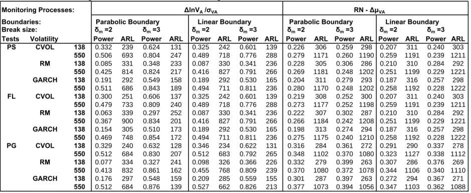
statistics and monitoring processes. The power of these processes for the Heston model is examined in Table 4 under the alternative of a break in the mean of VA(t) (as discussed above for the BSM
model).10 Interestingly we find that monitoring the observed standardized ∆VA(t)/σVA process
yields higher power and lower ARLs. One possible explanation is that it is very difficult to estimate the mean of diffusions (also argued in Merton, (1980)) especially in the presence of SV. Moreover we find that the GARCH and RM scaling estimators for ∆VA(t) yield slightly better power than
the constant historical volatility but overall the power improves as the historical samplemincreases and for relatively large breaks. Overall the ARLs obtained from monitoring breaks in the mean of VA(t)that follows a Heston model are higher than the ARLs obtained from monitoring a BSM.
This result is not surprising given that the dependence as well as the nonlinearity in the SV model. Note that monitoring the industry standard of the scaled differences in the Distance to Default yields good size but very weak power under the Heston model (and hence for conciseness we do not report it in the Tables). Two explanations for this result are the fact that the traditional Merton Distance to Default measure with plug-in estimates in (2.11) is not the appropriate specification
for logarithmic boundaries. However, we focus on the Robbins boundary due to its optimal properties mentioned in section 3.5.
1 0
in the presence of the SV and that DD(t) is not a good approximation of changes in the drift of a diffusion.
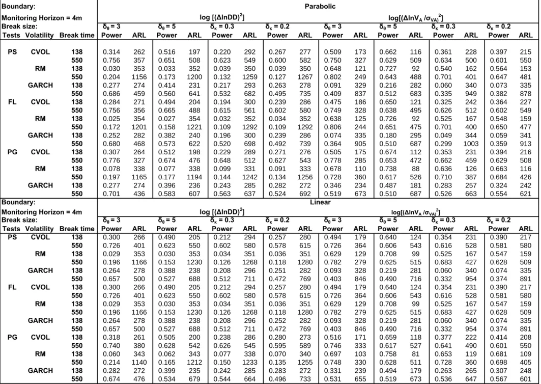
We further apply our methods to examine the instability of the Heston model due to structural changes in the SV parameters. We consider two simple alternative hypotheses of permanent increases in the volatility parameters θ and κ given by H1 : δθθ where δθ = 3,5 and H1 : δκκ
where δκ = 0.2,0.3 (where under the H0 :δθ = 1 and δκ = 1) atτ = 1.1m. Given that the FCLT
conditions are satisfied by the nonlinear functions¡∆VA(t)/σVA(t)
¢2
and(∆DD(t))2we examine the properties of sequential change-point tests based on monitoring these quadratic transformations. Table 5 reports the size results where we observe that the Page (PG) test appears to be oversized when used in relation to the Riskmetrics (RM) estimator. The power of these tests is presented in Table 6 which shows that the GARCH and historical volatility estimator (CVOL) have good power for detecting breaks in the volatility parameters whereas the RM appears to have poor power for monitoring(∆DD(t))2. Overall the power and ARLs as expected are improved for the parabolic as opposed to the linear boundary. However despite the fact that we are dealing with an early break in the sample the ARLs of the power of the two boundaries is quite close.
Summarizing the Heston model simulation results show that the monitoring processes
∆VA(t)/σVA(t)and
¡
∆VA(t)/σVA(t)
¢2
have good size and relatively higher power and lower ARL for detecting breaks in the mean and volatility, respectively. This result holds for all three sequential change-point tests, for any volatilityfilter and any historical sample,m. Again the Page test yields the highest power and lowest ARL relative to the Fluctuation and Partial Sums tests.
Last but not least, we have found that the above results are robust to: (i) other HAC estimators i.e. the Quadratic Spectral HAC estimator with prewhitening, (ii) other break dates suchτ = 1.5mand 2m and break sizes as well as gradual and multiple structural changes that may also affect credit risk (e.g. Bangia et al., 2002), (iii) other historical sample sizes m = 250,750,1000, (iv) other parameters for the Heston model for ρ = 0 such as θ = 0.0025, κ = 0.0063, ξ = 0.0229, ρ = 0 found in the estimation results in Andersen et al. (2002) (Table III, column 7, p. 37) and ρ=−0.3799, θ= 0.0107, κ= 0.0162, ξ = 0.0771also found in Andersen et al. (Table VI, column 8, p.40) and finally other starting values.
5
Conclusions
The focus of the paper is on structural models of credit risk. A common assumption in these models is that their parameters remain invariant through time. Yet, in practice these parameters are subject to change. We study the issue of fundamental shifts in the structural parameters of credit risk models and provide sequential test procedures that are relatively easy to implement.
We propose different monitoring methods and processes and address their optimality in terms of minimal detection delay of a break. The simulation analysis shows that these monitoring methods have good properties which suggest that they can be used as formal quality control procedures that can allow risk managers to monitor shifts in the structural parameters of credit risk models. The paper presents various tests to monitor changes in the parameters of discretely sampled diffusions and extends and in particular makes operational, the optimal sequential schemes of Moustakides (2004). From a practical point of view, the procedures we suggest have the appealing feature that they involve processes that are very familiar to practitioners. In particular, the optimal process based on the Radon-Nikodym derivative is rather fortunate, since it is a common and well understood concept in the risk management literature, although it is typically applied in a different context, namely not a statistical context but rather to compute a change of measure between objective and risk neutral probability measures.
Our analysis focuses on structural credit risk models. Yet, the quality control tools we present can be applied to a larger class of credit risk models. For example, sequential tests can be applied to test the parameter stability of reduced form models. It would not be clear a priori what would be the optimal monitoring process, a topic which would need further exploration. Likewise, one of the most popular approaches to bond risk measurement in practice is direct credit spread modeling. The Merton framework suggests that credit spreads should vary with equity volatility, as extensively explored in Campbell and Taksler (2003). It is interesting to note that the Campbell and Taksler paper is in fact implicitly based on a structural break argument, namely they rely on the Campbell, Lettau, Malkiel and Xu (2001) paper which shows that idiosyncratic volatility has fundamentally changed over the last 20 years or so. One could again investigate how to monitor for structural breaks in the context of such credit spread models.
References
Andersen T. G., L. Benzoni and J. Lund (2002), An empirical investigation of continuous-time models for equity returns, Journal of Finance 57, 1239-1284.
Andrews D.W.K. and J. Monahan, 1992. An improved heteroskedasticity and autocorrelation consistent covariance matrix estimator. Econometrica, 60, 953-966.
Andreou, E. and E. Ghysels (2006), Monitoring for Disruptions in Financial Markets, Journal of
Econometrics, 135, 77-124.
Andreou E., Bartram S. and E. Ghysels (2006), Real-time Monitoring of International Bank Insolvency Risk, Working Paper.
Bangia A., F.X. Diebold, A. Kronimus, C. Schagen and T. Schuermann (2002), Ratings Migration and the Business Cycle, with Applications to Credit Portfolio Stress Testing, Journal of Banking
Bates D.J. (2000), Post-’87 crash fears in the S&P500 futures option market, Journal of
Econometrics, 94, 181-238.
Beibel, M. (1996), A note on Ritov’s Bayes approach to the minmax property of the CUSUM procedure, Annals of Statistics,24, 1804—1812.
Black, F., and J. C. Cox (1976), Valuing Corporate Securities: Some Effects of Bond Indenture Provisions,Journal of Finance, 31, 351-367.
Black, F., and M. Scholes (1973), The pricing of options and corporate liabilities,Journal of Political
Economy, 81, 637-659.
Brown R.L., J. Durbin and J. M. Evans (1975), Techniques for testing the constancy of regression relationships over time, Journal of the Royal Statistical Society, Series B, 37, 149-192.
Campbell J. and G. B. Taksler (2003), Equity Volatility and Corporate Bond Yields, Journal of
Finance, 58, 2321-2349.
Campbell J., M. Lettau, B. Malkiel and Y. Xu (2001), Have Individual Stocks Become More Volatile? An Empirical Exploration of Idiosyncratic Risk, Journal of Finance 56, 1-43.
Carrasco M. and X. Chen (2002), Mixing and moment properties of various GARCH and Stochastic Volatility models,Econometric Theory, 18, 17-39.
Chang-Jin, K. Morley, J.C. and C. R. Nelson (2005), The Structural Break in the Equity Premium,
Journal of Business and Economic Statistics, 23, 181-191.
Chernov, M. and E. Ghysels (2000), A Study Towards a Unified Approach to the Joint Estimation of Objective and Risk Neutral Measures for the Purpose of Options Valuation,Journal of Financial
Economics, 56, 407-458.
Chernov M., A.R. Gallant, E. Ghysels and G. Tauchen (2003), Alternative models for stock price dynamics, Journal of Econometrics, 116, 225-257.
Chu C.S.J., Stinchcombe M. and H. White (1996), Monitoring structural change, Econometrica, 64, 1045-1065.
Crosbie, P.J. and Bohn, J.R. (2001), Modeling Default Risk (KMV LLC).
den Haan, W.J., and A. Levin (1997). A Practioner’s Guide to Robust Covariance Matrix Estimation. In Handbook of Statistics (C.R. Rao and G.S. Maddala eds.) Vol. 15, 291-341. Duffie, D. and K. Singleton (2003),Credit Risk: Pricing, Measurement, and Management, Princeton University Press.
Eom, Y.H., J. Helwege and J.-Z. Huang (2004), Structural models of corporate bond pricing: An empirical analysis,Review of Financial Studies,17, 499-544.
Fouque, J., Sircar, R., and Solna, K., 2006, Stochastic Volatility Effects on Defaultable Bonds,
Applied Mathematical Finance, forthcoming.
Fuh C-D. (2003), SPRT and CUSUM in hidden Markov models,Annals of Statistics, 31, 942-977. Genon-Catalot, V., T. Jeantheau and C. Laredo (2000), Stochastic volatility models as hidden Markov models and statistical applications, Bernoulli, 6, 1051-1079.
Heston, S. (1993), A closed-form solution for options with stochastic volatil- ity with applications to bond and currency options,Review of Financial Studies,6, 327-343.
Horváth, L., P. Kokoszka and A. Zhang (2006), Monitoring Constancy of Variance in Conditionally Heteroskadistic Time Series, Econometric Theory,22, 373—402.
Kloeden P.E. and E. Platen (1995),Numerical solution of stochastic differential equations. Springer, Berlin.
Lamourex, C and Lastrapes, W (1990), Persistence in Variance, Structural GARCH Model,Journal
of Business and Economic Statistics 8, 225-234.
Leisch F., Hornik K. and C.M. Kuan (2000), Monitoring structural changes with the generalized
fluctuation test,Econometric Theory, 16, 835-854.
Lorden, G. (1971), Procedures for reacting to a change in distribution, Annals of Mathematical
Statistics,42, 1897—1908.
Merton, R.C. (1974), On the pricing of corporate debt: The risk structure of interest rates,Journal
of Finance,29, 449-470.
Merton R.C. (1980), On estimating the expected return on the market: An exploratory investigation, Journal of Financial Economics, 8, 323-361.
Moustakides, G. (2004), Optimality of the CUSUM procedure in continuous time, Annals of
Statistics,32, 302-315.
Ou-Yang, H. (2003), Optimal Contracts in a Continuous-Time Delegated Portfolio Management Problem,Review of Financial Studies, 16, 173-208.
Page, E. (1954), Continuous inspection schemes,Biometrika, 41, 100—115.
Pastor L. and R. F. Stambaugh (2001), The equity premium and structural Breaks, Journal of
Finance, 2001, 56(4), 1207-39.
Philip W. and W. Stout (1975), Almost sure invariance principles for partial sums of weakly
dependent random variables. Memoirs of the American Statistical Society 161.
Ritov, Y. (1990), Decision theoretic optimality of the CUSUM procedure, Annals of Statistics 18, 1464—1469.
Robbins H. (1970), Statistical methods related to the law of the iterated logarithm, Annals of
Mathematical Statistics, 41, 1397-1409.
Robbins, H., and D. Siegmund (1970), Boundary Crossing Probabilities for the Wiener Process and Sample Sums,The Annals of Mathematical Statistics, 41, 1410-1429.
Siegmund, D., (1985),Sequential Analysis. New York: Springer-Verlag.
Shiryayev, A. N. (1996), Minimax optimality of the method of cumulative sums (CUSUM) in the case of continuous time,Russian Mathematical Surveys, 51, 750—751.
Vassalou, M. and Y. Xing (2004), Default Risk in Equity Returns,Journal of Finance,59, 831-868. Zeileis A., F. Leisch, C.Kleiber and K. Hornik (2005), Monitoring structural change in dynamic econometric models, Journal of Applied Econometrics, 20, 99-121.
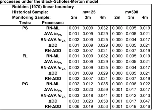
Table 1: Size of sequential change-point tests for different monitoring processes under the Black-Scholes-Merton model
Robbins (1970) linear boundary
Historical Sample: m=125 m=500 Monitoring Sample: 2m 3m 4m 2m 3m 4m Tests: Processes: PS RN-ML 0.001 0.009 0.032 0.000 0.005 0.019 ΔVA /σVA 0.001 0.009 0.029 0.000 0.005 0.021 RN-ΔVA /σVA 0.002 0.009 0.025 0.000 0.004 0.017 ΔDD 0.001 0.009 0.029 0.000 0.005 0.021 RN-ΔDD 0.002 0.007 0.021 0.000 0.007 0.019 FL RN-ML 0.001 0.009 0.032 0.000 0.005 0.019 ΔVA /σVA 0.001 0.009 0.029 0.000 0.005 0.021 RN-ΔVA /σVA 0.002 0.009 0.025 0.000 0.004 0.017 ΔDD 0.001 0.009 0.029 0.000 0.005 0.021 RN-ΔDD 0.002 0.007 0.021 0.000 0.007 0.019 PG RN-ML 0.002 0.012 0.035 0.000 0.006 0.022 ΔVA /σVA 0.003 0.023 0.059 0.001 0.017 0.047 RN-ΔVA /σVA 0.003 0.018 0.041 0.001 0.012 0.043 ΔDD 0.003 0.023 0.058 0.001 0.017 0.047 RN-ΔDD 0.006 0.019 0.053 0.001 0.019 0.046 Notes:
(1) The three sequential change-point tests are: Partial Sums (PS), Fluctuation (FL), Page (PG).(2) The monitoring processes are: Change in Distance to Default (ΔDD); Standardized changes in asset value (ΔVA /σVA) - while a constant volatility over the historical sample of m observations - the Radon-Nikodym derivatives based on the Maximum Likelihood mean estimator (RN-ML) on changes in Distance to Default (RN-ΔDD) and on Standardized changes in asset value (RN-ΔVA /σVA). (3) The number of replications is 1,000 with nominal size equal to 5%.(4) The ARHAC (den Haan and Levine,1997 ) with maximum lag length equal to 25 is estimated using the AIC. Similar results were obtained by the QSHAC with prewhitening (Andrews and Monahan, 1992). These HAC estimators used to scale statistics were estimated over the historical sample of m observations. Table 2: Power and Average Run Length (ARL) of sequential change-point tests for different monitoring
processes when there is a break in the mean value of the assets that follow a Black-Scholes-Merton model.
PS FL PG
Robbins (1970) linear boundary Monitoring Horizon = 4m
Break size in μVA : 2 3 4 2 3 4 2 3 4
Tests Process m Power ARL Power ARL Power ARL Power ARL Power ARL Power ARL Power ARL Power ARL Power ARL
RN-ML 125 138 0.838 51 0.911 24 0.933 15 0.838 51 0.911 24 0.933 15 0.844 48 0.914 23 0.935 15 ΔVA /σVA 0.835 51 0.908 24 0.930 16 0.835 51 0.908 24 0.930 16 0.842 48 0.911 23 0.932 15 RN-ΔVA /σVA 0.857 44* 0.934 15* 0.953 8* 0.857 44* 0.934 15* 0.953 8* 0.862 42* 0.936 14* 0.954 8* ΔDD 0.842 49 0.914 22 0.937 14 0.842 49 0.914 22 0.937 14 0.848 47 0.917 21 0.938 13 RN-ΔDD 0.748 84 0.901 27 0.936 14 0.748 84 0.901 27 0.936 14 0.724 93 0.891 31 0.941 12 RN-ML 500 550 0.903 98 0.937 47 0.948 31 0.903 98 0.937 47 0.948 31 0.907 92 0.939 44 0.949 29 ΔVA /σVA 0.903 98 0.937 47 0.947 31 0.903 98 0.937 47 0.947 31 0.907 92 0.939 44 0.949 29 RN-ΔVA /σVA 0.913 83* 0.949 29* 0.959 15* 0.913 83* 0.949 29* 0.959 15* 0.917 78* 0.950 28* 0.959 14* ΔDD 0.904 96 0.938 46 0.949 30 0.904 96 0.938 46 0.949 30 0.908 90 0.940 43 0.950 28
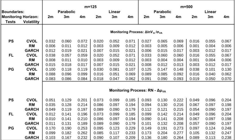
Table 3: Size of sequential change-point tests for monitoring the standardized changes in VA and the Radon-Nikodym (RN) derivative based on the estimated drift change
following the Heston model
m=125 m=500
Boundaries: Parabolic Linear Parabolic Linear
Monitoring Horizon: 2m 3m 4m 2m 3m 4m 2m 3m 4m 2m 3m 4m Tests Volatility Monitoring Process: ΔlnVA /σVA PS CVOL 0.032 0.060 0.072 0.020 0.052 0.071 0.027 0.065 0.069 0.016 0.055 0.067 RM 0.006 0.011 0.012 0.003 0.009 0.012 0.003 0.005 0.006 0.001 0.004 0.006 GARCH 0.012 0.019 0.021 0.007 0.015 0.021 0.006 0.015 0.017 0.003 0.012 0.017 FL CVOL 0.038 0.057 0.059 0.020 0.052 0.071 0.033 0.060 0.060 0.016 0.055 0.067 RM 0.008 0.011 0.010 0.003 0.009 0.012 0.003 0.004 0.004 0.001 0.004 0.006 GARCH 0.015 0.018 0.017 0.007 0.015 0.021 0.008 0.012 0.013 0.003 0.012 0.017 PG CVOL 0.100 0.118 0.119 0.030 0.081 0.107 0.125 0.147 0.148 0.038 0.101 0.130 RM 0.088 0.096 0.099 0.016 0.051 0.069 0.089 0.085 0.092 0.016 0.040 0.062 GARCH 0.083 0.086 0.084 0.018 0.047 0.062 0.091 0.090 0.093 0.019 0.050 0.070 Monitoring Process: RN - ΔμVA PS CVOL 0.051 0.129 0.201 0.073 0.099 0.185 0.093 0.130 0.222 0.049 0.096 0.204 RM 0.035 0.128 0.214 0.086 0.097 0.194 0.094 0.130 0.216 0.067 0.097 0.198 GARCH 0.049 0.119 0.197 0.089 0.090 0.179 0.112 0.121 0.215 0.054 0.090 0.197 FL CVOL 0.012 0.141 0.196 0.073 0.099 0.185 0.099 0.142 0.214 0.049 0.096 0.204 RM 0.010 0.141 0.210 0.086 0.097 0.194 0.090 0.141 0.208 0.067 0.097 0.198 GARCH 0.011 0.131 0.189 0.089 0.090 0.179 0.101 0.132 0.208 0.057 0.090 0.197 PG CVOL 0.170 0.190 0.253 0.095 0.123 0.229 0.149 0.191 0.273 0.097 0.124 0.248 RM 0.099 0.182 0.262 0.085 0.117 0.233 0.173 0.204 0.277 0.105 0.132 0.247 GARCH 0.103 0.167 0.232 0.090 0.107 0.209 0.136 0.180 0.264 0.089 0.113 0.238 Notes:
(1) The three sequential change-point tests are: Partial Sums (PS), Fluctuation (FL), Page (PG).
(2) The volatility models are: CVOL is the Constant Volatility, RM is the Riskmetrics with daily parameters a0=0.0, a1=0.94, a2=0.06 and the GARCH model with coefficients
a0=0.026, a1=0.844, a2=0.104.
(3) The number of replications is 1,000 with nominal size equal to 5%.
(4) The ARHAC (den Haan and Levine,1997 ) with maximum lag length equal to 25 is estimated using the AIC. Similar results were obtained by the QSHAC with prewhitening (Andrews and Monahan, 1992). The HAC estimators used to scale statistics were estimated over the historical sample of m observations. (5) The parabolic and the linear boundary correspond to the Chu et al (1996) and Zeileis et al (2005) boundaries, respectively.