RESEARCH ARTICLE
Robust optimal design of FOPID controller for
five bar linkage robot in a Cyber-Physical
System: A new simulation-optimization
approach
Amir ParnianifardID1☯*, Ali Zemouche2‡, Ratchatin ChancharoenID3‡, Muhammad Ali ImranID4‡, Lunchakorn Wuttisittikulkij1☯
*
1 Wireless Communication Ecosystem Research Unit, Department of Electrical Engineering, Faculty of Engineering, Chulalongkorn University, Bangkok, Thailand, 2 Wireless Communication Ecosystem Research Unit, Department of Mechanical Engineering, Faculty of Engineering, Chulalongkorn University, Bangkok, Thailand, 3 University of Lorraine, CRAN UMR CNRS 7039, Cosnes et Romain, France, 4 School of Engineering, University of Glasgow, Glasgow, United Kingdom
☯These authors contributed equally to this work. ‡ These authors also contributed equally to this work.
*[email protected](LW);[email protected](AP)
Abstract
This paper aims to further increase the reliability of optimal results by setting the simulation conditions to be as close as possible to the real or actual operation to create a Cyber-Physi-cal System (CPS) view for the installation of the Fractional-Order PID (FOPID) controller. For this purpose, we consider two different sources of variability in such a CPS control model. The first source refers to the changeability of a target of the control model (multiple setpoints) because of environmental noise factors and the second source refers to an anom-aly in sensors that is raised in a feedback loop. We develop a new approach to optimize two objective functions under uncertainty including signal energy control and response error control while obtaining the robustness among the source of variability with the lowest computational cost. A new hybrid surrogate-metaheuristic approach is developed using Particle Swarm Optimization (PSO) to update the Gaussian Process (GP) surrogate for a sequential improvement of the robust optimal result. The application of efficient global opti-mization is extended to estimate surrogate prediction error with less computational cost using a jackknife leave-one-out estimator. This paper examines the challenges of such a robust multi-objective optimization for FOPID control of a five-bar linkage robot manipulator. The results show the applicability and effectiveness of our proposed method in obtaining robustness and reliability in a CPS control system by tackling required computational efforts.
1. Introduction
Nowadays, developing processes in the engineering world is strongly associated with computer simulations. These computer codes can collect appropriate information about the characteristics
a1111111111 a1111111111 a1111111111 a1111111111 a1111111111 OPEN ACCESS
Citation: Parnianifard A, Zemouche A,
Chancharoen R, Imran MA, Wuttisittikulkij L (2020) Robust optimal design of FOPID controller for five bar linkage robot in a Cyber-Physical System: A new simulation-optimization approach. PLoS ONE 15(11): e0242613.https://doi.org/10.1371/journal. pone.0242613
Editor: Seyedali Mirjalili, Torrens University
Australia, AUSTRALIA
Received: August 19, 2020 Accepted: November 5, 2020 Published: November 30, 2020
Peer Review History: PLOS recognizes the
benefits of transparency in the peer review process; therefore, we enable the publication of all of the content of peer review and author responses alongside final, published articles. The editorial history of this article is available here:
https://doi.org/10.1371/journal.pone.0242613
Copyright:©2020 Parnianifard et al. This is an open access article distributed under the terms of theCreative Commons Attribution License, which permits unrestricted use, distribution, and reproduction in any medium, provided the original author and source are credited.
Data Availability Statement: The supplementary
materials including all Matlab®codes and functions and Excel data set and analysis required to
of engineering problems before actually running the process. Computer simulations can provide a rapid investigation of various alternative designs to decrease the required time to improve the system. In addition, most numerical analyses for engineering problems make a well-suited use of mathematical programming. The main goals of simulation include what-if study of a model or sensitivity analysis and optimization and validation of the model [1]. The essential benefit of simulation is its ability to cover complex processes, either deterministic or random while elimi-nating mathematical sophistication [2]. Clearly, because of the complexity of mathematical formulation analyzing in many real-world optimization problems, simulation-optimization methods become necessary to find more interest and popularity than other optimization meth-ods [3–5].
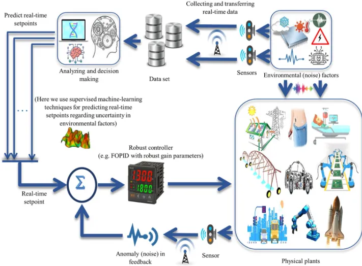
Cyber-Physical System (CPS) combines physical objects or systems with integrated compu-tational facilities and data storage [6]. CPS is a key enabling technology in systems intelligence. In CPS embedded computers and networks, the physical processes are controlled usually with feedback loops where physical processes affect computations and vice versa [7–10]. CPS is a multidimensional and complex system that integrates the cyber world with the dynamic physi-cal world. Integrating physiphysi-cal processes with computer systems is the main challenge pre-sented in CPS as the computational cyber part continuously senses the state of the physical system and applies decisions and actions for its control [11]. The integration and collaboration of three terms including computing, communication, and control are known as “3C” [12,13], CPS provides sensing, real-time optimization, information feedback, dynamic control, and other services, seeFig 1. In recent years, the application of CPS has been widely considered in different fields such as aerospace [14–16], defense [17,18], energy systems [19,20], healthcare [21–24], vehicle [25–27], and others [28–30].
In industrial practice, many CPS systems have been designed by decoupling the control sys-tem design. In this way, CPS and real-time interaction are achieved in order to monitor and control physical entities in a reliable, safe, collaborative, robust, and efficient way [12,13]. Using precise calculations to control a seemingly unpredictable physical environment is a great challenge [31]. After the CPS control system is designed and modeled by extensive simu-lation, tuning methods need to be expanded to address uncertainty and random disturbances in the system. In addition, ignoring the impact of uncertainty on the optimization model, the obtained optimal results may be far from the true optimum settings [32]. One of the main fea-tures in a reliable CPS design is the stability feature (robustness), which means no matter how the environment generates noise and uncertain factors, the control system should always reach a stable decision result eventually [33]. Robustness in the CPS control system seeks to achieve a certain level of performance with possible modeling errors in the forms of parametric or nonparametric uncertainties [34]. However, considering uncertainty and random distur-bances, while keeping the function and operation of the system, has been computationally time-consuming and costly.
Because of uncertainty, more complexity in the real-time control implementation of CPS is unavoidable. So, looking for less expensive computational methods of optimization consider-ing uncertainties has become interestconsider-ing among most engineerconsider-ing applications [35]. To over-come such computational difficulties, researchers have applied surrogate-based learning methods (e.g. polynomial regression, GP, and radial basis function) [36–39]. Surrogate-based methods can ‘learn’ the problem behaviors and approximate the function value. These approx-imation models can accelerate the function evaluation as well as the estapprox-imation of the function value with acceptable accuracy. Also, they can improve the optimization performance and pro-vide a better final solution. Various types of real-world engineering optimization problems have been developed by applying surrogate-based methods. These optimization problems include dynamic and stochastic control system design, sub-communities in machine learning
reproducing and replicating of our study’s findings have been shared publicly in the Zenodo repository via DOI and URL as below: DOI:10.5281/zenodo. 4266126URL:https://doi.org/10.5281/zenodo. 4266126.
Funding: This research project is supported by
Second Century Fund (C2F), Chulalongkorn University, Bangkok. The authors acknowledge the support by Second Century Fund (C2F), Chulalongkorn University, Bangkok for funding and postdoctoral fellowship to Amir Parnianifard (first and corresponding author). The funders had no role in study design, data collection and analysis, decision to publish, or preparation of the manuscript.
Competing interests: The authors have declared
problems, discrete event systems (e.g. queues, operations, and networks), manufacturing, medicine and biology, engineering, computer science, electronics, transportation, and logis-tics, see [3,5,38,40–42]. However, several studies have systematically illustrated the applica-tions of surrogate-based optimization algorithms [38,39,43–45].
In this paper, a new outline of robust real-time optimization in the CPS control model under the effect of environmental factors (also known as noise factors or uncertainty, see [4,
5]), and variability in feedback loop due to sensor’s anomaly is studied. The main contribu-tions of this study are as follows:
1. In this paper, we propose a new CPS framework of the control system for a five-bar linkage robot manipulator by considering the effect of uncertainty (sources of variability) in the sto-chastic model. The first source is related to a real-time setpoint that is predicted by learning from collected data (e.g. surrogate) over CPS environmental factors and the second vari-ability is found in output’s feedback due to anomaly in sensors. Besides, energy consump-tion and response error are optimized as a robust multi-objective optimizaconsump-tion model by Pareto frontier estimation in the real-time computational part of the CPS model.
Fig 1. Overall representation of Cyber-Physical System (CPS).
2. A new hybrid surrogate/metaheuristic algorithm for robust tuning of FOPID controller in the stochastic control system is proposed. The proposed hybrid GP/PSO algorithm has the advantages of both GP surrogates in learning the behavior of the model in an efficient global optimization with PSO metaheuristic in convergence searching for optimum results. We apply the straightforward jackknife leave-one-out technique to estimate surrogate pre-diction error applied in efficient global optimization.
3. The proposed algorithm can analyze the sensitivity of the obtained optimal results in such stochastic environments using the same collected data obtained among optimization procedure and simulation doesn’t need to be run anymore for computing the confidence intervals of robust optimal results (i.e. this algorithm does not to increase the number of function evaluations for sensitivity analysis).
The rest of this paper is organized as follows. Section 2 provides more details about real-time FOPID control when two types of uncertainties (noises) including environmental factors and sensor anomaly are considered in a CPS framework. Materials and methods of the pro-posed algorithm to handle robust multi-objective optimization of a CPS control system are elaborated in Section 3. In Section 4, the applicability and effectiveness of the proposed approach are examined to provide robustness and reliability in the robust optimal design of the FOPID controller in the CPS framework of a five-bar linkage robot manipulator. Finally, this paper is concluded in Section 6.
2. Point of view
The existing uncertainties and anomalies in the cyber environment have resulted in emerging concerns about the traditional control system [34]. In real-time control of CPS, physical pro-cess variables are monitored and propro-cessed by intelligent controllers for keeping the values of safety parameters between the given thresholds. Environmental conditions can affect system dynamics and also the controller function [9]. The precision of computing must interface with the uncertainty and the noise in the physical environment [46]. The physical world, however, is not entirely predictable. Normally, the CPS does not operate in a controlled environment. So, it must be robust to uncertainty (unexpected conditions) and adaptable to subsystem fail-ures [8].
2.1 Nomenclature
The main parameters and symbols used in the proposed algorithm are revealed inTable 1.
2.2 FOPID controller
In this paper, for better control, a fractional-orderPIλDμcontroller is used. Currently, frac-tional-order controllers are being extensively used by many scientists to achieve the most robust performance of the systems [47]. The main reason for choosing FOPID controllers is their additional degrees of freedom that result in a better control performance [48,49]. A generalized FOPID controller was first introduced by [50] which proposedPIλDμcontroller involving aλorder integer and aμorder differentiator. The differential equation of a frac-tional-orderPIλDμcontroller is defined by:
uðtÞ ¼KpeðtÞ þKiD l
t eðtÞ þKdD m
wheree(t) calculates an error value as the difference between a desired setpoint and a mea-sured process output in the time momentt. The controller attempts to minimize the error over time by adjustment of a control variableu(t). The reliability of the FOPID controller depends on the optimal design of three gain parameters (Ki,Kp,Kd) and two order parameters (λ,μ). However, we try to further increase the reliability of the tuning result by setting the traits of the simulation model to be as close as possible to the practical condition to make a CPS outline for the FOPID controller. The FOPID control system with a single setpoint does not express the aspects of the behavior that are essential to the system in the context of CPS. Moreover, we challenge the robust control to achieve CPS stability when the uncertainty in environmental conditions is the source of variability of the setpoints in the control system. In addition, an uncertain anomaly in sensors causes the noise (variability) in the control feedback loop. Moreover, we aim to tune the FOPID controller robustly in such a CPS control system with real-time setpoints and noise in the model’s feedback.Fig 2shows the control outline of CPS with real-time setpoints and noise in the model’s feedback. The application of the integer-order and fractional-integer-order of the PID controller in CPSs has been studied in [49,51–53].
Table 1. The table of nomenclature.
Notation Description
Ki,Kp,Kd, λ,μ
FOPID gain parameters (decision variables in an optimization model in this study).
e(t) The error of the control system in the time momentt(distance between the output of the system with the desired set point in time momentt).
bsðtÞ Desired setpoint in the control system (first uncertain variable in this study). ~
a Percent of variability in the feedback loop of the control system (second uncertain variable in this study).
Ls,Us The lower and upper limit for the uncertain variablebsðtÞ. Lα,Uα The lower and upper limit for the uncertain variable~a.
y(t) The output of the plant in a control system in the time momentt.
SEC Signal Energy Control
REC Response Error Control
F1,F2,OF First, second, and overall objective functions in the optimization model respectively.
θ A user-defined weighting factor used in overall function formulation and shows the tendency of the model towardF1orF2functions.
Means,Stds Mean and standard deviation ofsth input combination. Regarding the crossed array design, these statistical parameters are computed through repetitions ofsth input combination over different uncertainty scenarios.
SNRs Signal to noise ratio ofsth input combination and computed by SNRs¼10log½Means2þo�Stds2�.
ω A weighting parameter that is introduced to allow for individual emphasis on the minimization of variations inSNRsformulation.
l × m The number of simulation experiments regarding the structure of crossed array design withlinput combinations andmuncertainty scenarios.
EI(c) The expected improvement that can be considered for the candidate pointcfrom the best point so far.
γ Type I error and shows the probability of becoming infeasible from estimated confidence intervals.
Rp,s Performance measure criteria
CIs Confidence intervals for optimal result using the augmented bootstrapping technique (employ the same set of data used for optimization procedure).
b
Sc GP surrogate prediction error used in expected improvementEI(c) formulation. In this paper, the surrogate prediction error computed by the Jackknife leave-one-out approach.
2.3 Uncertainty in the CPS control model
Assume~z1ðtÞ;~z2ðtÞ;. . .;~znðtÞare the environmental (uncertain) factors in such a CPS control
outline. It should be noted that a real-time setpoint of the control system at time momenttis affected by variability on the environmental (uncertain) factors. Furthermore, the decision pol-icy needs to be able to predict real-time setpoints regarding the data collected from the uncer-tain environmental factors so far. Here, we use supervised learning of data collected so far from the environment (e.g. polynomial regression function,bf½~z1ðtÞ;~z2ðtÞ;. . .;~znðtÞ�Þand
predict the real-time setpointbs tð Þ ¼ddtbf;bs tð Þ 2½Ls;Us�in the control system. In addition, an
anomaly in the sensor to convey response feedback is assumed as uncertainty that causes the variability in the tuning of the FOPID controller. Assume that the true response of modely(t) is varied by~a%where~ais uncertain variableð~a2 ½La;UaÞ�, thus~yðtÞ ¼yðtÞ � ð1þ~aÞis a
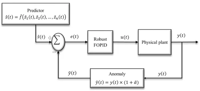
true response that is transmitted to the controller at time-stept.Fig 3shows a block diagram representation of the CPS control system by considering both types of uncertainty including environmental factors, and sensor anomaly.
Fig 2. The control framework of CPS with real-time setpoints and noise in model’s feedback. The environmental factors would be predicted and
applied as a real-time setpoint and anomaly in sensor is estimated in feedback loop. Gain parameters and order parameters in FOPID controller are tuned to be robust against source of variability.
2.4 Objective functions
This study aims at optimizing a robust multi-objective model of the FOPID tuning in the CPS framework by considering two different objective functions (e.g. performance criteria). The authors in [54] considered the amount of energy consumed to control the plant. They applied this measure to compare the optimal results obtained by different methods. However, they don’t use the energy consumption factor for the tuning procedure. Here, we define the Signal Energy Control (SEC) as the first objective function to optimize the energy that is consumed in the time domain 0�t�T:
F1 ¼ logðSECþ1Þ M1 ð2Þ and SEC¼ Z T 0 juðtÞjdt¼ Z T 0 jKpeðtÞ þKiD l t eðtÞ þKdD m teðtÞjdt ð3Þ
whereM1is a big value that is defined by user and is used to normalize the first objective
func-tion in [0,1], so thatM1>log(max0�t�TSEC).
We define the second objective function, namely Response Error Control (REC) inspired by common integral absolute error criteria [47,48] as below:
F2 ¼ logðRECþ1Þ M2 ð4Þ and REC¼ Z T 0 jeðtÞjdt¼ Z T 0 j~yðtÞ bsðtÞjdt ð5Þ
Fig 3. The block diagram of robust FOPID control in CPS framework with real-time setpoints and noise in model’s feedback. Real-time
setpoint is estimated by approximation function of environmental factors (~z1ðtÞ;~z2ðtÞ;. . .;~znðtÞ). Anomaly in sensor’s feedback is function of uncertain variableα~. FOPID gain parameters and order parameters are tuned robustly in such a way to make CPS insensitive against sources of variability in system.
whereM2shows a big value that is defined by user and is used to normalize the second
objec-tive function in [0,1], so thatM2>log(max0�t�TREC). Notably, we use a logarithmic scale for both objective functions to smooth the large differences between the values (i.e. cases in which one or a few points are much larger than the bulk of the data). As mentioned earlier, the real-time setpointbsðtÞinEq (5)can be predicted on-time by easy-to-apply supervised learning like polynomial regression as a function of environmental uncertain factor(s).
2.5 Overall objective function
To combine both objective functions including the signal energy control (seeEq (2)) with response error control (seeEq (4)) to be used as a single objective model, we applyLp-mertic approach byp= 2 (i.e. for more information aboutLp-mertic approach in multi-objective opti-mization, refer to [55]). Assumes= (1,2,. . .,l) is the vector of input combination, then we define the Overall Function (OF) as below:
OF¼ fyðF1Þ 2 þ ð1 yÞðF2Þ 2 g 1 2 ;for sð ¼1;2;. . .;lÞ ð6Þ whereθis a user-defined weighting factor (0�θ�1) that indicates the tendency of the model toward optimization based on each objective functionF1andF2, see Eqs (2) and (4).
Fluctuat-ing this magnitude (θ) provides the capture of Pareto frontier (also called Pareto optimal effi-ciency) to make a trade-off between each objective function. This approach is a classical method to solve optimization problems when the model is faced with multiple criteria [56]. In fact, the set of optimal solutions obtained from fluctuatingθin [0,1] provides an estimate of the Pareto frontier.
3. Proposed algorithm
In this section, we propose a promising technique for optimization under uncertainty using augmented efficient global optimization using the jackknife leave-one-out technique to esti-mate GP prediction error hybrid GP/PSO method. For this purpose, we first explain the main materials and methods used in the proposed algorithm briefly and then sketch the algorithmic steps in the proposed approach.
3.1 Materials and methods
3.1.1 Gaussian Process (GP) surrogate. GP which is also known as kriging is a
non-parametric Bayesian approach to supervised learning [57]. GP is an interpolation method that can cover deterministic data and is highly flexible due to its ability to employ various ranges of correlation functions [58]. In a GP model, a combination of a polynomial model and the reali-zation of a stationary point are assumed by the form of:
y¼fðXÞ þZðXÞ þε ð7Þ fðXÞ ¼X k p¼0 b bpfpðXÞ ð8Þ
where the polynomial terms offp(X) are typically the first or the second-order response surface approach and coefficientsbbpare regression parameters (p= 0,1,. . .,k). This type of GP approximation is called the universal GP, while in the ordinary GP, instead off(X), the constant meanμ=E(y(x)) is used. The termεdescribes the approximation error and the termZ(X) represents the realization of a stochastic process which in general is a normally
distributed Gaussian random process with zero mean, varianceσ2, and non-zero covariance. The correlation function ofZ(X) is defined by:
Cov½ZðxkÞ;ZðxjÞ� ¼s
2
Rðxk;xjÞ ð9Þ
whereσ2is the process variance andR(xk,xj) is the correlation function that can be chosen from different correlation functions which were proposed in the literature (e.g. exponential, Gaussian, linear, spherical, cubic, and spline), see [59,60]. Today, GP surrogate has been used as a widespread global approximation technique that is applied widely in control engineering design problems [40,61].
3.1.2 Particle Swarm Optimizer (PSO). The canonical PSO algorithm was proposed by
[62] and is inspired by the social behavior of swarms such as bird flocking or fish schooling. The parameters of PSO consist of the number of particles, position of agent in the solution space, velocity, and neighborhood of particles (communication of topology). The PSO algo-rithm begins with initializing the population. The second step is to calculate the fitness values of each particle, followed by updating individual and global bests as the third step. Then, veloc-ity and the position of the particles become updated (step four). The second to fourth steps are repeated until the termination condition is satisfied [63,64]. The PSO algorithm is formulated as follows [62–64]: vtþ1 id ¼w:v t idþc1:randð0;1Þ:ðptid x t idÞ þc2:randð0;1Þ:ðptgd x t idÞ and xtþ1 id ¼xtidþvt þ1 id ð10Þ wherewis the inertia weight factor,vt
idandx t
idare particle velocity and particle position
respec-tively.dis the dimension in the search space,iis the particle index, andtis the iteration num-ber. Expressionsc1andc2represent the speeds of regulating the length when flying towards
the most optimal particles of the whole swarm and the most optimal individual particle. The termpiis the best position achieved by particleiso far andpgis the best position found by the neighbors of particlei. The expressionrand(0,1) shows the random values between 0 and 1. The exploration happens if either or both of the differences between the particle’s bestðpt
idÞ
and previous particle’s positionðxt
idÞ, and between the population’s all-time bestðptgdÞand
pre-vious particle’s positionðxt
idÞare large. In addition, exploitation occurs when these two values
are both small. PSO has attracted wide attention in control engineering design problems due to its algorithmic simplicity and powerful search performance [54,65]. However, PSO algo-rithm that requires a large number of fitness evaluations before locating the global optimum is often prevented from being applied to computationally expensive real-world problems [66]. Therefore, surrogate-assisted PSO metaheuristic optimization algorithms have been focused in the literature, see [66–68].
3.1.3 Uncertainty management. Here, we follow [39,69,70] and inspire Taguchi’s
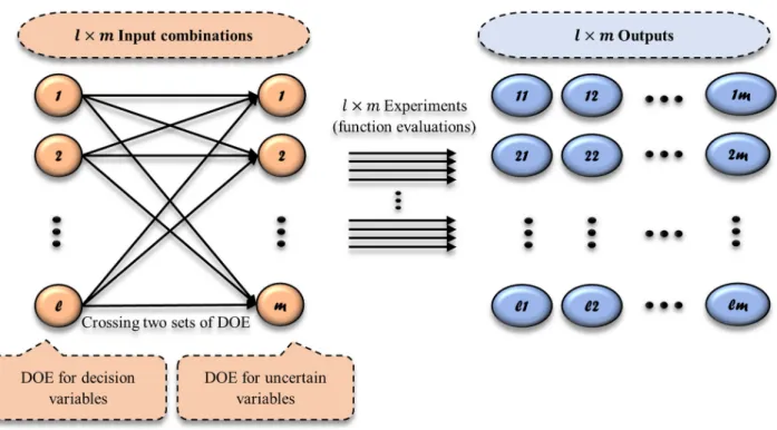
over-view of robust design [71] for dealing with uncertainty as a source of variability in the model. However, we expand Taguchi’s robust design terminology and apply its definition for environ-mental noise factors in such a CPS control system. But in this study, we replace the statistical approach of Taguchi viewpoint with augmented efficient global optimization using jackknife leave-one-out technique and hybrid GP/POS approach. Furthermore, we first intersect two sampling design sets. One sampling design is for decision variables (inner array) and another is for uncertain variables (outer array). Given thats= (1, 2,. . .,l) is the vector of sample points
over decision variables, andr= (1, 2,. . .,m) is the vector of uncertainty scenarios, sol×m input combinations are designed, and the real model (or true simulation model) are evaluated l×mtimes to collect relevant simulation outputs, seeFig 4. AssumeYis thel×mmatrix of simulation outputs (i.e. in this study the simulation outputs include OF values that can be
obtained regardingEq (6)), thus mean and standard deviation (Std) for each arrow inYcan be computed by the following equations:
Means¼ 1 m Xm r¼1 ysr ;for ðs¼1;2;. . .;lÞ ð11Þ Stds¼ ffiffiffiffiffiffiffiffiffiffiffiffiffiffiffiffiffiffiffiffiffiffiffiffiffiffiffiffiffiffiffiffiffiffiffiffiffiffiffiffiffiffiffiffiffiffiffiffiffi 1 m Xm r¼1 y2 sr 1 m Xm r¼1 ysr !2 v u u t ;for ðs¼1;2;. . .;lÞ ð12Þ
Signal-to-Noise Ratio (SNR) as introduced by Taguchi [71,72] is a robustness criterion based on the mean and the Std of a system responseY. Given that,Yis the smaller the better type, Taguchi assumed zero as the minimal possible response value. Accordingly, he formu-lated the following SNR as the robustness criterion:
SNRs¼10log½Means2þo�Stds2� ;for ðs¼1;2;. . .;lÞ ð13Þ
Since we performed a minimization of the model’s output (here is the overall function, see
Eq (6)) to find the optimal parameters of the FOPID controller, the formulation of the SNR in
Eq (13)has the opposite sign by Taguchi formulation. Additionally, a weighting parameterω is introduced to allow for individual emphasis on the minimization of variations. The smallest value of SNR inEq (13)depicts the better point with smaller relevant simulation output and higher insensitivity to the source of variability (robustness).
3.1.4 Efficient global optimization using a jackknife leave-one-out strategy. A common
formulation of efficient global optimization has been developed in the outline of the expected
Fig 4. Crossing two sets of DOE dealing with uncertainty in a model, one DOE (lsamples) over decision variables of the model and second DOE (msamples) over uncertain variables in the model.
improvement criterion, see [73,74]. The expected improvement (EI) method has been devel-oped in engineering design problems to adaptively improve the local and global search of opti-mal points (i.e. control a trade-off between exploration and exploitation properties) [75]. This method has been combined with two main parts. The first statistical part consists of the design of experiments and surrogate techniques and the second part involves evolutionary algorithms. IfSNRcis considered for the arbitrary pointc, an improvement function over the best point
that is so far computed withSNRbis defined asmax{0, (SNRb−SNRc)}. A common
formula-tion of efficient global optimizaformula-tion in term of expected improvement creaformula-tion is constructed as below: EIðcÞ ¼ ðSNRb SNRdcÞF SNRb SNRdc b Sc ! þbSc; SNRb SNRdc b Sc ! ð14Þ
whereSbcindicates the estimation of GP perdition’s error on candidate pointc. The
expres-sionSNRbshows the value of the best signal to noise ratio that is obtained from true data of the original simulation model, andSNRdcis GP surrogate prediction on candidate pointc. The termsFand;depict the cumulative distribution function (CDF) and probability den-sity function (PDF) of a standard normal distribution respectively. The first phrase (F) in
Eq (14)is related to the local search and the second phrase (;) is related to a global search. In the search for the next best point among all the candidate points, the point with maxi-mum EI term inEq (14)is selected and replaced with the best point so far obtained. This procedure is continued untilMax REI−0�ε, whereεis a user-defined threshold, or an allocated computational cost (e.g. fixed number of repetitions) is reached. However, to find the neighbor points (candidate points) around the current best point, different strategies of sampling design methods can be used such as factorial designs [76] and space-filling design [77]. Here, we apply PSO global optimizer to investigate the maximum EI among the whole design space.
In order to estimate the surrogate prediction error forcth candidate pointðSbcÞinEq (14),
simulation experiments can be resampled [73,74]. The authors in [77] have used the boot-strapping technique to obtain perdition error for a GP surrogate using resampling to refit sur-rogate and obtain prediction error. However, resampling imposes extra computational cost due to the additional number of required simulation experiments (function evaluations). Here, to estimate the surrogate prediction error for each candidate point, we apply the jack-knife leave-one-out approach. This approach applied an available set of I/O data and doesn’t need resampling and extra simulation experiments.
3.1.5 Jackknife leave-one-out approach. Jackknife was first introduced by Quenouille
(1949) [78] and named by Tukey (1958) [79]. The application of the jackknife method involves a leave-one-out strategy for the estimation of a parameter (e.g. the variance) in a dataset [80]. In this study, we are motivated to use the jackknife leave-one-out approach to estimate surro-gate prediction errorðbScÞrequired inEq (14)formulation, because this method uses an exist-ing data and does not require to re-run the expensive simulation model. Here, this method is used to predict GP prediction error while it can be used for other surrogates as well. LetSNRdc denotes the prediction of GP surrogate that fitted over alllsamples (input combinations), therefore the GP perdition error incth candidate pointðbScÞcan be estimated through the jack-knife leave-one-out approach as the steps in Algorithm 1.
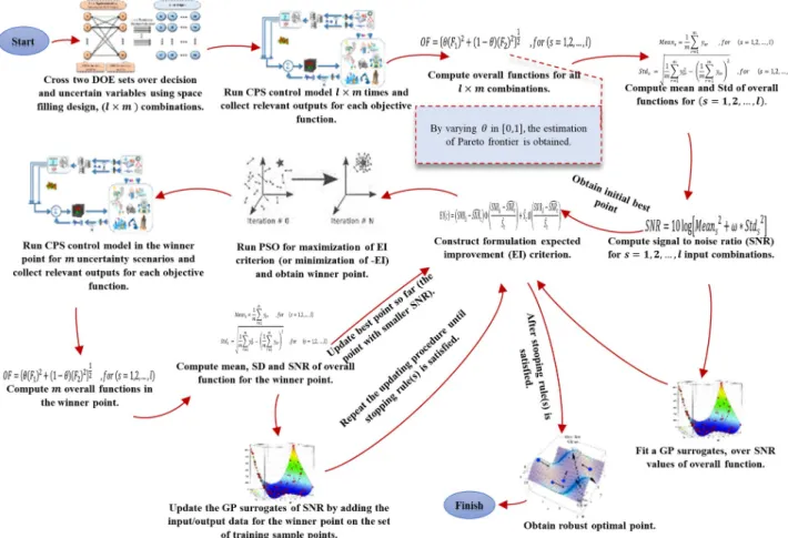
3.2 Algorithmic framework
In this study, we develop a new hybrid surrogate/metaheuristic method applied in robust effi-cient global optimization and optimization under uncertainty. We apply a PSO metaheuristic to update a GP surrogate for sequential investigation of a robust optimal point. The proposed algorithm can handle robust efficient global optimization by the exhaustive search method that can be applied in real operation of CPS control frameworks. The algorithmic representa-tion of the proposed approach is presented inFig 5. The main steps involved in the proposed algorithm are presented in Algorithm 2. Note that, we assume the approximation function fit-ted over environmental factorsbfð~z1ðtÞ;~z2ðtÞ;. . .;~znðtÞÞcan be used to estimate upper (Us) and lower bound (Ls) forbsðtÞby varying~z1ðtÞ;~z2ðtÞ;. . .;~znðtÞin their relevant ranges (upper
and lower bounds of each relevant environmental factor) in time-stept. Here, these bounds are predefined and existed as inputs of the program.
Algorithm 1. Jackknife leave-one-out approach.
Input: Set of input combinations and relevant output (SNR).
Output: Estimation of surrogate prediction error for cth candidate point.
begin
Step 1. Select lc samples from the complete set of l combinations
(s = 1, 2, . . .,l) when ic = l − k and k is a set of samples located in
vertices (i.e. we aim to avoid extrapolating of GP surrogate).
Fig 5. Algorithmic representation of proposed approach for hybrid GP-PSO based robust simulation-optimization under uncertainty.
Step2: Drop uth samples (simulation experiment) and relevant SNR output when (u = 1, 2, . . ., ic).
Step 3: Fit a new GP surrogate over (lc − 1 + k) remaining samples.
Step 4: Predict output for cth candidate point (SNRd u
c Þ using the GP surrogate constructed from the previous step.
Step 5: Implement three previous steps for all lc samples computing lc relevant predictions.
Step 6: Apply the jackknife estimator to obtain the estimation of surrogate prediction error for cth candidate point as below:
b Sc� 1 lc Xlc u¼1 ðSNRdc SNRd u c Þ 2 ( )1=2 End
Algorithm 2. Proposed robust simulation-optimization approach.
Input: Estimated upper (Us) and lower bound (Ls) for system’s setpoint
bsðtÞ 2 ½Ls;Us� and upper (Uα) and lower bound (Lα) for ~a due to anomaly in
sensor feedback.
Output: The estimation of the Pareto frontier by a set of robust opti-mal points found by the proposed approach.
begin
Step 1. Design crossed array (using the space-filling design) by crossing two sets of experiments with dimensions l × m as below: • An inner array matrix with dimension (l×nx) wherelis the number of sample points for
decision variables andnxis number of decision variables (e.g. in FOPID tuningnx= 5 deci-sion variables including three gainKi,Kp,Kdand two orderλ,μparameters).
• An outer array matrix with dimension (m×nz) where m is the number of sample points
(uncertainty scenarios) for nzuncertain variables (e.g. here in represented CPS control
sys-tem nz= 2 includingbsðtÞand~a).
Step 2. Run the CPS model (i.e. here we use simulation model) for each crossed (l × m) combination and obtain the relevant output bysr
regarding each objective function, when s = (1, 2, . . ., l) and r = (1, 2, . . ., m).
Step 3. Compute overall function (OF) values for all l × m input com-binations using Eq (6).
Step 4. Compute Means and Stds of overall function using Eqs (11) and
(12) for each s = (1, 2, . . ., l) sample point in inner array and compute relevant SNRs using Eq (13).
Step 5. Fit a GP surrogate over sets of I/O data (with l input combi-nations and relevant SNRs values).
Step 6. Define an initial best point among the set of I/O data obtained from Step 4 (the point with the smallest SNR regarding Eq (13)).
Step 7. Set expected improvement criterion (see Eq (14)) as an objec-tive function in PSO optimizer algorithm (i.e. with minimizing of −EI (c)) and obtaining a winner point.
Step 8. Run the real CPS model (e.g. original simulation model) in the winner point for m combinations of uncertainty (scenarios) designed in Step 1 and obtain relevant outputs for each objective function.
Step 9. Obtain OF values for the winner point regarding m uncertainty scenarios.
Step 10. Compute mean and Std of the winner point using Eqs (11) and (12).
Step 11. Update the set of I/O data s = (1, 2, . . ., l + i), when i is the number of the sequential runs.
Step 12. Fit a new GP surrogate over an updated set of I/O data (with l + i training points and SNR as outputs).
Step 13. Update (if needed) the best point obtained so far to a point with smallest SNR ratio among all the sample points (including initial training points and points which are added so far for updating of sur-rogate, see Step 11) and repeat Step 7 till Step 12 until stopping rules are satisfied (e.g. stop sequential updating if Max EI − 0 � ε, or i � k, where ε and k are user-defined thresholds).
Step 14. If stopping rule(s) is satisfied, then set the best point obtained so far as a robust optimal point of the model. The best point so far has the smallest SNR value among all sample points including initial samples and updating sample points.
Step 15. Obtain estimation of Pareto frontier by varying the weight scale θ in [0,1] (see Eq (6)) and repeating Step 1 to Step 14.
end
In this study, we use a common space-filling design method named Latin hypercube sam-pling (LHS) with the desired correlational function to design simulation experiments. LHS was first introduced by McKay and colleagues [81]. It is a strategy to generate random sample points while guaranteeing that all the portions of the design space are depicted. LHS has been commonly defined for designing computer experiments based on the space-filling concept. In general, forninput variables,msample points are produced randomly inmintervals or sce-narios (with equal probability). Inspired by [82] in the case of non-independent multivariate input variables, the desired correlation matrix can be used to produce distribution-free sample points in LHS. For more information, refer to [39,83].
In the represented CPS control system in this study, outputs for two separateF1andF1
objective functions need to be obtained regarding response error control and signal energy control, see Eqs (2) and (4). Notably, in Step 4, eachs= (1,2,. . .,l) sample point is repeatedm times throughmdifferent combinations (scenarios) of uncertain variables, see the framework of uncertainty management in Section 3.1.3. In Step 7, the fitted GP surrogate over SNR con-structed in Step 5 is used to approximate the relevant SNR of each search point produced by PSO.
3.3 Augmented bootstrapping approach (sensitivity analysis)
In this study, the main idea behind the proposed algorithm is to perform sensitivity analysis to expand the information obtained from robust efficient global optimization. Estimating a single optimal point using a particular response may be inaccurate because of variability in the surrogate. Thus, we derive a series of possible responses that take into account a degree of uncertainty by providing confidence regions or prediction intervals. The author in [84] has mentioned two alternative strategies for bootstrapped resampling as follows:
• In each set of bootstrapping, both sets of input (design) combination (X) and noise (uncer-tain) combination (Z) are resampled randomly.
• The resampling is adapted to noise or uncertain component (Z) only while keeping the deterministic input combination (X) fixed.
Here, to find the bootstrapped set of data, a model is resampledBtimes (b= 1,2,. . .,B) (sampling with replacement), whileBis the number of resampled or bootstrapped sample size. Moreover,Bseparate surrogates are fitted onBdifferent sets of sample points with the same size (ndesign points). It is assumed thatd+is a robust optimal solution which is obtained from the original (non-bootstrapped) surrogate. All output values in pointd+are estimated using all theBbootstrapped surrogates. The distribution-free bootstrapped Confidence Intervals (CIs)
can be computed as below, [59,85]: Pðdþ� ðbBðgÞcÞ�d þ �dþ� ðdBð1 ðg=2ÞeÞÞ ¼1 g ð15Þ
The superscript ‘�’ is a common symbol for bootstrapped values [59]. The expressionγ gives two-sided CIs. Bonferroni’s inequality suggests that Type I error rate for each interval per output is divided by the number of outputs (here is SNR). If the values of bootstrap esti-mateSNR(d+)�are sorted from low to high, thenb.candd.erespectively denote floor and ceil-ing function to achieve the integer part and round upwards.
Here, inspired by [70,86], the particular augmented bootstrapping approach is used for costly simulation running. In such a case, assume the set of sample points is fixed and only old data to fit surrogate with enough replication is available and new simulation replicating is very expensive. This augmented bootstrapping approach does not imply extra computational cost because of resampling and required simulation running to find a bootstrapped set of data.xs (s= 1,2,. . .,l) denotes the set of sample points and eachxsis repeatedmtimes (r= 1,2,. . .,m). We assume that the original set of data obtained from the original simulation model is avail-able (sizel×m) whenmis the number of scenarios for uncertainty andlis the number of input combinations. Moreover, the augmented bootstrapping procedure is sketched in Algo-rithm 3.
Algorithm 3. The augmented bootstrapping procedure. Input: Set of I/O data, and robust optimal point. Output: Estimation of CIs.
begin
Step 1. Set s = 1 and r = 1.
Step 2. Choose (with replacement) one random number from the collec-tion of {r� = 1, 2, . . ., m}.
Step 3. Replace the rth original output ys,r (selected from the old data) with the bootstrap outputy�
s;r¼ys;r�.
Step 4. Set r = r + 1 and continue Step 3 and Step 4 till r = m. Step 5. Set s = s + 1 and continue Step 3, Step 4 and Step 5 till s = l.
Step 6: Compute Mean� s;Std
�
s, and SNR �
using Eqs (11), (12) and (13) respectively for (s = 1, 2, . . .l) and fit a GP surrogate over new set of I/O data.
Step 7: Continue resampling B times (b = 1, 2, . . ., B) where B is the number of resampling or bootstrap sample size and compute
SNR� b¼ ðSNR � 1;SNR � 2;. . .;SNR � bÞ.
Step 8: Compute bootstrapped CIs using Eq (15) for the robust optimal point obtained by the proposed algorithm as elucidated in Section 3.2).
end
Note that, regarding the Step 1 till Step 5, it can be seen that a random number with replace-ment in [1,m] is selected, and regarding the selected number, we choose the relevant response in an outer array (see the structure of the crossed array design explained in Section 3.1.3) that was previously collected from the original simulation model and has the same column num-ber. For the same input combination, we repeat this proceduremtimes and collectmdifferent responses or may have the same responses (i.e. because the random selection is done with replacement). This procedure is also repeated for other input combinations. Therefore, the data matrix withlrow andmcolumn is constructed.
4. Numerical example
Here, the proposed algorithm is specified for the robust optimal design of FOPID controller in CPS control of five-bar linkage robot manipulators. In the continue, we first explain the dynamics of the five-bar linkage robot manipulators. Next, the robust optimal design of FOPID controller in the CPS framework of a five-bar linkage robot manipulator is obtained using the proposed algorithm in this paper.
4.1 Dynamics of a five-bar linkage robot manipulator
Robotic manipulators, classic examples of nonlinear systems, are extensively used in the indus-try to automate various aspects of the production process of goods, thereby improving the quality of human life [87]. With the changing dynamics of these manipulators and their increasing complexity arising from their greater use, there has been considerable interest in their control technique fields. Robotic manipulators are Multi-Input Multi-Output (MIMO) systems with highly coupled nonlinear dynamics, posing a challenge to the development of their control scheme [88]. A five-bar linkage manipulator is a special class of parallel manipu-lators where a minimum of two kinematic chains control the motion of end-effectors [89]. The mechanism of a five-bar linkage is shown inFig 6[90].
Even though there are four links being moved, there are in fact only two degrees-of-free-dom that are defined asq1andq2.qiandτiare the joint variable and torque of theith motor
Fig 6. Five bar linkage robot manipulator.
respectively. Likewise,Ii,li,lci, andmiare the inertia matrix, length, distance to the center of gravity, and mass of theith link respectively. In addition, ifm3l2lc3=m4l1lc4, then the inertia
matrix is diagonal and constant. As a consequence, the dynamic model of the manipulator is derived by the following equations [90]:
t1¼ d11q€1þgcosq1ðm1lc1þm3lc3þm4l1Þ
t2¼ d22q€2þgcosq2ðm1lc1þm3lc3þm4l1Þ
ð16Þ where g is gravitational constant andd11andd22are as follows:
d11¼ m1l 2 c1þm3l 2 c3þm4l 2 1þI1þI3 d22¼ m2l 2 c2þm4l 2 c4þm3l 2 2þI2þI4 ð17Þ
It should be noted thatτ1depends only onq1but not onq2. Similarly,τ2depends only on
q2but not onq1. This discussion helps to explain the popularity of the parallelogram
configu-ration in industrial robots. Ifm3l2lc3=m4l1lc4, then two anglesq1andq2can be adjusted
inde-pendently without worrying about interactions between the two angles.
4.2 Simulation and algorithm setup
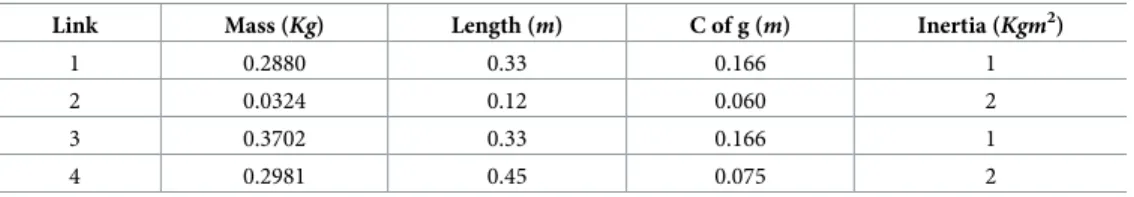
Here, the main goal is to obtain a robust optimal design of FOPID controller in such a CPS control model as elucidated in Section 2. We simulate the five-bar linkage robot manipulator usingEq (16)in Matlab1/Simulink environment. Simulink does not have a library for the FOPID. Therefore, the controller from the library of FOMCON: a Matlab1toolbox for frac-tional-order system identification and control [91], which allows for the computation of the fractional-order derivative and integration is used. Numeric values of the parameters of the five-bar manipulator dynamics are taken from [54,92] as shown inTable 2. From the data that are driven inTable 2, it is revealed thatm3l2lc3=m4l1lc4, thus we can perform robust optimal
design of controller for one motor, where the same results are also valid for the second motor. In FOPID tuning, five decision variables includingKi,Kp,Kd,λ, andμare considered as deci-sion variables. The search procedure for the robust optimal result is done in the ranges as [54]:
Kp2 ½0;30�;Ki2 ½0;5�;Kd2 ½0;5�;m2 ½0;1�and l2 ½0;1�
Two performance criteria are considered as outputs of the model including Eqs (2) and (4) in time-stept(here the size of time-step is fixed at 0.01) and time domain (simulation time) T= 20. In addition, for uncertain variables, we assume thatbsðtÞvaries in [0.5,2.5] anda~varies in [−0.05,0.05]. However, we implement the proposed algorithm in CPS control framework of a five-bar linkage robot manipulator.
The following process is done to determine the robust optimal values of the FOPID param-eters (Ki,Kp,Kd,λ, andμ) using the proposed algorithm. First, we design a set of experiments with the size ofl= 15 samples using LHS. Another sampling design is constructed for
Table 2. Numeric values of the parameters of the five-bar manipulator dynamics.
Link Mass (Kg) Length (m) C of g (m) Inertia (Kgm2)
1 0.2880 0.33 0.166 1
2 0.0324 0.12 0.060 2
3 0.3702 0.33 0.166 1
4 0.2981 0.45 0.075 2
uncertain factorsbsðtÞand~a(here we choosem= 9 samples as the size of uncertainty scenar-ios). Two Matlab1functions “lhsdesign” and “gridsamp” are used to design training sample points with minimum correlation and to design uncertainty scenarios (different combinations of uncertain factors) respectively. We cross both sets of experiments to follow the crossed array design framework as elaborated in Section 3.1.3. Each input combination in the inner arrays= (1,2,. . .,l= 15) including designed values ofKi,Kp,Kd,λ, andμare sent to Simulink block formtimes regarding each uncertainty scenariosr= (1, 2,. . .,m= 9) and the values of SEC and REC in time domain are collected. So, 15×9 simulation outputs are collected accord-ing to 135 simulation runs (function evaluations). We, use the collected data to obtainF1,F2,
and, OF regarding Eqs (2), (4) and (6) respectively. We set bothM1andM2parameters equal
to 10 used in Eqs (2) and (4). Regardingmuncertainty scenarios, we repeat each input combi-nationmtimes, and compute the relevant mean and Std of OF using Eqs (11) and (12). Then, we calculateSNRsfor each input combinations= (1,2,. . .,l= 15) usingEq (13)while assume
ω= 3. Afterwards, we fit a GP surrogate over set of input combinations and set ofSNRs out-puts. The DACE [93], Matlab1toolbox has been employed to construct GP surrogate. In the current study, first-order polynomial regression and Gaussian correlation functions are adjusted to fit GP surrogate. The correlation parameter is fixed on 0.1 (i.e. in the DACE tool-box, the correlation parameter is forced to vary in the range between 0.01 to 20).
Next, we perform the procedure of sequential expected improvement to estimate the robust optimal point afternsequential EI iterations. Among all theSNRvalues in the set ofSNRs, a sample with the smallestSNRvalue and its relevant input combination including the relevant vector of [Ki,Kp,Kd,λ,μ] is considered as an initial best point. Regarding our proposed algo-rithm, we apply the PSO optimizer to search for a winner point in each sequential EI iteration. For setting the PSO parameters, the maximum iteration number is fixed 200 and the swarm is initialized with 30 particles. Notably, as we use GP surrogate instead of the true (original) sim-ulation model as an objective function in PSO, thus we don’t worry about the computational cost due to running of a true simulation model. At the end of any sequential EI iteration, the program checks the stopping rule(s). Here, we stop the EI procedure when the EI criterion becomes smaller than 0.01, or the number of sequential runs reaches 15 iterations. Also, at the end of any sequential EI iteration, two terms of the program are updated, i) the set of training sample points by adding a winner point and relevant SNR output that is computed accordingly from the original simulation model, ii) the best sample point obtained so far with the smallest SNR among all the training points and updating points. Moreover, according to an updated set of training samples, a new GP surrogate is constructed after each sequential EI iteration. It is important to note that we avoid extrapolation of GP surrogate in each sequential iteration by setting two different rules, i) we consider a death penalty for any point that is investigated by PSO and is located out of bounds of training points, ii) to estimate GP prediction error using jackknife leave-one-out approach, we only remove input combination’s rows that don’t locate on the margin of design space (see Section 3.1.5). The obtained results from the pro-posed algorithm and relevant sensitivity analysis are discussed in the following sections.
4.3 Robust optimal results
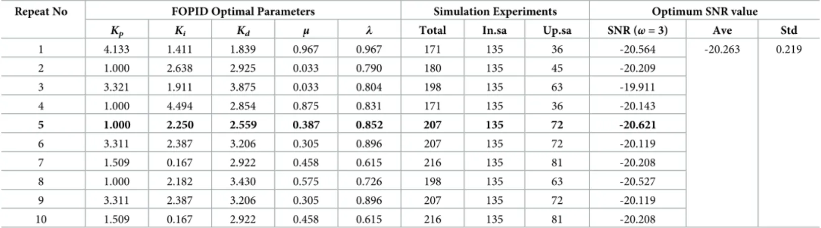
We perform the proposed algorithm for three different values ofθ= 0.25,θ= 0.5, andθ= 0.75 in computing OF (seeEq (6)). To evaluate the effect of randomness in sampling design meth-ods, each optimization set was repeated 10 times. Tables3–5show the obtained results using the proposed algorithm for estimating robust FOPID optimal design over 10 different repeti-tions forθ= 0.25,θ= 0.5, andθ= 0.75 respectively. As mentioned in Section 4.2, the obtained SNR values are computed by repeating each set of FOPID gain parameters over 9 different
uncertainty scenarios designed by the grid sampling method. In those tables, two expressions “In.sa” and “Up.sa” indicate the initial sampling design and updating samples that are added to the training set through the procedure of sequential improvement respectively.
As can be seen, forθ= 0.25, the best SNR (−20.621) is obtained through the fifth repetition with a total of 207 function evaluations (15×9 runs regarding initial crossed sampling design
Table 3. Robust FOPID optimal results using proposed algorithm for 10 repetitions forθ= 0.25 (the results obtained over 9 different uncertainty scenarios).
Repeat No FOPID Optimal Parameters Simulation Experiments Optimum SNR value
Kp Ki Kd μ λ Total In.sa Up.sa SNR (ω= 3) Ave Std
1 4.133 1.411 1.839 0.967 0.967 171 135 36 -20.564 -20.263 0.219 2 1.000 2.638 2.925 0.033 0.790 180 135 45 -20.209 3 3.321 1.911 3.875 0.033 0.804 198 135 63 -19.911 4 1.000 4.494 2.854 0.875 0.831 171 135 36 -20.143 5 1.000 2.250 2.559 0.387 0.852 207 135 72 -20.621 6 3.311 2.387 3.206 0.305 0.896 207 135 72 -20.119 7 1.509 0.167 2.922 0.458 0.615 216 135 81 -20.208 8 1.000 2.182 3.430 0.575 0.726 198 135 63 -20.527 9 3.311 2.387 3.206 0.305 0.896 207 135 72 -20.119 10 1.509 0.167 2.922 0.458 0.615 216 135 81 -20.208 https://doi.org/10.1371/journal.pone.0242613.t003
Table 5. Robust FOPID optimal results using proposed algorithm for 10 repetitions forθ= 0.75 (the results obtained over 9 different uncertainty scenarios).
Repeat No FOPID Optimal Parameters Simulation Experiments Optimum SNR value
Kp Ki Kd μ λ Total In.sa Up.sa SNR (ω= 3) Ave Std
1 8.238 2.300 3.748 0.426 0.919 261 135 126 -23.868 -24.041 0.140 2 1.267 3.101 3.332 0.525 0.835 270 135 135 -24.238 3 4.285 1.998 3.510 0.612 0.938 189 135 54 -24.032 4 7.803 3.239 3.257 0.944 0.918 216 135 81 -24.191 5 1.025 2.144 3.072 0.567 0.860 270 135 135 -24.151 6 6.113 1.314 3.039 0.709 0.967 243 135 108 -24.022 7 5.775 2.308 3.689 0.348 0.913 234 135 99 -23.879 8 5.201 2.485 4.124 0.823 0.794 261 135 126 -24.213 9 5.775 2.308 3.689 0.348 0.913 234 135 99 -23.879 10 11.00 1.833 2.833 0.900 0.967 270 135 135 -23.939 https://doi.org/10.1371/journal.pone.0242613.t005
Table 4. Robust FOPID optimal results using proposed algorithm for 10 repetitions forθ= 0.5 (the results obtained over 9 different uncertainty scenarios).
Repeat No FOPID Optimal Parameters Simulation Experiments Optimum SNR value
Kp Ki Kd μ λ Total In.sa Up.sa SNR (ω= 3) Ave Std
1 3.321 1.549 2.634 0.967 0.967 225 135 90 -21.838 -21.840 0.245 2 1.000 0.713 2.017 0.802 0.726 261 135 126 -22.249 3 1.000 2.668 3.604 0.575 0.832 225 135 90 -21.879 4 1.000 1.228 2.436 0.657 0.844 189 135 54 -22.120 5 1.000 2.667 3.947 0.696 0.757 225 135 90 -21.949 6 3.429 1.782 3.410 0.298 0.861 243 135 108 -21.562 7 7.000 1.833 2.833 0.433 0.967 198 135 63 -21.448 8 1.000 1.964 3.909 0.775 0.705 180 135 45 -22.003 9 3.740 1.702 2.151 0.033 0.915 189 135 54 -21.551 10 2.233 1.624 2.000 0.318 0.967 180 135 45 -21.803 https://doi.org/10.1371/journal.pone.0242613.t004
and 8×9 simulation runs regarding sequential updating of the training sample set). Forθ= 0.5, the best SNR (-22.249) is obtained from the second repetition and with a total of 261 simulation experiments (135 initial samples plus 126 updating samples). The best SNR value (-24.238) forθ= 0.75 is obtained through the second repetition by a total of 270 function eval-uations (15 initial input combinations and 15 update combinations that are crossed by 9 uncertainty scenarios). We consider all the three best points over all 10 repetitions as robust optimal points for the FOPID controller using the proposed algorithm for eachθ= 0.25,θ= 0.5, andθ= 0.75 separately.Fig 7shows the magnitudes of the EI criterion and the best SNR obtained by sequential expected improvement over 10 different repetitions of the proposed algorithm forθ= 0.25,θ= 0.5, andθ= 0.75. Also, the mean and Std of OF related to the best point so far (smaller SNR) in each sequential EI iteration are shown inFig 8. It should be noted that two stopping rules are adjusted, the EI value becomes smaller than 0.01, or the sequential procedure reaches 15 sequential iterations.Fig 9shows the step responses of the robot manipulator with 9 different uncertainty scenarios (bsðtÞ ¼ ½0:5;1:5;2:5�and
~
a¼ ½ 0:05;0;þ0:05�) forθ= 0.25,θ= 0.5, andθ= 0.75.
4.4 Sensitivity analysis
To analyze the sensitivity of robust optimal results obtained by the proposed algorithm and estimate the variability which occurred due to randomness in designing sample points, we used the augmented bootstrapping method explained in Section 3.3. Here, based on the obtained results from the original GP surrogate, the FOPID parameters in robust optimum point (d+) forθ= 0.25,θ= 0.5, andθ= 0.75 are defined as below:
Fig 7. EI criterion magnitudes and best SNR obtained by sequential expected improvement over 10 different repetition of proposed algorithm forθ= 0.25,θ= 0.5 andθ= 0.75. Two stopping rules are adjusted, EI value becomes smaller than 0.01 or reach 15 sequential
iterations.
• For,θ= 0.25 dþ¼ fK p¼1:00;Ki¼2:250;Kd¼2:259;m¼0:387and l¼0:852g SNRðdþ Þ ¼ 20:621 • Forθ= 0.5 dþ ¼ fKp¼1:00;Ki¼0:713;Kd¼2:017;m¼0:802and l¼0:726g SNRðdþÞ ¼ 22:249 • Forθ= 0.75 dþ ¼ fKp¼1:267;Ki ¼3:101;Kd¼3:332;m¼0:525 and l¼0:835g SNRðdþ Þ ¼ 24:238
WithBpredicted values fromBbootstrapped GP surrogates, we can quantify the CIs (boot-strapped confidence intervals) ford+. For the current case, we selected the bootstrapped size B= 50. We predicted SNR by eachB= 50 bootstrapped surrogates in the robust optimal point which are obtained by original GP surrogates. From these 50 values for SNR, we estimated CIs for SNR by applyingEq (15). We quantified these confidence regions forγ= 0.05 (i.e.γ
Fig 8. Mean and Std of overall function (OF) related to best point so far (smaller SNR) obtained by sequential expected improvement over 10 different repetition of proposed algorithm forθ= 0.25,θ= 0.5 andθ= 0.75. Two stopping rules are adjusted, EI value becomes smaller than 0.01 or
reach 15 sequential iterations.
denotes type I error and shows the probability of becoming infeasible from estimated confi-dence regions). As we estimated the robustness as a consequence of the uncertainty in the model, it becomes important to implement further analyses of the statistical variation. The CIs shows that the original estimated SNR may still give variety regarding its threshold due to the variability of surrogates’ predictions. However, 95% two-sided approximations of CIs obtained by bootstrapped GP surrogates for SNR values in robust optimal points of FOPID controller regardingθ= 0.25,θ= 0.5, andθ= 0.75 are as follows:
PðEðdþ Þ�ðb50ð0:05=2ÞcÞ�Eðd þ Þ �Eðdþ Þ�ðd50ð1 ð0:05=2ÞeÞÞ ¼0:95 • Forθ= 0.25 Lower bound:EðdþÞ� ðb50ð0:05=2ÞcÞ¼ 21:566 Upper bound:Eðdþ Þ�ðd50ð1 ð0:05=2ÞeÞ¼ 20:060 • Forθ= 0.5 Lower bound:EðdþÞ� ðb50ð0:05=2ÞcÞ¼ 23:431 Upper bound:EðdþÞ� ðd50ð1 ð0:05=2ÞeÞ¼ 21:585
Fig 9. The step responses of the robot manipulator with 9 different uncertainty scenarios (bsðtÞ ¼ ½0:5;1:5;2:5�anda~¼ ½ 0:05;0;þ0:05�) forθ= 0.25,θ= 0.5 andθ= 0.75.
• Forθ= 0.75
Lower bound:EðdþÞ�
ðb50ð0:05=2ÞcÞ¼ 25:152 Upper bound:EðdþÞ�
ðd50ð1 ð0:05=2ÞeÞ¼ 23:517
Figs10–12show the sensitivity analysis obtained by bootstrapping forθ= 0.25,θ= 0.5, andθ= 0.75 respectively regarding FOPID gain parameters (Kp,Ki,Kd) and order parameters (μ,λ).
4.5 Proposed algorithm versus three common optimizers in FOPID tuning
In this section, we compare the results obtained by a proposed algorithm with three common FOPID optimization methods including the PSO metaheuristic [62] (i.e. when directly used in optimization procedure), Grey Wolf Optimizer (GWO) [94], and Ant Lion Optimizer (ALO) [95]. These methods have been widely used in the literature for optimal control systems [49,54,96,97]. We compare both levels of accuracy (lower objective function) and the robustness of each method in the tuning of stochastic controllers. Here, we assume that the model is lim-ited to only 270 simulation experiments (function evaluations) to obtain a robust optimal design of stochastic FOPID controller forθ= 0.25,θ= 0.5, andθ= 0.75. So, we let each opti-mizer employ a maximum of 270 simulation experiments. It should be noted that we also allowed our proposed algorithm to use maximum 270 simulation experiments to search for the optimal point, see Section 4.2. The parameters settings for all the three optimizers (PSO, GWO, and ALO) are as follows:
Fig 10. Sensitivity analysis via 50 bootstrapped GP surrogate and 95% Confidence Intervals (CIs) over robust optimal point obtained by original GP surrogate forθ= 0.25. Augmented parametric bootstrapping is performed using on hand set of input/output data provided among original
optimization program.
The number of iterations is considered to be 30 and initial papulation is adjusted to 9. The other parameters for PSO [62,63] are also selected as follows:
Min of inertia weight equals to 0.4; max of inertia weight equals to 0.9; all the three factors of velocity clamping factor, cognitive constant, and social constant are set to 2. To run each of the three mentioned optimizers in each relevant iteration by optimizer, we randomly (with replacement) produce a scenario of uncertainty and compute output of the original simulation including SEC and REC and compute OF as an objective (fitness) function of optimizer. To make a fair comparison between the proposed algorithm and three optimizers (PSO, GWO, and ALO) in the stochastic FOPID control system, we repeat each of the three optimizers 10 times (as mentioned in Section 4.2 and 4.3, we repeated the proposed algorithm 10 times). To compare the obtained results using proposed algorithm and the three global optimizers (PSO, GWO, and ALO), we produce 100 different combinations (scenarios) of two uncertain factors includingbsðtÞanda~using grid sampling design approach. Afterwards, for each set of optimal FOPID parameters according to the obtained results by proposed algorithm and three global optimizers, we run true simulation model regarding each uncertainty scenario (total 100 simu-lation runs for each set of FOPID optimal point).
4.5.1 Comparison results. Tables6–8provide the statistical comparison results between
the proposed algorithm and three common optimizers in 10 separate repetitions forθ= 0.25,
θ= 0.5, andθ= 0.75 respectively. In these tables, the level of accuracy (lower objective
func-tion) and robustness for the stochastic FOPID tuning are compared. The FOPID tuning results using different methods are obtained over 100 different uncertainty scenarios. Note that the expression “SE” in the tables indicates the total number of simulation experiments (function evaluations) employed for the optimization procedure. It should be also noted that we allow
Fig 11. Sensitivity analysis via 50 bootstrapped GP surrogate and 95% Confidence Intervals (CIs) over robust optimal point obtained by original GP surrogate forθ= 0.5. Augmented parametric bootstrapping is performed using on hand set of input/output data provided among original
optimization program.