Modeling Dissolved Oxygen (DO) Concentration Using Different
Neural Network Techniques
Özgür KİŞİ1, Murat AY2
1Erciyes University, Engineering Faculty, Department of Civil Engineering, Kayseri, Turkey 2Bozok University, Engineering Faculty, Department of Civil Engineering, Yozgat, Turkey
ABSTRACT
The concentration of dissolved oxygen (DO) is important for the healthy functioning of aquatic ecosystems, and a significant indicator of the state of aquatic ecosystems. DO is a parameter frequently used to evaluate the water quality on different reservoirs and watersheds. In this study, two different ANN models, that is, the multilayer perceptron (MLP) and radial basis neural network (RBNN), were developed to estimate DO concentration by using various combinations of daily input variables, pH, discharge (Q), temperature (T), and electrical conductivity (EC) measured by U.S. Geological Survey (USGS). The data of Fountain Creek Stream–Gauging Station (USGS Station No: 07106000) which cover 18 years daily data between 1994-2011 were used. The ANN results were compared with those of the multiple linear regression (MLR). Comparison of the results indicated that the MLP and RBNN performed better than the MLR model. The RBNN model with three inputs which are pH, Q, and T was found to be the best model in estimation of DO concentration according to the root mean square error, mean absolute error and determination coefficient (R2) criteria.
Keywords: Multi–layer Perceptron, Radial Basis Neural Network, Multiple Linear Regression, Dissolved Oxygen.
INTRODUCTION
Determination of water quality is required for using the surface waters safely. The determination of the water quality is traditionally based on the classification by considering the physicochemical or biological factors according to the water usage range within the context of the national or international standards [1–4]. For example, the classification of the water used for the purpose of irrigation, according to the physicochemical parameters such as salt concentration, electrical conductivity, sodium adsorption rate, chlorine percentage, and temperature reveals the potential harmful/harmless effects of water on the plants and soil [5]. In the same way, for a healthy drinking water, the concentrations of the variables measured should not threat to human health, and in addition to the above-mentioned variables heavy metals (arsenic, cadmium, etc.), dissolved oxygen (DO) concentration, pH value, and concentration of fecal coliform and so on are also included. It is wanted that all of these mentioned variables to be in compliance with regulations of limit values, as well.
The development and current progress of integration of various artificial intelligence techniques (knowledge–based system, genetic algorithm, artificial neural network, and fuzzy inference system) into water quality modeling are reviewed by Chau [6]. The artificial neural networks (ANNs) have been successfully used in the fields of water quality prediction and forecasting. Feed forward ANN models were identified, validated and tested for the
computation of DO [7–8] and DO and BOD (biochemical oxygen demand) Singh et al., [9] of river water. Palani et al. [10] demonstrated the application of ANN models for the prediction and forecasting of selected seawater quality variables. ANNs have been used intensively in the development of a reservoir water quality simulation model [11–14].
The aim of this study is to examine accuracy of two ANN models, that is, multi–layer perceptron (MLP) and radial basis neural network (RBNN), for estimating daily DO concentration. The ANN results are compared with the multiple linear regression (MLR) models.
METHODOLOGY
Multi–layer perceptron (MLP)
Multi–layer perceptron (MLP) is based on the present understanding of biological nervous system. It is massively parallel system composed of many processing elements connected by links of variable weights. Among the many MLP paradigms, the back propagation network is by far the most popular Haykin [15]. The network consists of layers of parallel processing units or neurons. Each layer is connected to the proceeding layer by interconnection strengths, or weights, W. Figure 1 illustrates a three-layered MLP networks consisting of layers i, j, and k, with the interconnection weights Wij and Wjk between layers of neurons. Initial assigned weights are progressively corrected during a training process. In this process, predicted outputs by MLP are compared with the known outputs, and errors are back propagated (from right to left in Fig. 1) to determine the appropriate weight adjustments necessary to minimize the errors. In this study, the Levenberg–Marquardt [16] algorithm is used for adjusting the MLP weights [17–18]. Detailed information about MLP can be found in Haykin, [15].
Inputs i Wij j Wjk k Output
pH
Q
Dissolved oxygen (DO) T
EC
Figure 1 Schematic diagram of MLP architecture Radial basis neural network (RBNN)
RBNN was first introduced into the ANN literature by Broomhead and Lowe [19], Poggio and Girosi [20]. The RBNN has two layers whose output nodes form a linear combination of the basis functions. RBNN is also known as a localized receptive field network because of the fact that the basis functions in the hidden layer produce a significant nonzero response to input stimulus only when the input falls within a small localized region of
the input space [21]. The relation between inputs and outputs is demonstrated in Figure 2. The RBNN has connection weights between the hidden layer and the output layer only. These weight values can be obtained by linear least-squares method, which gives an important advantage for convergence. Gaussian activation function is widely used as radial basis function. The RBNN can be considered as a special case of a MLR model. The RBNN method does not perform parameter learning as in the FFNN. It performs linear adjustment of the weights for the radial bases. This characteristic gives the RBNN advantage of a very fast converging time without local minima. Because, its error function is always a convex. In this study, different numbers of hidden layer neurons are examined for the RBNN models with a simple trial-and-error method. Detailed information about RBNN theory can be obtained from Haykin, [15].
pH
Q
Dissolved oxygen (DO) T
EC
Inputs
units Outputsunits
Figure 2 Schematic diagram of RBNN architecture
RESULTS AND DISCUSSION
The data of Fountain Creek Near Fountain (USGS Station No: 07106000, Latitude 38°36'06", Longitude 104°40'11", El Paso County, Colorado in America) operated by the U.S. Geological Survey (USGS) were used in this study. The location of this station is shown in Figure 3. The drainage area is 1763.78 km2. The gauge datum is 1632.20 m above sea level. For the station, daily time series of water quality parameters were downloaded from the web server of the USGS (http://waterdata.usgs.gov/nwis).
Two different ANN methods, MLP and RBNN were developed to estimate DO concentration by using various combinations of daily input variables, pH, discharge (Q), temperature (T), and electrical conductivity (EC) measured by the USGS. Results of these ANN methods were compared with those of the MLR models. The data from July 16, 1994 to December 12, 2002 were used for training phase, the data from December 13, 2002 to December 27, 2006 were used for testing phase and the data from December 28, 2006 to March 3, 2011 were chosen for validation phase for the ANN techniques and MLR method.
1 1 (Y Y )2 i observed i predicted N 1 1 Y i observed Yi predicted N 1 1 2 (Y)observed,j (Y)predicted,j 1 j N 2
(Y)observed,j (Y)mean observed N
Figure 3 The location of the Fountain Creek Near Fountain (USGS Station No: 07106000) Station El Paso County, Colorado in America
MATLAB Neural Network Toolbox was used for the implementation of the neural networks. All of the functions and the need operators were written as a code file in MATLAB. Root mean square error (RMSE), mean absolute error (MAE) and determination coefficient (R2) were used for the evaluation criteria. The RMSE, MAE and R2 are expressed as:
RMSE N i (1) MAE N i (2) R2 (3) j
Where N denotes the number of observations and Y indicates the dissolved oxygen (DO). For the MLP models, logsig was found to be optimal activation function. In MLP models, the number of iterations was 100 and the optimal number of neurons in the hidden layer was obtained as 1. Output function was chosen as purelin function. Three phases were used for the MLP. First one is training phase; second phase is the testing phase and the last phase is the validation phase. Four MLP models were developed using various input combinations of daily pH, Q, T and EC. The training and test results of the MLP models are given in Table 1. It can be seen from this table that the MLP (4,1,1) model whose inputs are the pH, Q, T, and EC has the lowest RMSE, MAE and the highest R2 values in the test phase.
Table 1 RMSE, MAE and R2values of the MLP models in training and test phases
Inputs Model Training Testing
RMSE MAE R2 RMSE MAE R2
(i) pH MLP (1,1,1) 0.35 0.26 0.9371 0.33 0.25 0.9517
(ii) pH and Q MLP (2,1,1) 0.35 0.26 0.9375 0.33 0.25 0.9519 (iii) pH, Q, and T MLP (3,1,1) 0.33 0.24 0.9443 0.29 0.23 0.9620 (iv) pH, Q, T, and EC MLP (4,1,1) 0.33 0.24 0.9448 0.29 0.22 0.9621
For the RBNN models, optimal spread coefficients and number of hidden layers were calculated using trial and error method. The training and test results of the optimal RBNN models are given in Table 2. In the third column of this table, the RBNN (3,0.4,11) indicates a RBNN model having 3 inputs, spread constant of 0.4 and hidden layer node number of 11. It can be seen from Table 2 that the RBNN (3,0.4,11) model performs better than the other RBNN models in the test period.
Table 2 RMSE, MAE and R2 values of the RBNN models in training and test phases
Inputs Model Training Testing
RMSE MAE R2 RMSE MAE R2
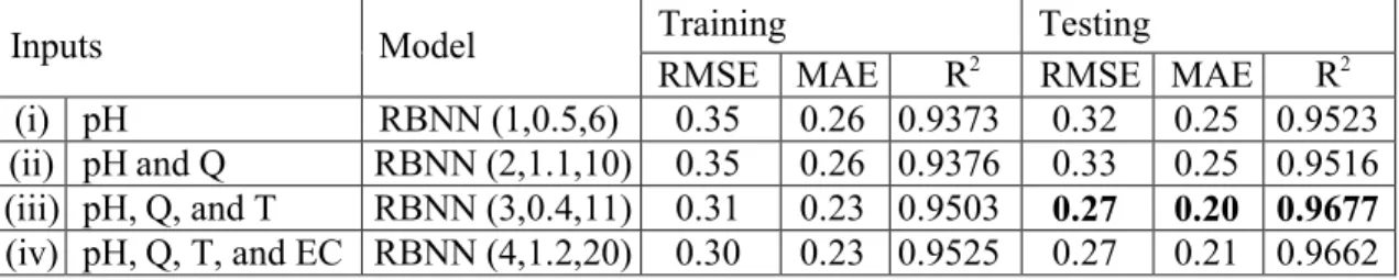
(i) pH RBNN (1,0.5,6) 0.35 0.26 0.9373 0.32 0.25 0.9523 (ii) pH and Q RBNN (2,1.1,10) 0.35 0.26 0.9376 0.33 0.25 0.9516 (iii) pH, Q, and T RBNN (3,0.4,11) 0.31 0.23 0.9503 0.27 0.20 0.9677
(iv) pH, Q, T, and EC RBNN (4,1.2,20) 0.30 0.23 0.9525 0.27 0.21 0.9662 For the comparison with MLP and RBNN models, the MLR models were also applied to the same data. The training and test results of the MLR models are given in Table 3. It is clear from this table that the MLR (4) model has the best accuracy.
Table 3 RMSE, MAE and R2values of the MLR models in training and test phases
Inputs Model Training Testing
RMSE MAE R2 RMSE MAE R2
(i) pH MLR (1) 0.33 0.26 0.9514 0.33 0.26 0.9514
(ii) pH and Q MLR (2) 0.33 0.26 0.9515 0.33 0.26 0.9515 (iii) pH, Q, and T MLR (3) 0.44 0.26 0.9517 0.44 0.26 0.9517 (iv) pH, Q, T, and EC MLR (4) 0.32 0.25 0.9542 0.32 0.25 0.9542
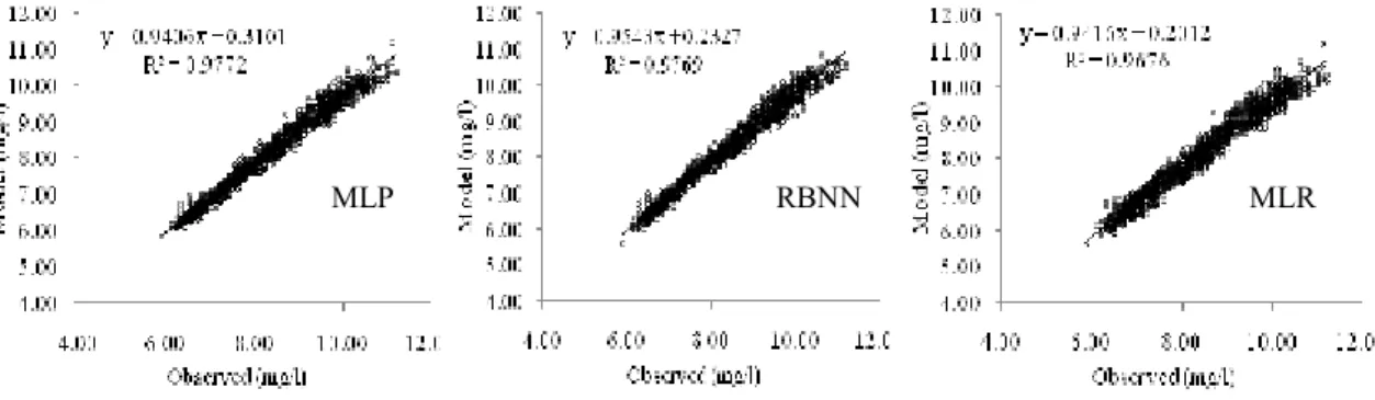
The validation accuracy of the optimal MLP (4,1,1), RBNN (3,0.4,11) and MLR models are compared in Table 4. It can be obviously seen from this table that the RBNN model performs better than the MLP and MLR models. MLR model gave the worst estimates. The models are graphically compared in Figure 4 in the form of scatter plot. The fit line equations in this figure clearly show that the RBNN performs better than the MLP and MLR models.
Table 4 Comparison of MLP, RBNN and MLR models in validation phase
Inputs Model RMSE MAE R2
pH, Q, T, and EC MLP (4,1,1) 0.27 0.21 0.9772 pH, Q, and T RBNN (3,0.4,11) 0.24 0.19 0.9769
MLP RBNN MLR
Figure 4 The optimal MLP, RBNN and MLR models in validation phase
CONCLUSIONS
Modeling of water quality variables is a very important aspect in the analysis of any aquatic systems. The chemical, physical, and biological components of aquatic ecosystems are very complex and nonlinear. In recent years, computational–intelligence techniques such as neural networks, fuzzy logic, and combined neuro–fuzzy systems have become very effective tools to identification and modeling nonlinear systems. In this study ANN structure was designed, trained, and tested using the MATLAB Neural Network Toolbox. The ability of two different ANN techniques (MLP and RBNN) and MLR model for estimating daily DO concentration has been investigated in the study. Models were tested according to the RMSE, MAE and R2 criteria. Comparison of the results indicated that the MLP and RBNN performed better than the MLR models. RBNN (3,0.4,11) model with three inputs which are pH, Q, and T was found to be the best model in estimation of DO concentration. The results showed that the water quality parameters, temperature (T), discharge (Q) and pH are effective parameters to estimate DO concentration in this stream-gauging station.
Acknowledgments: The data used in this study were downloaded from the U.S. Geological Survey (USGS) web server. The authors would like to thank the staffs of the U.S. Geological Survey (USGS) who are associated with data observation, processing, and management of the U.S. Geological Survey (USGS) web sites.
REFERENCES
[1] WEP (1996). Lower Great Miami watershed enhancement program. Miami valley index. Available at: http://www.mvrpc.org/wq/wep.htm.
[2] SAFE Strategic assesment of Florida’s environmental (1995). Florida stream quality index, statewide summary. htpp://www.pepps.fsu.edu./safe/environ/sqw1.html.
[3] Official paper (2004). Official paper. Water pollution control regulations. Date: 31.12.2004, no. 25687 (in Turkish).
[4] EPA United State Environmental Protection Agency (1994). Water Quality Standards Handbook, 2nd ed. htpp://www.epa.gov/waterscience/standardshandbook.
[5] Savcı, M. (1999). Irrigation water quality and irrigation by saltly water. Turkey civil engineering XV. technical congress paper book. Ankara, 713-731.
[6] Chau, K., (2006). A review on integration of artificial intelligence into water quality modeling.Marine Pollut. Bull. 52, 726-733.
[7] Dogan, E., Sengorur, B., and Koklu, R., (2009). Modeling biological oxygen demand of the Melen River in Turkey using an artificial neural network technique. J. Environ. Manage. 90, 1229-1235.
[8] Akkoyunlu, A., Altun, H., and Cigizoglu, H.K., (2011). Depth integrated estimation of the lake dissolved oxygen (DO).ASCE.Doi:10.1061/(ASCE)/EE,1943-7870.0000376. [9] Singh, K.P., Basant, A, Malik, A., and Jain, G. (2009). Artificial neural network
modeling of the river water quality-A case study.Ecol. Modeling. 220, 888-895. [10] Palani, S., Liong, S.Y., and Tkalich, P., (2008). An ANN application for water quality
forecasting.Marine Pollution.Bull. 56, 1586-1597.
[11] Soyupak, S., Karaer, F., Gürbüz, H., Kivrak, E., Sentürk, E., and Yazici, A., (2003). A neural network-based approach for calculating dissolved oxygen profiles in reservoirs.
Neural Comput. Appl. 12, 166-172.
[12] Chaves, P., and Kojiri, T., (2007). Conceptual fuzzy neural network model for water quality simulation.Hydrol. Process. 21, 634-646.
[13] Kuo, J.T., Hsieh, M.H., Lung, W.S., She, N., (2007). Using artificial neural network for reservoir eutrophication prediction.Ecol. Model.200, 171-177.
[14] Ying, Z., Jun, N., Fuyi, C., and Liang, G., (2007). Water quality forecast through application of BP neural network at Yuquio reservoir.J.Zhejiang Univ. Sci. A 8, 1482-1487.
[15] Haykin, S. (1998). Neural Networks: A comprehensive foundation, 2nd edn. Prentice-Hall, Upper Saddle River, NJ, pp 26-32.
[16] Marquardt, D. (1963). An algorithm for least squares estimation of non-linear parameters.Journal of the Society Industiral and Applied Mathematics, 11:431-441. [17] Hagan MT., and Menhaj MB (1994). Training feed forward networks with the
Marquardt algorithm.IEEE Trans Neural Netw5(6):861-867.
[18] Kisi, O. (2004). Multi-layer perceptrons with Levenberg-Marquardt training algorithm for suspended sediment concentration prediction and estimation. Hydrol Sci J
49(6):1025-1040.
[19] Broomhead D., and Lowe D., (1988). Multivariable functional interpolation and adaptive networks.Complex Syst2(6):321-355.
[20] Poggio, T., and Girosi, F. (1990). Regularization algorithms for learning that are equivalent to multilayer networks.Science, 2247, 978-982.
[21] Lee GC., and Chang SH (2003). Radial basis neural network function Networks applied to DNBR calculation in digital core protection systems. Ann Nucl Energy