HAL Id: hal-02153853
https://hal.archives-ouvertes.fr/hal-02153853v2
Preprint submitted on 1 Jul 2019
HAL is a multi-disciplinary open access archive for the deposit and dissemination of sci-entific research documents, whether they are pub-lished or not. The documents may come from teaching and research institutions in France or abroad, or from public or private research centers.
L’archive ouverte pluridisciplinaire HAL, est destinée au dépôt et à la diffusion de documents scientifiques de niveau recherche, publiés ou non, émanant des établissements d’enseignement et de recherche français ou étrangers, des laboratoires publics ou privés.
Increasing Returns, Balanced-Budget Rules, and
Aggregate Fluctuations
Maxime Menuet, Alexandru Minea, Patrick Villieu
To cite this version:
Maxime Menuet, Alexandru Minea, Patrick Villieu. Increasing Returns, Balanced-Budget Rules, and Aggregate Fluctuations. 2019. �hal-02153853v2�
Increasing Returns, Balanced-Budget Rules,
and Aggregate Fluctuations
Maxime Menueta, Alexandru Mineab,1, Patrick Villieua aUniv. Orl´eans, CNRS, LEO, UMR 7322, FA45067, Orl´eans, France
bSchool of Economics & CERDI, Universit´e d’Auvergne Department of Economics, Carleton University, Ottawa, Canada
Abstract
This paper examines the conditions needed for equilibrium (in)determinacy in growth models characterized by perfect competition and a balanced-budget rule (BBR). Contrary to the literature that assumes zero public debt, we build an endogenous growth model with a generalized BBR authorizing a constant positive debt level. We show that the emergence of aggregate instability dramatically depends on the dynamics of the debt-to-GDP ratio and the strength of social labor externalities. If the labor demand is positively sloped and steeper than the labor supply, two reachable balanced-growth paths appear – a no growth trap, and a positive growth solution – that gives birth to both local and global indeterminacy, hence aggregate instability driven by self-fulfilling beliefs (sunspots). In addition, we show that a fiscal rule such that the tax rate strongly responds to public-debt increases can remove the no-growth trap, and secure positive long-run growth. JEL classification: E62; O41
Keywords: Endogenous growth; indeterminacy; balanced-budget rules
1. Introduction
The emergence of indeterminacy in growth models characterized by perfect competi-tion and a balanced-budget rule have received much attencompeti-tion in macroeconomic theory. In a seminal paper, Schmitt-Groh´e and Uribe (1997, henceforth SU) first show that the steady state of a neoclassical growth model can be locally undetermined, giving rise to belief-driven fluctuations (sunspots). In their setup, public spending is exogenous, and the adjustment variable in the government’s budget constraint is the tax rate on labor income.
Many recent contributions pursued the SU’s research program by assuming a public spending-based adjustment with a fixed tax rate. Indeterminacy then crucially depends
1Corresponding author: [email protected].
We are particularly indebted to Jess Benhabib, Gareth Myles, and Alain Venditti for extensive excellent comments and suggestions on a previous version. Usual disclaimers apply.
on the usefulness of government expenditures. If public spending exerts some positive externality in households’ utility function or in the production function, the steady state can remain undetermined.2 However, if government expenditures are “wasteful”, Guo
and Harrison (2004, henceforth GH) showed that the steady state exhibits saddle-path stability, thus removing indeterminacy. Indeed, in an exogenous growth setup with a fixed tax rate on labor, the decreasing marginal products of capital and labor prevent agents expectations from becoming self-fulfilling.
The present paper explores the conditions for indeterminacy to appear in an endoge-nous growth framework, with other assumptions similar to SU and GH (in particular: a continuous-time one-sector model with endogenous labor, an additive utility function, and a balanced-budget rule, hereafter BBR). In this setup, we introduce two important ingredients. First, based on the seminal contribution of Benhabib and Farmer (1994), the aggregate production function exhibits increasing return-to-scale. With endogenous growth, the total factor productivity depends on the economy-wide levels of capital and labor through external effects in the production process (in the next section we detail several arguments that explain why labor social returns can be higher than the individual-firm returns). This can generate high labor externalities that produce nonlinearities in the dynamics of the consumption-to-capital ratio. Second, thanks to endogenous growth, our setup is characterized by non-trivial dynamics of the debt-to-capital ratio, even under the BBR. Effectively, the BBR defines situations such that public debt is constant, but non necessarily zero.3 When the rate of economic growth is endogenously determined, such situations are consistent with either (i) a permanent positive growth giving rise to a (asymptotical) zero debt ratio in the long run, or (ii) a positive long-run debt ratio associated with the (asymptotical) disappearance of growth. This creates the possibility of multiple perfect-foresight balanced-growth paths (BGP).
Our results are as follows.
First, we show that, in an endogenous growth framework, wasteful government spend-ing can be associated to both local and global indeterminacy. This findspend-ing conflicts with the GH’s determinacy result established in a neoclassical growth model.
Second, we exhibit two regimes depending on the strength of social labor externalities.
2See, e.g., Futagami and Mino (1995); Cazzavillan (1996); Palivos et al. (2003); Chen (2006); Guo
and Harrison(2008);Chen and Guo(2013a,b), among others. Capital-labor substitution or consumption externalities can also generate indeterminacy in exogenous growth model, see, e.g. Alonso-Carrera et al.
(2008) andWong and Yip(2010).
3A number of recent works have shown that endogenous growth setups provide a useful framework
for analyzing the effects of a continuous grow of public debt in the long run; see, e.g., Minea and Villieu
(2012);Nishimura et al.(2015a);Boucekkine et al.(2015);Nishimura et al.(2015b);Menuet et al.(2018). Albeit we focus here on BBR regimes, to make our results easily comparable to GH, our model can be extended to deficit rules without qualitative changes (see our extension in subsection 4.2).
If externalities are low, only one steady state, characterized by positive growth, can be reached in the long run, and the model is locally and globally well-determined. In con-trast, in the presence of high externalities, two reachable long-run equilibria emerge: a no-growth trap with positive debt ratio, and a positive-no-growth BGP with zero debt, the lat-ter being undelat-termined. Our model is then characlat-terized by aggregate instability, namely local and global indeterminacy, driven by self-fulfilling beliefs (sunspot). Importantly, the condition for indeterminacy to appear is the same as in Benhabib and Farmer (1994), namely the labor demand must be positively sloped and steeper than the labor supply. However, our aggregate-instability result covers a broader class of mechanisms than in
Benhabib and Farmer (1994), because it may rely on local and global indeterminacy. Third, we extend our model, and consider a fiscal rule such that the tax rate strongly responds to public-debt increases. Even if global indeterminacy remains (because two positive BGPs are feasible), this tax rule can remove the no-growth trap, and secure positive long-run growth. Indeed, a sufficient tax-increase can generate a positive re-lationship between government spending and public debt, such that the debt-to-output ratio follows an unstable trajectory around the no-growth trap.
Our paper complements the fast-growing literature on indeterminacy in endogenous growth models.4 Starting from the seminal paper of Matsuyama (1991), local and global indeterminacy are mainly studied in two (or multiple)-sectors models,5 or in the context of a public capital externality (productive or welfare-enhancing public spending).
In contrast, in our simple one-sector model with wasteful public spending, indetermi-nacy comes from two mechanisms. First, the presence of public debt is needed for mul-tiplicity to arise.6 Indeed, under a BBR, the non-trivial dynamics of the debt-to-capital ratio give rise to complex interactions between the government’s budget constraint and the households’ saving behavior. Second, following Benhabib and Farmer (1994);Farmer and Guo(1994), strong increasing returns-to-scale are needed for indeterminacy to emerge. In this case, labor supply and output positively depend on consumption, which can generate indeterminacy.
On the methodological side, the switch from exogenous to endogenous growth settings has two implications. One the one hand, the SU’s and GH’s conclusions regarding the determinacy of the steady state when the adjustment is based on wasteful public spending are dramatically changed.7 On the other hand, in an endogenous growth framework, the
4See the surveys of Benhabib and Farmer (1999), chap. 6, or Mino et al. (2008) regarding the local
indeterminacy.
5See, e.g.,Benhabib et al.(2000);Drugeon and Venditti(2001);Brito and Venditti(2010);Nishimura
et al.(2013), among others.
6Some papers have shown that endogenous growth models with public debt generate two steady-states
(Minea and Villieu,2012;Nishimura et al.,2015a;Menuet et al., 2018).
7This issue has already been raised in the literature on progressive taxation, where neoclassical growth
Benhabib and Farmer(1994)’s indeterminacy condition is more realistic. Effectively, since the total factor productivity is endogenous, strongly increasing returns-to-scale (relative to all inputs) are reachable even if the production function exhibits constant returns-to-scale relative to reproducible factors.
In terms of policy implications, our results suggest that a public spending-based ad-justment, together with a balanced-budget rule, can lead to an indeterminacy driven by agents’ animal spirits. Then, the economy can converge to a no-growth trap in the long run. However, we show that this undesirable feature can be removed if the government adopts a fiscal rule such that the tax rate strongly responds to the increase in public debt. This result illustrates the so-called concept of “fiscal space”, whereby public debt sustainability is ensured only if the primary budget surplus positively reacts to the debt burden (Ostry et al.,2015).
The remainder of the paper is organized as follows. Section 2 presents the model, section 3 studies a simple case without public debt, section 4 computes the steady states in the general case with public debt, section 5 deals with local and global dynamics, section 6 extends the model to a time-varying tax rate, and section 7 concludes.
2. The model
We consider a simple continuous-time endogenous-growth model with N representa-tive individuals, and a government. Each representarepresenta-tive agent consists of a household and a competitive firm. All agents are infinitely-lived and have perfect foresights. Popu-lation remains fixed over time, and we denote individual quantities by lower case letters, and aggregate quantities by corresponding upper case letters, namely X = N x, for all variable X.
2.1. Households
The representative household starts at the initial period with a positive stock of capital (k0), and chooses the path of consumption {ct}t≥0, hours worked {lt}t≥0, and capital {kt}t>0 to maximize the present discounted value of its lifetime utility, which is assumed to be separable U = ∞ ! 0 e−ρt " log(ct)− χ 1 +εl 1+ε t # dt, (1)
where ρ ∈ (0,1) is the subjective discount rate, ε ≥ 0 is the constant elasticity of intertemporal substitution in labour, and χ>0 is a scale parameter.8
2013b) are associated with local indeterminacy.
Households use their income (wtlt, wherewt is the hourly wage rate), to consume (ct), and to invest in capital ( ˙kt) and in government bonds (dt), which return respectively qt and rt (the real interest rate). They pay taxes on the wage income (τwtlt, where τ is the exogenous wage tax rate), hence the following budget constraint
˙
kt+ ˙dt =rtdt+qtkt+ (1−τ)wtlt−ct. (2) Defining by λt the costate variable of the current Hamiltonian, the first-order condi-tions for the maximization of the household’s programme (with rt = qt in competitive equilibrium) are 1/ct =λt, (3) χltε=λt(1−τ)wt, and ˙ λt= (ρ−rt)λt.
These conditions give rise to the familiar Keynes-Ramsey rule ˙
ct ct
=rt−ρ, (4)
and to the static relation
χlεt = (1−τ)wt/ct. (5)
Eq. (5) means that, at each periodt, the marginal gain of hours worked (the net real wage (1−τ)wt, expressed in terms of marginal utility of consumption 1/ct) just equals the marginal cost (χlε
t).
Finally, the optimal path of consumption has to verify the set of transversality con-ditions lim t→+∞{exp(−ρt) u ′(ct)k t}= 0 and lim t→+∞{exp(−ρt) u ′(ct)d t}= 0, ensuring that lifetime utility U is bounded.
2.2. Firms
The representative firm produces output (yt) using private capital (kt) and labor (lt), augmented by an externality that depends on the aggregate levels of both capital and labor, namely yt = ˜Aktα(lt)1−αK
θ1
t Lθt2, where ˜A >0 is a scale parameter, α ∈(0,1) is the elasticity of output to private capital, and θ1 and θ2 are positive parameters that reflect the externalities. This specification closely follows Benhabib and Farmer (1994).
As usual, the production function exhibits constant returns-to-scale at the individual level. Thus, the first-order conditions for profit maximization (relative to private factors)
are rt=α yt kt , (6) wt = (1−α) yt lt . (7)
To obtain an endogenous growth path, we consider constant capital returns (θ1 = 1−α). Thus, in the symmetric equilibrium (Lt=N lt, and Kt =N kt) we obtain
Yt= ˜AKtLφt, (8) where φ:= 1−α+θ2.
In our model, labor social returns (φ) can be higher than the individual-firm returns (1−α), thanks to the externalities. Three main arguments can sustain such a frame-work, and explain the presence of the parameter θ2 ≥0: (i) knowledge externalities, (ii) agglomeration effects, and (iii) thick market externalities.
(i) First, following Romer (1986), one can consider that the output of an individual firm (yt) is obtained with physical and human capital (ht), the latter being produced with raw labor (or training activity) lt and the economy-wide stock of knowledge Xt, namely ht = Xtlt. Using a constant returns-to-scale technology, we thus have yt = ˜Aktαh1t−α. Suppose that knowledge is produced by a simple Cobb-Douglas technology depending on the aggregate levels of physical and human capital: Xt=HtβKt1−β, where β ∈(0,1) is a measure of human capital efficiency in the accumulation of knowledge. At the aggregate level, we then obtain Ht = KtLt1/(1−β).9 Hence, the aggregate production function is Yt = ˜AKtLφt, with φ = (1−α)/(1−β). Then, parameter θ2 is endogenously determined as θ2 =β(1−α)/(1−β)≥0.
(ii) Second, agglomeration effects can justify Eq. (8). For example, urban production externalities are likely to produce spillovers among producers in areas with a high den-sity of economic activity (Krugman, 1991). In the presence of high localized knowledge spillovers, firms tend to locate in the proximity of each other to capitalize on the aggre-gate knowledge stock, namely, e.g., ytj = ˜Aktα(ltejt)1−α, where ejt is the agglomeration externality in location j in time t. Following Lucas and Rossi-Hansberg (2002), ejt mea-sures the mass of firm in location j, namely, if the size of the agglomeration is assumed to be one, etj =
$1
0 ytjdj. In symmetric equilibrium, ytj = yt for any j, the aggregate production function becomes Yt = ˜AKtLt(1−α)/α. In this case, φ = (1−α)/α, and the
9Human capital externalities, i.e. the mere idea that your coworkers’ human capital makes you more
productive, are well documented in the empirical literature (see, e.g. Rauch,1993; Moretti,2004, who provide robust support for large human capital externalities). Note that, since knowledge is produced with both human and physical capital, labor externalities can be very high in the aggregate production function (8). Alternative models of endogenous growth, based on the Lucas(1988)’s archetype, consider the formation of human capital through individual training decisions that compete with productive activities. See alsoBond et al.(1996).
corresponding value obtained for θ2 is now θ2 = (1−α)2/α≥0.
(iii) Third, another source of labor externalities may be derived from “thick market externalities” (Diamond, 1982), namely a friction related to firm-to-firm transactions. This externality is based on the increasing returns-to-scale matching technology in labor markets, so that search costs are lower as the size of the labor market increases.10 The adoption of an innovation can also generate a positive externality on other traders, thus creating strategic complementarities between the innovation decisions of different firms (Acemoglu, 1997). Altogether, these arguments support the presence of labor returns, which are potentially higher from the social perspective than from the firm-specific level (i.e. φ>1−α).
2.3. The government
The government provides public expenditures Gt, levies taxes, and borrows from households. The fiscal deficit is financed by issuing debt ( ˙Dt), hence, the following budget constraint
˙
Dt=rtDt+Gt−τwtLt. (9) With a fixed tax rate (τ), there are two potential policy instruments in Eq. (9): public debt (Dt), and public spending (Gt). Following GH, we consider endogenous public spending under a balanced-budget rule (BBR). Without public debt, this rule is simplyGt=τwtLt. However, with public debt, the BBR requires ˙Dt= 0 ⇒Dt =D0,∀t, namely
Gt=τwtLt−rtD0. (10) Hence; the BBR is consistent with a constant (not necessarily zero) public debt level. We denote this relation as a generalized BBR. Such a situation characterizes almost all countries under BBR, because, at the date they adopt the BBR, countries most often experiment high public debt (D0 > 0). This feature has crucial implications, since our model can exhibit complex dynamics of the public debtratio(D0/Yt), even in the presence of a BBR.11
2.4. Equilibrium
To find endogenous growth solutions, we deflate all growing variables by the capital stock to obtain long-run stationary ratios, namely (we henceforth omit time indexes) yk:=Y /K, ck :=C/K and dk :=D0/K.
10FollowingHall(1993) “the overall technology of an industry with a thick-market externality will have
increasing returns even though each firm has constant returns” (p. 94). Caballero and Lyons (1992) found empirical support for external increasing returns to scale, which can be interpreted as thick-market externalities. For a growth model with endogenous human capital and labor participation, see
Chen et al.(2011).
11Our results hold with a more general set of deficit rules, such as, e.g., ˙D
t = θYt, where θ is the
The optimal consumption behaviour is, from (4) and (6), ˙
C
C =αyk−ρ, (11)
while the path of the capital stock is given by the goods market equilibrium ˙
K
K =yk−ck−gk. (12) From (6) and (10), the public spending ratio is defined as
gk = [τ(1−α)−αdk]yk, (13) and from (5) and (7) we obtain the output ratio
yk =Acψk, (14)
where ψ :=φ/(φ−1−ε), andA:= ˜A%A˜(1 χ
−α)(1−τ)Nε &ψ
>0.
The relationship between the consumption and the output ratios crucially depends on the sign of ψ, which is related to the strength of labor social returns. Effectively, the aggregate production function can exhibit increasing labor return if labor market exter-nalities are high enough (i.e. θ2 >α ⇒ φ > 1). Consequently, ψ can be either positive – and higher than one –12 or negative, thereby depicting an increasing or a decreasing relation between the consumption and the output ratios.
The reduced-form of the model is obtained from Eqs. (6)-(7)-(10)–(11)-(12)-(13), namely, using ¯d:= (1−τ)(1−α)∈(0,1), ⎧ ⎪ ⎪ ⎨ ⎪ ⎪ ⎩ ˙ ck ck =ck−ρ−( ¯d+αdk)yk, ˙ dk = [ck−( ¯d+α+αdk)yk]dk. (15)
As it should clearly appear, the presence of a constant positive public debt level in the generalized BBR (10) generates non trivial dynamics of the public-debt ratio (dk) in the reduced form (15). In an exogenous growth context, the generalized BBR (10) does not fundamentally change the dynamic properties of the steady state compared with a simple BBR without debt, because the steady-state is unique and well determined, just as in GH (see Appendix A). With endogenous growth, in contrast, the generalized BBR, if associated to strong increasing returns in the production function, can produce multiple
perfect-foresight BGPs with possible local and global indeterminacy, as we will see. We determine the steady-state solutions of the model in section 4, and analyze local and global dynamics in section 5. Beforehand, to isolate the specific role of increasing returns and provide some intuition on the underlying mechanisms of the model, section 3 presents a simple special case without public debt.
3. A preliminary analysis: the case without public debt
Without public debt (dk = ˙dk = 0), the BBR simply writes Gt = τwtLt, and, using (13), the reduced-form of the model (15) boils down to a unique equation
˙ ck ck
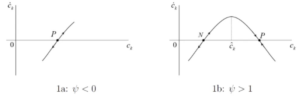
=ck−ρ−dAc¯ ψk =:Ψ(ck), (16) such that the long-run consumption ratio is defined by the implicit relation Ψ(ck) = 0.
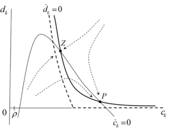
If ψ < 0, Ψ(·) is continuously increasing, hence the existence of one unique positive solution (point P in Figure 1a). Moreover, as Ψ′(·)> 0, this solution is unstable. Since
the consumption ratio ck is a jump variable, the steady state is well-determined (the economy initially jumps at point P).
However, if ψ > 1, Ψ(·) takes a maximum at point ˆck := (ψdA¯ )1/(1−ψ), such that Ψ′(ˆck) = 0 and Ψ′′(ˆck) < 0. Thus, there are two positive long-run solutions, namely cN
k and cPk, which correspond respectively to points N and P in Figure 1b. Note that cN
k is associated to a negative growth rate in steady state, while cPk is associated to a positive BGP, under the mild condition that the discount rate is small enough, i.e.
ρ<ρ¯:=αA[A(α+ ¯d)]ψ/(1−ψ), that we assume throughout the paper (as we will see below, this condition ensures the existence of BGPs).13 Clearly, as Ψ′(cN
k)>0 and Ψ′(cPk)<0, and ck being a jump variable, the negative growth solution is unstable (well determined) while the positive growth solution is saddle-point stable (locally undetermined).
Figure 1: Phase portrait in the no-debt case
13In the long run, the growth rate isγ=αAcψ
k−ρ. Thus, sinceψ>1,γ>0⇔ck>¯ck:= (ρ/αA)1/ψ.
Yet,Ψ(¯ck)>0⇔ρ<ρ¯. Consequently, ifρ<ρ¯, there are two positive solutions: cNk <c¯k andcPk >¯ck;
Consequently, in the case ψ >1 the economy is characterized by aggregate instability that relies both on local and global indeterminacy. Effectively, two perfect-foresight BGPs can be reached in the long-run (global indeterminacy), and the transition path in the neighborhood of P is subject to sunspot equilibria (local indeterminacy). If ψ <0, in contrast, the BGP is unique and there is no aggregate instability, as in GH.
The existence of these two regimes crucially rests on the relation between the con-sumption and the output ratios in Eq. (14), which can be either positive or negative. This property comes from the labor market equilibrium (5). As consumption increases, its marginal utility decreases, thus inducing the representative household to substitute leisure for working hours, because the shadow price of labor (λ, see Eq. 3) declines. The higher the elasticity (ε) the stronger the reduction in worked hours. To restore equi-librium, the real wage must rise. In the first order condition for profit maximization (7), this arises only if the average product of labor (Y /L) goes up, namely if φ > 1. Therefore, as the consumption ratio jumps up, households are induced to increase labor supply only if the real wage responds strongly enough to compensate the disutility of work (φ > 1 +ε ⇒ ψ > 1); hence a rise in the output ratio. In the opposite case (φ<1 +ε⇒ψ <0), labor supply decreases and the output ratio goes down.
The intuition of this analysis is close to Benhabib and Farmer (1994), but in the context of endogenous growth. By injecting the real wage rate (7) into the first-order condition for the optimal choice of labor (5), we obtain
χ(Ct/Kt)(Lt/N)ε =A(1−τ)(1−α)Lφt−1. By taking logarithms, the labor supply curve is
˜
wt= cst1+ ln(Ct/Kt) +εL˜t, and the labor demand curve is
˜
wt= cst2+ (φ−1) ˜Lt.
where ˜wt is the logarithm of the real wage per capital, and ˜Lt the logarithm of the real labor (with the two constants cst1 := ln(χ/Nε) and cst2 := ln(A(1−τ)(1−α))). Thus, labor demand is decreasing with real wage if and only if φ<1. In this case, the higher the consumption ratio, the higher the employment and the output on the BGP. In contrast, if φ>1, labor demand is, in equilibrium, positively-sloped.
Figure 2 examines the effects of a rise in the consumption ratio in the case of a positively-sloped labor demand (φ > 1). If ε < φ −1 (i.e. ψ > 0), the slope of the demand curve (φ−1) exceeds the slope of the supply curve (ε), so that an increase in the consumption-to-capital ratio rises employment, output, and the real wage (see Figure 2a). In contrast, if ε>φ−1 (i.e. ψ <0), a rise in the consumption ratio is accompanied
by a decline in employment and output on the BGP (Figure 2b illustrates this case for 1<φ <1 +ε). ˜ wt ˜ Lt ck 0 labor demand labor supply • • a. If ε <φ−1 ˜ wt ˜ Lt ck 0 labor demand labor supply • • b. If ε >φ−1
Figure 2: Effect of a rise in the consumption ratio (positively sloped labor demand)
Importantly, the condition ψ > 0 corresponds to the Benhabib and Farmer (1994)’s criterion to generate local indeterminacy in a neoclassical growth model with increasing returns. In our model too, a necessary condition for aggregate instability to emerge is that the real wage is increasing with the employment level.
Two points deserve particular attention. First, although this criterion has been chal-lenged from an empirical perspective,14 in our endogenous growth setup the condition
φ>1 +ε is realistic. Effectively, considering the knowledge-externality interpretation of the model (with the firm-specific and knowledge production functions yt= ˜Aktα(Xtlt)1−α and Xt = HtβK
1−β
t , respectively), this condition is verified for, e.g., β > α if the Frisch elasticity of labor supply is infinite (ε= 0), as usual in business cycle literature (see, e.g. SGU). It looks as quite reasonable to suppose that the elasticity of knowledge to human capital is greater than the physical capital share in output (around α = 1/3).
Second, in our model, the criterion φ >1 +ε is a necessary and sufficient condition to ensure not only local but also global indeterminacy. Nevertheless, at this stage our
14To this day, there is no agreement in the literature on the degree of aggregate returns-to-scale. The
first papers based on simple linear regressions in macro models highlighted quantitatively significant increasing returns-to-scale in U.S. manufacturing (Caballero and Lyons, 1992;Hall, 1993). Subsequent works challenged this view (Basu and Fernald,1997;Burnside,1996), suggesting that the U.S. manufac-turing industry displays constant returns with no external effects (while there is significant heterogeneity across industries). However, more recent papers found that, contrary to many previous results, US economic growth has been driven by increasing returns-to-scale rather than technical progress ( Diew-ert and Fox, 2008). As pointed out by Hall (1993), this controversy can be related to the difficulty of identifying separately the returns to scale and TFP growth. In neoclassical (exogenous) growth models, TPF is the engine of growth, and the measure of returns-to-scale must be insolated from the measure of technical progress. In our endogenous growth setting, TFP is endogenous, and the production function exhibits constant returns-to-scale relative to reproducible factors, i.e. when labor is measured in efficient units (yt = ˜Akαth1t−α). This does not preclude the existence of large increasing returns-to-scale at the
setup exhibits two shortcomings. Effectively, the absence of transitory dynamics and the presence of a negative long-run BGP are questionable, both on the empirical side and from an endogenous growth perspective. The following sections address these issues, by considering the general version of the model with public debt.
4. The general case with public debt
In the general model, we define a BGP as a path on which consumption, capital, and output grow at the same (endogenous) rate, namely: ˙ck = ˙dk = 0 in (15). Thus, for any steady-state i, we have: γi := ˙C/C = ˙K/K = ˙Y /Y, while the real interest rate (ri) is constant.
The long-run endogenous growth solutions can be described by two relations between ck and dk. The first one is the ˙ck = 0 locus, which comes from the Keynes-Ramsey relation (11) and the IS equilibrium (12)
ck−ρ= ( ¯d+αdk)yk. (17)
The second relation is the ˙dk= 0 locus, namely
γdk= 0, (18)
where γ := ( ¯d+α+αdk)yk−ck is the long-run growth rate. Eq. (18) means that either the long-run public debt is positive and the associated growth rate is zero (zero growth solution, such as dk >0 ⇒γ = 0), or the long-run growth rate is positive (or negative) with zero public debt (γ >(<)0⇒dk = 0).
4.1. Characterization of steady states
Steady-state solutions are obtained at the crossing-points of Eqs. (17) and (18). Theorem 1. If ρ<ρ¯, the long-run equilibria are characterized by the following regimes.
• Regime R1: ψ <0. There are one positive growth solution (point Q), and one zero growth solution (point Z).
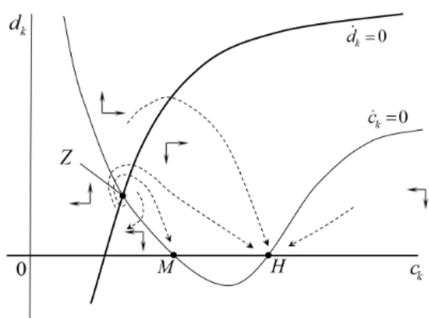
• RegimeR2: ψ >0. There are one negative solution (N), one positive solution (P), and one zero growth solution (point Z).
Proof. See Appendix B.
The multiplicity of steady states comes from the interaction between two nonlinear relationships linking the consumption and the debt ratios.
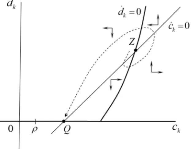
(i) The first relation stems from the government’s budget constraint ˙dk =−γdk = 0, which is verified either if dk = 0 (namely the x-axis in Figures 3 and 4) or if
γ = ( ¯d+α+αdk)yk(ck)−ck =ck[( ¯d+α+αdk)Acψk−1 −1] = 0.
Considering strictly-positive consumption ratios, this relation describes a monotonic association between ck and dk, which is positively-sloped if ψ < 0 (Figure 3), and negatively-sloped if ψ >0⇒ψ >1 (Figure 4).
(ii) The second relation is derived from the assumption of balanced-growth in the long run (namely ˙K/K = ˙C/C =γ), and corresponds to (17), withyk(ck) =Acψk.
If ψ < 0, an increase in the consumption ratio (ck) reduces the output ratio (yk), decreasing the RHS of (17). This generates a monotonic increasing relation between ck and dk (any positive deficit ratio is associated with one consumption ratio), as depicted in Figure 3. Therefore, there is only one consumption ratio that verifies dk = 0, hence the uniqueness of the non-zero growth solution (point Q).
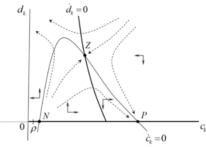
Figure 4: Phase portrait under regimeR2
In contrast, if ψ > 0 (see Figure 4), output increases with the consumption ratio, so that the two sides of Eq. (17) positively depend on ck, producing a non-monotonic relationship between ck and dk. In this case, any positive deficit ratio is associated with two consumption ratios. Consequently, two levels of ck verify dk = 0, hence the two non-zero growth solutions (points N and P).
4.2. Extension to permanent deficit rules
Although we focused so far on the BBR, our setup can be extended to the presence of continuous growth of public debt in the long run. Indeed, a number of recent papers have shown that endogenous growth is feasible with growing public debt in the steady state.15 With endogenous growth, output grows continuously along the BGP, allowing public debt to grow continuously (since the BGP is such that all variables grow at the same rate, the debt-to-output ratio is constant in the steady-state). Thus, contrary to exogenous growth models, the BBR is not necessarily required.
Hence, our model can be extended to deficits rules involving a constant deficit-to-output ratio θ≥0, such that16
˙
Dt=θYt. (19)
In this respect, the case θ = 0 amounts to our generalized BBR, which corresponds to a constant (but not necessarily zero) public debt.
15See, e.g.,Minea and Villieu(2012),Nishimura et al. (2015a),Nishimura et al.(2015b), andMenuet
et al.(2018) for an extension to money financing.
16This rule authorizes permanent deficits in the long run, which is consistent with OECD’s fiscal
positions (prior to the Great Recession, the average public deficit was about 2.5% of GDP from 1970 to 2005, namely θ = 0.025). One could also specify a deficit rule with a gradual adjustment path of the
With such a deficit rule, the reduced form of the model (15) must be amended as follows: (i) coefficient ¯d must be redefined as ¯d := (1−τ)(1−α)−θ, which is positive for small θ, and (ii) the debt to capital ratio now evolves according to
˙
dk =θyk+ [ck−( ¯d+α+αdk)yk]dk.
Consequently, the ˙ck= 0 locus (17) is unchanged, notwithstanding the redefinition of ¯
d, while the ˙dk = 0 locus (18) becomes now
θyk=γdk. (20)
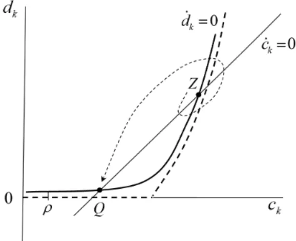
With small positive values of the deficit ratio (namely θ > 0), previous results are qualitatively unchanged, as show Figures 5 and 6, where the dashed- (resp. continuous-) bold lines describe the ˙dk = 0 locus in the case θ = 0 (resp. θ > 0). The major change is that the ˙dk = 0 locus is now a smooth curve that intersects twice the ˙ck = 0 locus, with point Z being now characterized by positive growth. Hence, the deficit rule θ >0 precludes negative and zero growth solutions in the steady state, because the long-run economic growth rate must be γ = ˙D/D = θY /D > 0 in equilibrium. For the same reason, the no-growth trap Z becomes now a low-growth trap, with (small) positive economic growth in equilibrium.
Figure 6: Phase portrait under regimeR2 (θ>0)
5. Analysis of dynamics
To study the behaviour of the model outside the steady-state, we first proceed to a local stability analysis, and then infer global dynamics. To simplify the exposition, we focus on the (generalized) BBR case (θ= 0).17
5.1. Local dynamics
By linearization in the neighborhood of steady-state i, i ∈ {N, P, Q, Z}, the system (15) behaves according to ( ˙ck,d˙k) =Ji(ck−cik, dk−dik), whereJi is the Jacobian matrix. The reduced-form includes one jump variable (the consumption ratio ck0) and one pre-determined variable (the public-debt ratio dk0, since the initial stocks of public debt D0 and private capital K0 are predetermined). Thus, for BGP i to be well determined, Ji must have two opposite-sign eigenvalues. Using (15), we compute
Ji = + CCi CDi DCi DDi , , where CCi =cik−( ¯d+αdik)ψyki, (21) CDi =−αcikyki, (22) DDi =−γi−αdikyki, (23) DCi = [1−Aψ(cik)ψ−1( ¯d+α+αdik)]dik. (24)
17The behaviour of the model is qualitatively unchanged with a deficit rule (θ>0), provided that the
Hence, the trace and the determinant of the Jacobian matrix are, respectively
Tr(Ji) =cik−( ¯d+αdik)ψyik−γi−αdikyki, (25) det(Ji) = −γi[ci
k−( ¯d+αdik)ψyki]−ψα2(yki)2dik. (26) The following theorem establishes the topological behaviour of each steady-state. Theorem 2. (Local Stability)
• In regime R1, Z is locally over-determined (unstable), and Q is locally determined (saddle-point stable).
• In regime R2, Z is locally determined (saddle-point), P is locally under-determined (stable), and N is locally over-determined (unstable).
Proof. See Appendix C.
The local stability of the zero growth solution (Z) is intuitive. Indeed, the sign of the determinant is the opposite of the sign of ψ. Therefore, in regime R2 (ψ > 0), the determinant is negative, hence the saddle-path property. In regime R1 (ψ <0), both the determinant and the trace are positive, hence the point Z is unstable.
As regards the non-zero growth solutions, we have dik = 0, namely DCi = 0, i ∈
{P, N, Q}. Consequently, the two eigenvalues (λi
1,λi2) are simply λ1i =DDi =−γi, and
λi
2 =CCi =cik−( ¯d+αdik)yki. In regime R1, point Q is associated to a positive growth rate (γQ > 0), and to CCQ > 0, hence the law of motion of consumption is unstable. Consequently, there is one negative and one positive eigenvalue, and Q is saddle-path stable. In regime R2, in contrast, the positive growth solution is such that CCP < 0. The law of motion of consumption is then stable, the two eigenvalues are negative, and P is locally undetermined (stable). At the negative growth solution (point N), however, we have CCN > 0, so that the two eigenvalues are positive, which makes N a locally over-determined (unstable) solution.
5.2. Global dynamics
Capitalizing on the local analysis, we can now evaluate the global dynamics. Accord-ing to theorem 2, we can distAccord-inguish two cases, dependAccord-ing on the sign of ψ.
Regime R1 – In this case, there are two steady states, but only the positive growth solution (Q) can be reached in the long run, as the zero growth trap (Z) is unstable. Indeed, for any predetermined debt ratio dk0 >0 the consumption ratiock0jumps to place the economy on the saddle-path that converges towards Q, which defines the unique long-run equilibrium (hence the absence of local or global indeterminacy). Consequently, in an endogenous growth setup with wasteful public spending, we find the GH’s determinacy result. However, this result does not hold in regime R2.
Regime R2 – As we have seen, there are three steady states: N is unstable, P is stable, and Z is saddle-path stable. Thus, the situation is characterized by local inde-terminacy (in the vicinity of the positive growth solution P), and global indeterminacy. Indeed, given a (predetermined) public debt ratio dk0 > 0, the initial consumption ra-tio can jump on the unique transira-tion path that converges towards Z, or on one of the multiple paths that converges towards P.
Consequently, the long-run equilibrium of the economy is subject to “animal spirits”, in the form of optimistic or pessimistic views of households at the initial time. The intuition is as follows. Let us suppose that, at the initial time, households expect a high consumption ratio and zero debt (point P) in steady state. Thus, the output ratio is expected to be high (as ψ > 0), which corresponds to high expected return of private capital. Then, at the initial time households are induced to save, leading to a self-fulfilling increase in economic growth. As a result, a belief-driven transitional path towards the the positive growth BGP (P) emerges.
In contrast, following the same mechanism, if high public debt and low return of saving are expected (along the Z BGP), households increase consumption and reduce investment at the initial time. This puts the economy on a self-fulfilling path towards the no-growth trap.
5.3. Discussion
In our model, multiplicity and indeterminacy result from two ingredients that closely interact: the dynamics of the public debt ratio, and the dynamics of the consumption ratio.
Regarding the first ingredient (ignoring negative growth situations), the BBR gen-erates two possible BGPs: a zero-growth solution with positive debt, and a zero debt solution with positive growth. Regarding the second ingredient, the determinacy of these two equilibria fundamentally depends on the effect of the consumption ratio in the IS equilibrium. As we have seen, in goods market, consumption increases the demand, while its effect on supply is more complex and depends on the labor market equilibrium through the sign of ψ.
If φ <1 +ε ⇒ψ <0, an increase in consumption negatively affects output, because households are induced to increase leisure. Consequently, a jump in the consumption ratio (ck) generates an excess demand in the goods market, producing an adverse effect on capital accumulation ( ˙K/K). This, leads to an increase in the path of the consumption ratio ( ˙ck/ck). Hence, the dynamics of ck is unstable, which explains the absence of indeterminacy.
If φ >1 +ε ⇒ψ >1, following a positive jump in consumption, the rise in the real wage is strong enough to overcome the disutility of labor, thereby labor supply and output increase. Interestingly, since ψ >1, this supply effect outweighs the increase in demand. As a result, the increase in the consumption ratio now generates a net excess supply in
the goods market. This boosts capital accumulation, which dampens the evolution of the consumption ratio ( ˙ck/ck is reduced). Hence, the dynamic of ck now becomes stable, giving birth to indeterminacy.
Roughly speaking, our model is in some sense “more stable” in the presence of strong labor externalities (i.e. ψ >0). This is consistent with theBenhabib and Farmer(1994)’s criterion to generate local indeterminacy of the perfect foresight equilibrium in a neo-classical growth framework. In our endogenous growth setup too, indeterminacy only emerges if ψ >0, but this indeterminacy presents a larger perspective than in Benhabib and Farmer (1994). Effectively, the caseψ >0 leads not only to local indeterminacy but also to a multiplicity of equilibria, leading to global indeterminacy. Indeed, for any initial value of the predetermined variable (the deficit ratio), the economy can reach either a positive growth solution, or an undesirable stagnation solution with zero growth, accord-ing to optimistic or pessimistic views of households. Given the undesirable possibility of the zero growth in the long-run, in the following section we relax the assumption of a constant tax rate, and attempt to characterize suitable fiscal rules that allow escaping the no-growth trap.
6. How to remove the no-growth trap? The case with a time-varying tax rate So far, we have considered a fixed tax rate. In this section, we extend our analysis to the case of a time-varying tax rate. To this end, we assume that the government is subject to a tax rule τ(dk), which belongs to the class of tax rules (T) requiring a higher tax rate as the public debt increases, namely T := {τ(dk)|τ(dk) ∈ C2,τ′(dk) ≥ 0}. To
assess whether such a fiscal rule allows removing the no-growth solution, we focus from now on regime R2.
It must be emphasised that, even if the tax rate is variable, the fiscal rule τ(dk) remains exogenously specified, and the adjustment variable in the government’s budget constraint remains wasteful public spending (gk), as in the previous sections.
The dynamic system (15) becomes
⎧ ⎪ ⎪ ⎨ ⎪ ⎪ ⎩ ˙ ck ck =ck−ρ−( ¯d(dk) +αdk)yk, ˙ dk = [ck−( ¯d(dk) +α+αdk)yk]dk, (27) where ¯d(dk) = (1−τ(dk))(1−α)∈(0,1).
With a time-varying tax rate, the relationship between public debt and public spend-ing is modified. Effectively, as gk = rdk +τ(dk)wtLt = [τ(dk)(1 −α)−αdk]yk, we can distinguish two cases following an increase in the debt ratio (dk).
(i) If τ′(dk) < τˆ := α/(1− α), the increase in the debt burden exceeds the new
qualitatively unchanged relative to the previous sections.
(ii) In contrast, if the fiscal rule generates high tax revenues, namely τ′(d
k) > τˆ, fiscal resources are strong enough to offset the increase in the debt burden, so that public expenditures rise, i.e. ∂gk/∂dk > 0. In this case, the dynamics of the model radically changes, as shows the following theorem.
Theorem 3. In regime R2 (i.e. ψ > 0), if τ′ > τˆ, there are critical levels ρˆ> 0 and ¯
τ0 >0, such that, if ρ<ρˆand τ(0) <τ¯0, there are two positive growth solutions (M and H), and one zero growth solution (Z).
Proof. See Appendix D.
The three equilibria still come from the interaction between two nonlinear relation-ships linking the consumption and the deficit ratios. If τ′ <τˆ, the situation is unchanged compared with the theorem 1. However, if τ′ >τˆ, two positive growth solutions emerge. Effectively, regarding the phase portrait (see Figure 7),18 there are two main differences relative to the previous section.
First, the stationary locus ˙ck= 0 now describes a U-shaped curve in the (ck, dk)-plane, and corresponds to
ck−ρ=ζ(dk)yk(ck), where ζ(dk) := ¯d(dk) +αdk. (28) As τ′(d
k)>ˆτ ⇔ ζ′(dk)<0, the relationship between dk and ck (in Figure 7) is inverted with respect to the preceding case under regime R2 (see Figure 4).
Second, the locus ˙dk/dk = 0 now describes an increasing curve, namely
γ = (ζ(dk) +α)yk(ck)−ck =ck[(ζ(dk) +α)cψk−1−1] = 0.
Asψ >1, an increase in ck rises the economic growth rate, hence a monotonic increasing relationship between ck and dk, becauseζ′(dk)<0.
Therefore, both loci are reversed relative to section 4. Effectively, if τ′ > τˆ, any
increase of the debt ratio (dk) rises public spending (gk) and thus reduces the economic growth rate (γ), whereas in section 4 with a constant tax rate (or more largely when
τ′ <τˆ), public spending and deficit were negatively related (see Eq. (13)). Consequently,
by implementing highly debt-sensitive tax rules, the relationship between public debt and economic growth reverses.
Figure 7: The phase portrait in regime R2 withτ′ >τˆ
Local dynamics. Let us now study the local stability when τ′ >τˆ. By diff erentiat-ing system (27), the components of the jacobian matrix Ji for steady-statei∈{H, M, Z}, are CCi =cik−ζ(dik)ψyki, (29) CDi =−ζ′(di k)cikyki, (30) DDi =−γi−ζ′(dik)dikyki, (31) DCi = [1−Aψ(cik)ψ−1(ζ(dik) +α)]dik. (32) Thus, the trace and the determinant of the Jacobian matrix are, respectively
Tr(Ji) = cik−ζ(dik)ψyik−γi −ζ′(dik)dikyki, (33) det(Ji) = −[cik−ζ(dik)ψyki]γi−αψζ′(dik)(yki)2dik, (34) and the following theorem characterizes the topological behaviour of each BGP.
Theorem 4. The zero-growth solution (Z) is unstable, the medium-growth solution (M) is saddle-path stable, and the high-growth solution (H) is stable.
Proof. See Appendix F.
The intuition driving the local behaviour of the positive growth solutions is the same as previously in regime R2. At pointsM and H, the two eigenvalues are: λi1 =DDi =−γi, and λi
2 = CCi = cik−ζ(0)ψyk. For ψ > 0, the medium-growth equilibrium M is such thatCCM >0, hence the law of motion of consumption is unstable. Consequently, there is one negative and one positive eigenvalue, and M is saddle-path stable. In contrast, the point H is such that CCH < 0. The law of motion of consumption is then stable, the two eigenvalues are negative, and H is locally undetermined (stable).
The heart of the mechanism that makes the zero-growth solution unstable is related to the relationship between public debt and public spending (∂gk/∂dk). As discussed above, we can distinguish two cases.
(i) If this relation is negatively-sloped (τ′ < τˆ), any increase in the public debt
ra-tio produces a higher net-of-taxes debt burden that requires a cut in public spending. This cut, in turn, generates a higher rate of capital accumulation in the goods market equilibrium, such that the debt-to-output ratio will decrease. Hence the stability of the debt path, which leads to the saddle-path property of the no-growth solution Z, as in the previous section.
(ii) In the case of a positively-sloped relation (τ′ > τˆ), however, the increase of the debt ratio generates enough fiscal resources too increase public spending despite the BBR. Consequently, the rate of capital accumulation falls in goods market equilibrium, and the debt-to-output ratio undertakes an unstable trajectory. As a result, the no-growth solution becomes unstable.
Global dynamics. If τ′ > ˆτ, the economy is characterized by both local
indeter-minacy (in the vicinity of the high growth solution H) and global indeterminacy. For a given (predetermined) public debt ratio dk0 >0, the initial consumption ratio can jump on the unique transition path that converges towards the medium-growth equilibrium (M), or on one of the multiple paths that converge towards H.
The main interest of a varying tax rate is that the economy cannot experiment the no-growth trap in the long run, provided that τ′ >τˆ. This analysis points out the need for indebted countries to implement stringent fiscal rules in order to make tolerable their public finance stance. This feature is consistent with the concept of the “fiscal space”, whereby public debt sustainability is ensured only if the primary budget surplus positively reacts to the debt burden (Ostry et al., 2015). As outlined by the proponents of fiscal space, the adjustment of the primary surplus can be made difficult given the presence of some social resistance to tax-increases, notably in a context of high debt. Therefore, the case with τ′ < τˆ reflects a narrow fiscal space, while the case τ′ > τˆ can be associated
to a large fiscal space. In these lines, our model reveals that the no-growth trap can be removed only if the fiscal space is large enough.19 However, as in the previous section, global indeterminacy remains and raises a similar selection problem, since the economy can converge towards different positive growth solutions.
7. Concluding remarks
This paper shows that local and global indeterminacy can appear in a one-sector en-dogenous growth model, when wasteful public expenditures adjust to the government’s
19A related analysis in a two-period game theoretic approach with tax policy becoming procyclical at
budget constraint. This result contrasts with usual findings in neoclassical (exogenous) growth models, showing that indeterminacy can emerge only with a tax-based adjuste-ment (Schmitt-Groh´e and Uribe, 1997), or when public expenditures are useful, i.e. pro-duce utility services and/or productive externalities (see, e.g. Guo and Harrison, 2008). Therefore, endogenous growth models can reverse results obtained in exogenous growth setups, as in Guo and Harrison (2004).
Fundamentally, this result comes from the nature of the BBR, which is consistent with non trivial dynamics of the debt ratio when considering endogenous growth. In our framework, ignoring negative growth solutions in steady-state, two admissible long-run equilibria emerges: a zero-growth BGP with positive debt, and a positive-growth BGP with zero debt. Both BGPs can be reached, as the stability analysis does not allow selecting a unique equilibrium.
However, a fiscal rule such that the tax rate strongly responds to public-debt in-creases can remove the no-growth trap, and secure positive long-run growth (even if indeterminacy remains, because two positive BGPs are feasible). This analysis calls for implementing tight tax policies in indebted countries,
This paper can be extended in several directions. For example, it would be worthwhile to examine alternative fiscal rules (see, e.g. Combes et al.,2017), or to introduce the case for money-financing (Menuet et al., 2018). In addition, possible extensions would study the robustness of our theoretical results, as the specification of non-separable preferences, progressive endogenous taxes, or useful public spending. We plan to pursue these research projects in the future.
References
Acemoglu, D., 1997. Training and innovation in an imperfect labour market. The Review of Economic Studies 64, 445–464.
Alonso-Carrera, J., Caball, J., Raurich, X., 2008. Can consumption spillovers be a source of equilibrium indeterminacy? Journal of Economic Dynamics and Control 32, 2883–2902.
Basu, S., Fernald, J.G., 1997. Returns to scale in US production: Estimates and implications. Journal of Political Economy 105, 249–283.
Benhabib, J., Farmer, R., 1994. Indeterminacy and increasing returns. Journal of Economic Theory 63, 19–41.
Benhabib, J., Farmer, R., 1999. Indeterminacy and sunspots in macroeconomics, in: Taylor, J., Wood-ford, M. (Eds.), Handbook of Macroeconomics. North Holland Publishing Co., Amsterdam, pp. 387– 448.
Benhabib, J., Meng, Q., Nishimura, K., 2000. Indeterminacy under constant returns to scale in multi-sector economies. Econometrica 68, 1541–1548.
Bond, E., Wang, P., Yip, C., 1996. A general two-sector model of endogenous growth with human and physical capital: balanced growth and transitional dynamics. Journal of Economic Theory 69, 149–173.
Boucekkine, R., Nishimura, K., Venditti, A., 2015. Introduction to financial frictions and debt con-straints. Journal of Mathematical Economics 61, 271–275.
Brito, P., Venditti, A., 2010. Local and global indeterminacy in two-sector models of endogenous growth. Journal of Mathematical Economics 46, 893–911.
Burnside, C., 1996. Production function regressions, returns to scale, and externalities. Journal of Monetary Economics 37, 177–201.
Caballero, R.J., Lyons, R.K., 1992. External effects in US procyclical productivity. Journal of Monetary Economics 29, 209–225.
Camous, A., Gimber, A.R., 2018. Public debt and fiscal policy traps. Journal of Economic Dynamics and Control forthcoming.
Cazzavillan, G., 1996. Public spending, endogenous growth, and endogenous fluctuations. Journal of Economic Theory 71, 394–415.
Chen, B., Chen, H., Wang, P., 2011. Labor-market frictions, human capital accumulation and long-run growth: positive analysis and policy evaluation. International Economic Review 52, 131–160. Chen, B.L., 2006. Public capital, endogenous growth, and endogenous fluctuations. Journal of
Macroe-conomics 28, 768–774.
Chen, S.H., Guo, J.T., 2013a. On indeterminacy and growth under progressive taxation and progressive government spending. Canadian Journal of Economics 46, 865–880.
Chen, S.H., Guo, J.T., 2013b. Progressive taxation and macroeconomic (in)stability with productive government spending. Journal of Economic Dynamics and Control 37, 951–963.
Combes, J., Debrun, X., Minea, A., Tapsoba, R., 2017. Inflation Targeting, Fiscal Rules and the Policy Mix: Crosseffects and Interactions. The Economic Journal , forthcoming, https://doi.org/10.1111/ecoj.12538.
Diamond, P.A., 1982. Aggregate demand management in search equilibrium. Journal of Political Econ-omy 90, 881–894.
Diewert, W.E., Fox, K.J., 2008. On the estimation of returns to scale, technical progress and monopolistic markups. Journal of Econometrics 145, 174–193.
Drugeon, J.P., Venditti, A., 2001. Intersectoral external effects, multiplicities indeterminacies. Journal of Economic Dynamics and Control 25, 765–787.
Theory 63, 42–72.
Futagami, K., Mino, K., 1995. Public capital and patterns of growth in the presence of threshold externalities. Journal of Economic 61, 123–146.
Guo, J.T., Harrison, S., 2004. Balanced-budget rules and macroeconomic (in)stability. Journal of Economic Theory 119, 357–363.
Guo, J.T., Harrison, S., 2008. Useful government spending and macroeconomic (in)stability under balanced-budget rules. Journal of Public Economic Theory 10, 383–397.
Guo, J.T., Lansing, K.J., 1998. Indeterminacy and stabilization policy. Journal of Economic Theory 82, 481–490.
Hall, R.E., 1993. Invariante Properties of Solow’s Productivity Residual, in: Diamond, P. (Ed.), Growth Productivity Unemployment. The MIT Press.
Krugman, P., 1991. Increasing returns and economic geography. Journal of Political Economy 99, 483–499.
Lucas, R.E., 1988. On the mechanics of economic development. Journal of Monetary Economics 22, 3–42.
Lucas, R.E., Rossi-Hansberg, E., 2002. On the internal structure of cities. Econometrica 70, 1445–1476. Matsuyama, K., 1991. Increasing Returns, Industrialization, and Indeterminacy of Equilibrium. The
Quarterly Journal of Economics 106, 617–650.
Menuet, M., Minea, A., Villieu, P., 2018. Deficit, Monetization, and Economic Growth: A Case for Multiplicity and Indeterminacy. Economic Theory 65, 819–853.
Minea, A., Villieu, P., 2012. Persistent Deficit, Growth, and Indeterminacy. Macroeconomic Dynamics 16, 267–283.
Mino, K., Nishimura, K., Shimomura, K., Wang, P., 2008. Equilibrium dynamics in discrete-time endogenous growth models with social constant returns. Economic Theory 34, 1–23.
Moretti, E., 2004. Human capital externalities in cities. Handbook of regional and urban economics 4, 2243–2291.
Nishimura, K., Nourry, C., Seegmuller, T., Venditti, A., 2013. Destabilizing balanced-budget consump-tion taxes in multi-sector economies. Internaconsump-tional Journal of Economic Theory 9, 113–130.
Nishimura, K., Nourry, C., Seegmuller, T., Venditti, A., 2015a. Growth and public debt: What are the relevant tradeoffs? Mimeo .
Nishimura, K., Seegmuller, T., Venditti, A., 2015b. Fiscal policy, debt constraint and expectations-driven volatility. Journal of Mathematical Economics 61, 305–316.
Ostry, J.D., Ghosh, A.R., Espinoza, R., 2015. When Should Public Debt Be Reduced? IMF Staff
Position Note .
Palivos, T., Yip, C., Zhang, J., 2003. Transitional dynamics and indeterminacy of equilibria in an endogenous growth model with a public input. Review of Development Economics 7, 86–98.
Rauch, J.E., 1993. Productivity gains from geographic concentration of human capital: Evidence from the cities. Journal of Urban Economics 34, 380–400.
Romer, P., 1986. Increasing returns and long-run growth. Journal of Political Economy 94, 1002–1037. Schmitt-Groh´e, S., Uribe, M., 1997. Balanced-budget rules, distortionary taxes and aggregate instability.
Journal of Political Economy 105, 976–1000.
Wong, T.N., Yip, C.K., 2010. Indeterminacy and the elasticity of substitution in one-sector models. Journal of Economic Dynamics and Control 34, 623–635.
Appendix A. Exogenous growth with public debt
In the context of exogenous growth, the production function (8) is rewritten as Yt=AKtαL1t−α,
with α ∈ (0,1), and the model is otherwise unchanged. From Eqs. (6)-(7)-(10)–(11 )-(12)-(13), we can write the reduced form of the model. To this end, we use the following logarithmic transformation of variables: ˜kt:= log(Kt) and ˜ct:= log(Ct)
˙˜ kt = [1−τ(1−α) +αD0e− ˜ kt]eλ0+λ1k˜t+λ2˜ct −e˜ct−k˜t, (A.1) ˙˜ ct =αeλ0+λ1 ˜ kt+λ2˜ct−ρ, (A.2)
where λ0 = (1−α) log{(1−α)(1−τ)/A}/(α+ε), λ1 :=−ε(1−α)/(α+ε), and λ2 :=
−(1−α)/(α+ε). We thus obtain a dynamic system identical to GH (Eqs 11-12 p. 360, with δ = τk = 0), except that a new term related to public debt (D0) appears in the dynamics of capital accumulation (A.1).
Lemma 1. There is a non-empty set of parameters that ensures the existence and unique-ness of the long-run steady-state.
Proof. In the long-run, from the Keynes-Ramsey relationship ( ˙Ct/Ct=α(Yt/Kt)−ρ= 0), we have L/K = (ρ/αA)1/(1−α). From the goods market equilibrium (with ˙K
t = 0), it follows that C K + G K = Y K = ρ α. (A.3)
By the government’s budget constraint (10), the public spending ratio is, in steady state (with the real interest rate being r=αY /K =ρ)
G K =τ(1−α) ρ α −ρ D0 K . (A.4)
The first-order condition on labor supply (5) now leads to C K = (1−τ)(1−α)AK −(1+ε)- ρ αA .−(α+ε)/(1−α) . (A.5)
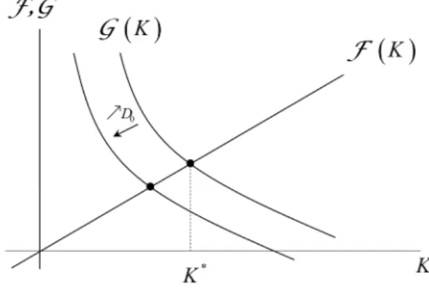
Introducing (A.5) and (A.4) in (A.3), we obtain an implicit relation in K F(K) =G(K),
where F(K) :=A[1−τ(1−α)]K, and G(K) :=A(1−τ)(1−α)/αρA011−−αε K−ε−αAD
0. Clearly, asGis a monotonic decreasing continuous function, according to the intermediate value theorem, there is a unique critical value K∗ >0 such that F(K∗) =G(K∗) for an
usual constellation of parameters. From Eqs. (A.4)-(A.5), we find the associated long-run values of C∗ and G∗.
In addition, as G(·) negatively depends onD0, any increase in public debt reduces the long-run capital stock (see Figure A.8).
Figure A.8: The steady state
It is straightforward to show that the steady-state is well determined, independently of the public debt level. Effectively, denoting X := eλ0+λ1˜k∗+λ2˜c∗, the determinant of
system (A.1)-(A.2) is, in the neighborhood of the steady state (˜c∗,k˜∗),
det =λ1αXec˜ ∗−˜k∗ +λ2αX[e˜c ∗−k˜∗ −D0Xe−˜k∗]<0, since, by (A.1), e˜c∗−˜k∗ −D0Xe−k˜∗ = [1−τ(1−α)]X >0.
Therefore, in a neoclassical (exogenous) growth model with public spending being the adjustment variable in the government’s budget constraint, a constant public debt D0 reduces the long-run capital stock K∗, without generating multiplicity of long-run solutions or indeterminacy of the transition path. This result generalizes GH’s findings to balanced-budget rules associated with a positive debt level.
Appendix B. Proof of Theorem 1
• Zero-growth solution. From the Keynes-Ramsey relation (11), we have: γ = ˙C/C = 0 ⇔ αyk = ρ. Consequently, the zero-growth solution (denoted by point Z in Figures 3-6) is characterized by cZ k = / ρ αA 01/ψ >0. From (18), γZ = 0 ⇔ ( ¯d+α+αdZ k)ykZ−cZk = 0. Thus, as cZk >0, we have dZk = 1 α " 1 A(cZ k)ψ−1 −d¯−α # .
The existence of the zero-growth solution (namely dZ
k > 0) is ensured if ρ < ρ¯:=
αA[A( ¯d+α)]ψ/(1−ψ).
• Non-zero growth solutions. As dk = 0, we have, using Eq. (17),
Ψ(ck) := ck−ρ−dAc¯ ψk = 0. (B.1) The behaviour of function Ψdepends on the sign of ψ.
(i) ψ < 0 ⇔ φ < 1 +ε. In this case, Ψ describes an increasing convex curve for ck ∈ (0,+∞), where Ψ(0) = −∞ and Ψ(+∞) = +∞. According to the Intermediate Value Theorem, there is a unique critical value cQk > 0 such that Ψ(cQk) = 0.
Besides, in the long run, the growth rate is γ =αAcψk −ρ; hence
γ ≥0⇔ 1 ck ≥cZk if ψ >1, ck ≤cZk if ψ <0. Consequently, if Ψ(cZ k) > 0, i.e. ρ < ρ¯, we have c Q
k < cZk, and the growth rate is positive at point Q= (cQk,0).
(ii) ψ > 0 ⇔φ >1 +ε. In this case, Ψ′(ck) ≥ 0⇔ c
k ≤ ˆck := (ψdA¯ )1/(1−ψ), with Ψ(0) =−ρ<0, and Ψ(+∞) =−∞, since ψ >0⇒ψ >1.
Thus, if Ψ(cZ
k) >0, namely ρ < ρ¯, according to the Intermediate Value Theorem, there are two positive solutions: cN
k < cZk, and cPk > cZk; hence, the economic growth rate is negative at point N = (cN
k,0) and positive at point P = (cPk,0). Appendix C. Proof of Theorem 2
We study the local stability of the steady states in the two regimes.
(i) Zero-growth solution. At point Z, as γZ = 0, we have, from Eq. (26), det(JZ) = −ψα2(yZ
k)2dZk.
• If ψ > 0 (regime R2), det(JZ) < 0, which means that there are two opposite-sign eigenvalues, and Z is a saddle-point.
• If ψ < 0 (regime R1), det(JZ) > 0, and, from Eq. (25), Tr(JZ) = cZ
k −ψdy¯kZ −
αdZ
kykZ[ψ+1] =yk[( ¯d+α)−( ¯d+αdZk)ψ]>0. Consequently, there are two eigenvalues with positive real part, and Z is unstable (over-determined).
(ii) Non-zero growth solution. As di
k = 0, from Eq. (26), det(Ji) = −[cki −d¯ψyki]γi, and Tr(Ji) =ci
• If ψ < 0 (regime R1), there is a unique non-zero growth solution (point Q). As
γQ >0, we have det(JQ)<0, namely, Q is a saddle-point.
• If ψ > 0 (regime R2), cik−d¯ψyik < 0 ⇔ cik > ˆck := [1/dA¯ ψ]1/(ψ−1). As cNk < ˆck, and γN < 0 (see Appendix B), we have det(JN) > 0, and Tr(JN) > 0, namely, N is unstable (over-determined). In contrast, as cP
k > ˆck and γP > 0, we have det(JP)>0, and Tr(JP)<0, namely,P is stable (under-determined).
Appendix D. Proof of Theorem 3
Let us define ζ(dk) := ¯d(dk) +αdk, with ¯d(dk) = (1−τ(dk))(1−α). As τ′(dk) ≥τˆ,
we have ζ′(dk) ≤ 0, ∀d
k ≥ 0. From system (27), as in section 3, there are two types of solutions: a zero-growth solution (dk > 0 ⇒ γ = 0), and non-zero growth solutions (γ >(<)0⇒dk= 0).
(i) Zero growth solution. Following the proof of Theorem 1, the zero-growth BGP (denoted by point Z in Figure 7) is still characterized by cZ
k = / ρ αA 01/ψ >0. Besides, we have γZ = 0⇔ cZk −ρ−ζ(dZk)A(cZk)ψ = 0⇔ζ(dZk) = c Z k −ρ A(cZ k)ψ .
As ζ is a continuous and monotonic function, there is an inverse function ζ−1, and dZk =ζ−1 2 cZ k −ρ A(cZ k)ψ 3 . As ζ :R+&→R+, this solution exists if:
(a) cZ k >ρ, i.e. ρ<ρˆ1 := (αA)1/(1−ψ), (b) (cZ k −ρ)/A(cZk)ψ <ζ(0), i.e. τ(0) <τ¯0 := 1− 1−1α - cZ k−ρ A(cZ k)ψ . .
(ii) Non-zero growth solutions. As dk = 0, for ck >0 we have, using Eq. (27) Φ(ck) :=ck−ρ−ζ(0)Acψk = 0,
hence,Φ′(ck)>0⇔ck<ˆck:= [Aψζ(0)]1/(1−ψ), with Φ(0) = −ρandΦ(+∞) = −∞<0. Consequently, if Φ(ˆck) > 0, i.e. ρ < ρˆ2 := ˆck(ψ −1)/ψ, according to the Intermediate Value Theorem, there are two positive solutions: ck<ˆck and ck >cˆk.
In addition, the condition (b) τ(0) < τ¯0 states that Φ(cZk) < 0, namely either cZk < ck < cˆk < ck or ck < cˆk < ck < cZk. Under the sufficient condition cZk < ˆck, i.e.
ρ<ρˆ3 :=αA[Aψζ(0)]ψ/(1−ψ), it is clear that cZk < ck< ck.
Therefore, there are three solutions: a zero growth solution (Z), and two positive growth solutions that we denote, respectively, the medium-growth solution (point M) corresponding to ck =: cM
k , and the high-growth solution (point H) corresponding to ck=:cHk.