Transition Induced by Tandem Rectangular Roughness
Elements on a Supersonic Flat Plate
Amanda Chou
∗, Rudolph A. King
†, and Michael A. Kegerise
‡ NASA Langley Research Center, Hampton, VA, 23681, USAThe flow behind two rectangular roughness elements with a height approximately 38– 41% of the boundary layer thickness was examined with a hot-wire probe. The rectangular roughness elements are oriented so that one element was at a +45-degree angle relative to the leading edge of the plate. A second roughness element was placed 7.16 mm down-stream of the first one with either the same orientation relative to the leading edge of the plate, or an opposing orientation of −45 degrees from the leading edge. Mean mass-flux and total-temperature profiles of the flow field downstream of the tandem roughness el-ements were examined for mean-flow distortion. Using streak strength as a measure of mean-flow distortion, the tandem roughness elements had approximately the same amount of distortion, regardless of their relative orientation. Mass-flux fluctuation profiles show that the dominant mode downstream of the tandem roughness elements with the same orientation was similar to that of a single roughness element and centered at a frequency of approximately 55 kHz. The dominant instability downstream of the tandem roughness elements with opposing orientation was centered at a frequency of 65 kHz and grew more slowly than the instabilities behind the single roughness element.
Nomenclature
AST streak amplitude
Aρu streak strength based on mass flux, kg/(m2-s) f frequency, Hz
k height of roughness element,µm
L length of roughness element, mm
M Mach number
p pressure
Pxx auto-spectra density r hot-wire recovery factor
Red wire Reynolds number, m-1 T temperature, K
u velocity, m/s
w width of roughness element, mm
x streamwise direction on flat plate, mm
x0 location of most downstream roughness
element, mm
y vertical direction on flat plate, mm
z spanwise direction on flat plate, mm
δ boundary layer thickness, mm
∂(ρu)
∂y wall-normal mass-flux shear, kg/(m
3-s)
∂(ρu)
∂z spanwise mass-flux shear, kg/(m
3-s)
η non-dimensional boundary layer parameter
µ dynamic viscosity, Pa-s
ρu mass flux, kg/m2·s
τ hot wire overheat ratio Subscript
∞ freestream condition 0 stagnation condition
0.995 condition whereu/u∞= 0.995 r recovery condition
w wire condition Superscript
0 fluctuating quantity
Abbreviations and Acronyms
CTA constant temperature anemometer RMS root-mean-square quantity
SLDT Supersonic Low Disturbance Tunnel ∗Research Aerospace Engineer, Flow Physics & Control Branch, M/S 170, AIAA Senior Member.
†Research Aerospace Engineer, Flow Physics & Control Branch, M/S 170, Member AIAA. ‡Research Scientist, Flow Physics & Control Branch, M/S 170, AIAA Senior Member.
I.
Introduction
The subject of roughness-induced transition in high-speed flows is of concern for practical geometries and vehicles. Manufactured surfaces have an inherent distributed roughness and fasteners or sensors can result in patterns of isolated roughnesses. These necessary real-life features can make an otherwise smooth surface rough. Given that roughness is unavoidable on practical vehicles, it is critical to determine its impact on boundary-layer transition. To that end, the physical mechanisms by which roughness causes transition must be better understood and incorporated into transition models. The onset of transition may be caused by a variety of factors including the enhancement of receptivity to the external disturbances,1 the transient
growth of boundary-layer perturbations, the acceleration of the growth of existing instability modes in the boundary layer,2and the wake instabilities induced by the roughness itself.3, 4
Much of the literature regarding high-speed boundary-layer transition concerns the sizing of roughness trips to induce transition. Knowing how to size an effective trip can help designers determine an acceptable limit for manufacturing tolerances. Large isolated roughnesses can cause transition through the production of a wake instability driven by an absolute instability upstream. Smaller isolated roughnesses can cause transition by amplifying a boundary-layer instability present upstream even when the integrated growth potential of the wake instability is not enough to incite transition.2 Discrete roughness elements are also
used to modulate the boundary layer in order to delay transition. Arrays of discrete roughness elements were used on swept wings to excite a stable wavelength of crossflow vortices.5–7 Studies of arrays of isolated
roughness elements can provide insight into the interaction of these elements.
Current methods of predicting transition location resulting from roughness include algebraic methods and semi-empirical methods. Algebraic methods empirically correlate some transition parameter with a disturbance parameter. Because the parameter space in which roughness can be defined is large, the algebraic correlations typically require tuning or biasing the correlations for each environment, geometry, and roughness type (isolated or distributed).8–10 Semi-empirical methods are currently being developed as well for wake
instabilities.2 However, to develop these methods, more information on which instabilities dominate in the wake of a roughness element is required.
Different types of instabilities can be found in the wake of small roughness elements. These wake insta-bilities are typically defined as an odd (sinuous) mode or an even (varicose) mode for a symmetric roughness element. The wake of a roughness element is typically characterized by an upwelling of fluid creating mushroom-like structures in the mean flow. These secondary flow structures are created by the shear forces in the fluid. The odd mode is found in regions where the spanwise shear is greater, typically on either side of the upwelling of fluid behind the roughness element. The even mode is found in the regions where the wall-normal shear is greater, typically centered at the top of the upwelling of fluid behind the roughness element.11 For asymmetric roughness elements, there are similar families of eigenmodes, but they are not
referred to as even or odd modes.
Some direct numerical simulations have been done for a single isolated roughness element on a flat plate at Mach 3.5.12 These simulations showed the effect of two-dimensional and three-dimensional disturbances
interacting with the roughness element. Symmetric isolated roughness elements such as a diamond planform can produce symmetric wakes when the freestream disturbances interacting with the roughness are considered to be two-dimensional. This produces the even and odd modes described in Ref. 11. When a planar wave at an angle interacts with the roughness element, the disturbance field in the wake of the roughness element skews along the same direction as the inclined plane wave. The mean flow supports both the odd and even eigenmodes and the inclined plane wave seeds both modes.12
Studies of these instability modes in the wake of isolated roughness elements have shown good agreement between experiments and computations.13 An experiment by Kegerise et al.14 showed the effect of a single
roughness element with different planforms on the growth of disturbances downstream. These roughness elements all had a consistent frontal area roughness height of approximately 48% of the boundary layer thickness for a nominal roughness Reynolds number of 462. Kegerise et al. were able to make detailed surveys downstream of the isolated roughness elements to determine the instability modes present in the wake. These were compared to linear stability theory, and for the case of the diamond planform roughness element, good agreement between the computations and experiments occurred close to the roughness element where linear growth occurred. However, once the wake instabilities became nonlinear, the linear stability theory no longer matched. The instability growth rates for the asymmetric planform appeared to be lower than those for the symmetric planform, so transition onset was delayed relative to the symmetric planform.14 The study of isolated roughness elements is important in determining the physical mechanisms that affect
transition in the wake of roughness elements. However, real vehicles can have multiple isolated roughness elements or distributed roughness. Thus, it is desirable to also study the effect of the interactions between these roughness elements to determine the physical mechanisms responsible for transition behind these types of roughness. Early work by Carmichael measured the transition Reynolds number on a flat plate due to the presence of arrays of roughness elements in a subsonic facility.15 Carmichael investigated the effect
of grids of cylindrical roughness elements, streamwise rows of roughness, and spanwise rows of roughness. Carmichael also varied the heights and diameters of the roughness elements in the different configurations. For the streamwise arrays of roughness, Carmichael found that there was less of an effect, and likely, less interaction between roughness elements spaced more than three diameters apart. Noting that the parameter space to study was large, Carmichael examined only the transition location for these patterns of roughness elements.
Choudhari et al. looked at the effect of two tandem roughness trips with diamond-shaped planforms.11
The computations examined the effect of height on the amplitude of the streaks downstream of the roughness trips induced by the wake instability. The addition of a downstream isolated roughness had an effect on the streak amplitude when the roughness was short (k/δ0.995 = 0.15) and less of an effect on the streak
amplitude when the roughness was taller (k/δ0.995= 0.37). Choudhari et al. proposed that this is due to the
ability of the flow field to recover after the first roughness trip and the receptivity of the second roughness trip to the wake behind the first roughness trip.
The effect of tandem circular roughness elements was investigated in Ref. 16. Two different roughness heights and four different configurations of roughness elements were tested for each roughness height. The roughness elements were nominally 140 µm and 280 µm in height, resulting in a k/δ of 0.17–0.41 at the station of the most downstream roughness element. Little to no growth occurred in the wake instabilities behind the shorter roughness elements. The shorter roughness elements also showed the presence of a very weak odd-mode instability centered near 35 kHz at the most downstream measurement station. The wake instabilities behind the tallest roughness elements grew and experienced breakdown in the measurement region. The wake broke down at the same distance behind the most downstream of the tandem roughness elements that were spaced 2D apart from center to center, regardless of the number of roughness elements in the streamwise array. At a spacing of 4Dapart from center to center, transition moved upstream relative to the most downstream of the roughness elements in the streamwise array. The wake instability behind the tallest roughness element appeared to be an even mode centered around 80 kHz.
In this paper, wake instabilities behind tandem rectangular roughness elements oriented at a 45-degree angle relative to the leading edge of a flat plate were measured to investigate the effect of asymmetric roughness elements. The mean mass flux, total temperature, and fluctuating mass flux were measured behind these arrays of roughness elements and used to determine the type of instabilities present in the wake of these roughness elements. The mean flow properties were used to show the mean flow distortion and the relative shear in the mass flux behind the roughness elements. The fluctuating mass flux was used to identify instabilities present in the wake of these roughness elements and to determine the growth of these instabilities.
II.
Facility and Equipment
A. Supersonic Low Disturbance Tunnel
These experiments were conducted in the NASA Langley Research Center Supersonic Low Disturbance Tunnel (SLDT), a Mach-3.5 quiet facility.17 A two-dimensional nozzle with exit dimensions of 15.24 cm by 25.40 cm (6 in. by 10 in.) was used in the SLDT. The stagnation pressure for this experiment was 206.8±2.6 kPa and the stagnation temperature was 319.3±2.1 K. The performance of the nozzle was similar to the performance measured by Kegerise et al.14 At these conditions, the freestream mass-flux fluctuations stayed well below 0.05% on the centerline until a location approximately 360 mm from the nozzle throat.
B. Flat Plate Model
The flat plate model was positioned so that the nominally-sharp leading edge of the plate was 140 mm from the nozzle throat, well within the uniform flow region. The flat plate was 228.6 mm wide at the leading edge and 406.4 mm long. Most of the measurements on the flat plate model were taken within the quiet core of
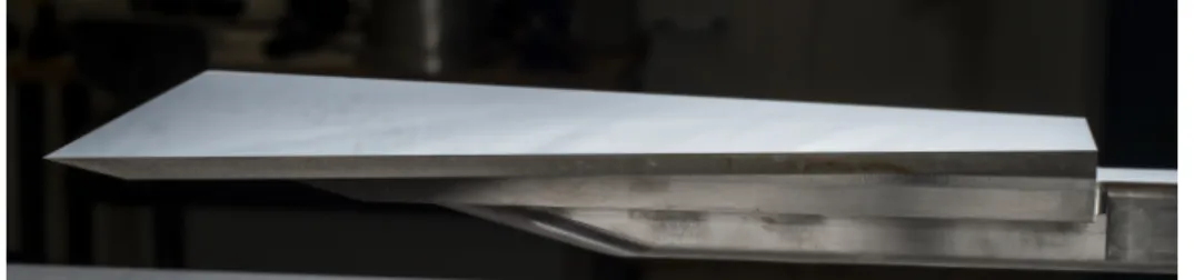
the facility, so the measurement region ends approximately 220 mm from the leading edge of the plate. This helps to reduce ambiguity regarding the effects of the freestream disturbance level. The upper surface of the plate, where measurements were made, was polished to a mirror finish (0.025-µm RMS roughness) and the sides of the flat plate were tapered to reduce edge effects. The trailing edge of the flat plate was 76.2 mm wide. A picture of the flat plate model is provided in Fig. 1.
Figure 1. A side view of the polished flat plate. Measurement surface is toward the top of the picture.
C. Roughness Elements
Measurements were made behind rectangular roughness elements oriented 45°from the leading edge of the flat plate (Fig. 2). These rectangular roughness elements were nominally 3.58-mm long, 1.19-mm wide, and 280-µm tall. The height of each of the roughness elements was then measured with a stylus-based surface profilometer. Variation in the roughness height for each of these roughness elements was no more than±2.5% of the nominal height. These roughness elements were positioned so that the farthest upstream roughness element was centered at a location of 41.5 mm from the leading edge of the flat plate, where k/δ ≈0.41. Three configurations of the roughness element were tested: a single rectangular roughness element rotated to be +45°from the leading edge, two rectangular roughness elements (tandem roughness elements) oriented +45° from the leading edge, and two rectangular roughness elements (tandem roughness elements) with one oriented at +45° from the leading edge and the other oriented −45° from the leading edge. These configurations are illustrated in a schematic in Fig. 3. A template was used to align the roughness elements on the flat plate so that the downstream roughness element was aligned relative to the first roughness element. The template also fixes or sets the streamwise location of each roughness element. Each roughness element was affixed with a cyanoacrylate glue to the surface of the polished flat plate. The distances between each roughness element were fixed by the template at a center-to-center spacing of two lengths (2L) apart so that
k/δ= 0.38 for the second roughness element.
k
L w
Figure 2. A schematic of the roughness elements used: L= 3.58mm,w= 1.19mm,k≈280µm.
D. Hot-Wire Measurements
Hot-wire anemometry was used to probe the boundary layer in the wake of the roughness elements, following the approach documented by Kegerise et al.18 The sensing element for the boundary-layer probes was a 3.8-µm platinum-plated tungsten wire with a nominal length of 0.5 mm. The hot wires were tuned to have a bandwidth of approximately 370 kHz. The hot wire was operated at a high overheat ratio in order to be more sensitive to mass flux. The cold wire resistance was also measured at each measurement station to correct for the total temperature change in the boundary layer.18 The measurements were passed through
a signal conditioner that had a low-pass filter cutoff at 400 kHz and a high-pass filter cutoff at 1k Hz. The signal was sampled at 1 MHz for one second at each measurement location.
x0 +x
M
∞+z
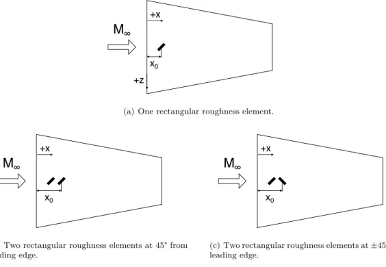
(a) One rectangular roughness element.
x0 +x
M
∞(b) Two rectangular roughness elements at 45°from leading edge.
x0 +x
M
∞(c) Two rectangular roughness elements at±45°from leading edge.
Figure 3. A schematic of the different configurations of roughness elements tested.
III.
Results
A. Mean Profiles of Mass Flux and Total Temperature
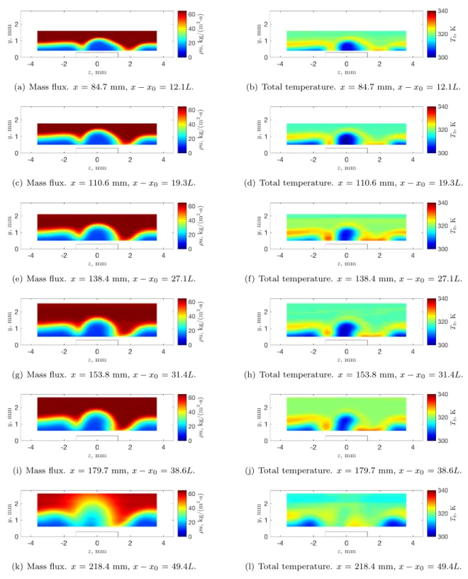
Measurements of the mean mass flux and total temperature are presented as contour plots in Figs. 4–6. Since the freestream conditions remained constant throughout the experiment, these values are presented as dimensional values and the scaling for each of the contour plots remains the same. The mean mass flux and mean total temperature are plotted in Fig. 4, where the mean mass flux at each streamwise station where data were acquired is presented in the left column and the mean total temperature at each streamwise station is presented in the right column. The mean mass flux and mean total temperature contours qualitatively show the amount of mean flow distortion present in the boundary layer downstream of the roughness elements. The total temperature profiles are not shown for the other configurations for brevity. A quantitative measurement of the amount of distortion is given by the streak strength, presented in the next section.
Unlike the symmetric wake behind a circular roughness element,16, 18 the wake behind the angled
rect-angular roughness element is asymmetric, as expected. The wake of the single roughness element near the centerline (Fig. 4) shows a large, asymmetric upwelling of fluid near the centerline of the wake. The upwelling of flow near the center of the wake of the roughness elements is biased toward the−z-direction for the first two measurement stations (Figs. 4(a) and 4(c)). At farther downstream stations, this upwelling of flow near the center begins to bias toward the +z-direction (Figs. 4(e)–4(l)).
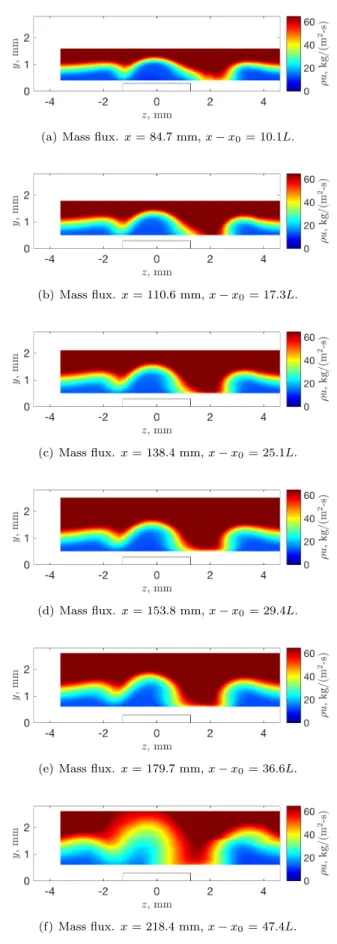
Like the single roughness element, there is also an upwelling of fluid along the centerline of the wake behind the tandem roughness elements with the same orientation. For the tandem roughness elements with the same orientation (both +45°from the leading edge), the centerline upwelling of fluid appears to be biased toward the−z-direction at only the first measurement station (Fig. 5(a)). The tandem roughness elements with the same orientation also show a slightly thicker boundary layer between z = 2 and 3 mm. There is also a larger deficit of fluid betweenz= 1 mm and 2.5 mm, which may indicate a slightly stronger vortical structure in the wake of the tandem roughness elements.
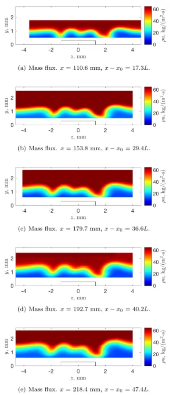
The tandem roughness elements with opposite orientation (one at +45 and one at−45°from the leading edge) appear to have less distortion and more uniformity across the span (Fig. 6)). Unlike the single roughness element, the wake near the centerline does not show the same upwelling of fluid behind the tandem roughness elements with opposite orientation. Toward the +z-direction, the boundary layer thickness also appears to
(a) Mass flux. x= 84.7 mm,x−x0= 12.1L. (b) Total temperature. x= 84.7 mm,x−x0 = 12.1L.
(c) Mass flux. x= 110.6 mm,x−x0 = 19.3L. (d) Total temperature. x= 110.6 mm,x−x0 = 19.3L.
(e) Mass flux. x= 138.4 mm,x−x0 = 27.1L. (f) Total temperature. x= 138.4 mm,x−x0 = 27.1L.
(g) Mass flux.x= 153.8 mm,x−x0= 31.4L. (h) Total temperature. x= 153.8 mm,x−x0 = 31.4L.
(i) Mass flux. x= 179.7 mm,x−x0 = 38.6L. (j) Total temperature.x= 179.7 mm,x−x0= 38.6L.
(k) Mass flux. x= 218.4 mm,x−x0= 49.4L. (l) Total temperature.x= 218.4 mm,x−x0= 49.4L. Figure 4. Mean measurements behind a single rectangular roughness element oriented 45-degrees from the leading edge of the flat plate (k≈280µm).
thicken near the edges of where the roughness element lies, betweenz= 2 and 3 mm. This thickening was also observed for the tandem roughness elements with the same orientation, so it is possible that the addition of a downstream roughness element in either direction diverts some extra fluid in the wake toward the outer edges.
(a) Mass flux.x= 84.7 mm,x−x0= 10.1L.
(b) Mass flux. x= 110.6 mm,x−x0 = 17.3L.
(c) Mass flux. x= 138.4 mm,x−x0 = 25.1L.
(d) Mass flux. x= 153.8 mm,x−x0 = 29.4L.
(e) Mass flux. x= 179.7 mm,x−x0 = 36.6L.
(f) Mass flux. x= 218.4 mm,x−x0= 47.4L.
Figure 5. Mean measurements behind two rectangular roughness elements, both oriented 45-degrees from the leading edge of the flat plate (k≈280µm).
(a) Mass flux.x= 110.6 mm,x−x0= 17.3L.
(b) Mass flux. x= 153.8 mm,x−x0 = 29.4L.
(c) Mass flux. x= 179.7 mm,x−x0 = 36.6L.
(d) Mass flux. x= 192.7 mm,x−x0 = 40.2L.
(e) Mass flux. x= 218.4 mm,x−x0 = 47.4L.
Figure 6. Mean measurements behind two rectangular roughness elements, with opposing orientation ±45 -degrees from the leading edge of the flat plate (k≈280µm).
B. Streak Strength
The mean-flow distortion in the wake of roughness elements can be quantified by the relative amplitude of the high-speed and low-speed regions behind the roughness. The streak amplitude is defined by Fransson et al. as the wall-normal maximum of the peak-to-peak difference between the streamwise velocities:
AST =
1 2max
n
where U(y)high and U(y)low are the velocity profiles in a high-speed and low-speed streak region,
respec-tively.19 The streak strength in this paper is based on ρubecause the hot-wire measurements are sensitive to mass flux in compressible flow. For these data, a streak strength is defined as
Aρu=
1 2
ρu(y)high−ρu(y)low (2)
and the streak amplitude is defined as the wall-normal maximum of the streak strength profile. These streak strength profiles are nondimensionalized by the edge mass flux of the profiles and the height in the boundary layer is given by the nondimensional boundary layer parameter
η=y
r
Re
x (3)
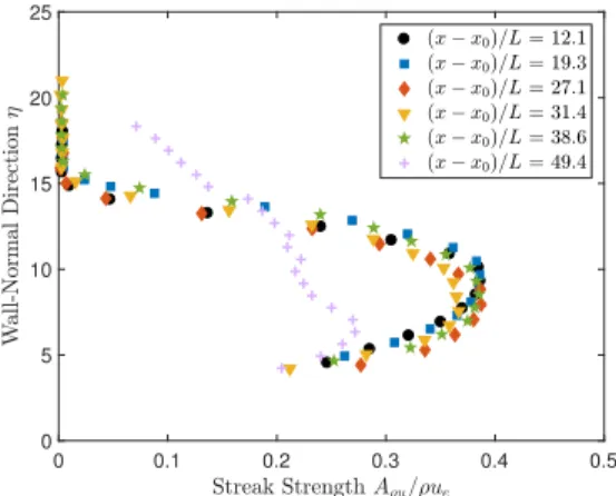
wherey is the height above the surface of the flat plate andRe is the freestream unit Reynolds number. The streak strength profiles for the different roughness configurations are shown in Fig. 7. The maximum in streak strength stays relatively constant as measurements are taken farther downstream of the array of roughness elements, except at the last measurement station. As with the contour plots of mean mass flux and total temperature, the streak strength profiles appear similar for the first two configurations of rectangular roughness elements: the single roughness element at +45°and the tandem roughness elements with the same orientation. This is similar to the effect seen behind circular roughness elements with a spacing of 2Dapart.16 The streak strength profile at the farthest downstream measurement station behind the single roughness element becomes flatter, presumably due to the breakdown of the flow to turbulence. The streak strength profile at the farthest downstream measurement station behind the tandem roughness elements decreases in amplitude, but does not flatten out as it did in the wake of the single roughness element. This measurement is taken farther upstream relative to the most downstream roughness element, so it is possible that the flow is not as far along in the breakdown process at the last measurement station for this configuration. The suspected breakdown will be shown in the power spectra and the RMS mass-flux fluctuation profiles.
Using this standard of quantifying the mean flow distortion, the distortion behind the tandem roughness elements with opposite orientation is only marginally less than the other configurations. The only major difference between the streak strength profile for this roughness configuration to the previous ones is that the streak strength profile at the most downstreamx−x0station remains at approximately the same magnitude
as the upstream stations. The peak in the streak strength profiles in Fig. 7(c) also appears slightly narrower than the streak strength profiles in Figs. 7(a) and 7(b).
The streak amplitude is simply a method of quantifying the amount of mean flow distortion. Thus, that the amplitudes for the streak strength are fairly similar for the three different configurations reveals little about the underlying physical mechanisms that induce transition. In that case, looking at the fluctuating quantities and frequency content of the fluctuations is necessary.
C. Power Spectra
Power spectra were computed using the Welch spectrum estimation method, applying Hanning windows to 2048-point windows, 50% overlap of the windows, and then averaging the samples over the one-second data acquisition period. This yields a frequency resolution of 488 Hz. The spectra selected for each x−x0
station corresponds to the point in the survey plane at which the RMS amplitude was largest. The location where the highest RMS amplitude was found was limited to a region fromz=−1.5 toz = 0.5 mm for the single roughness element and the tandem roughness elements with the same orientation and from z =−2 to z = 2 mm for the tandem roughness elements with opposite orientation. This was to ensure that the same instability was being tracked at each downstream station and the reasoning behind the selection of the regions will be illustrated in the next section. A comparison of the power spectra at each streamwise station is provided in Fig. 8.
Several different peak frequencies appear in the power spectra of the measurements made downstream of the single roughness element (Fig. 8(a)). The suspected instabilities had peak frequencies centered at 55 kHz, 75 kHz, and 95 kHz. At a location ofx−x0= 31.4Lfrom the single roughness element, the peaks at
around 55 kHz and 95 kHz appear to be the same amplitude and the 75-kHz peak is no longer distinguishable as a separate peak. Atx−x0 = 38.6L, the 95-kHz instability starts to increase slightly in frequency, and
0 0.1 0.2 0.3 0.4 0.5 0 5 10 15 20 25
(a) 1 rectangular roughness atx0= 41.5 mm.
0 0.1 0.2 0.3 0.4 0.5 0 5 10 15 20 25 (b) 2 rectangular roughnesses, at 45°. 0 0.1 0.2 0.3 0.4 0.5 0 5 10 15 20 25 (c) 2 rectangular roughnesses, at±45°.
Figure 7. Streak strength profiles for rectangular roughness elements in a streamwise array (k≈280µm).
the harmonic to the kHz instability appears in the spectra. At farther downstream stations, the 55-kHz instability appears to dominate the spectral content and grows until the last measurement station. At
x−x0= 49.4L, the spectrum broadens significantly, but the 55-kHz instability is still of higher amplitude
than atx−x0= 38.6L. This indicates that the flow is starting to break down at the last station.
Downstream of the tandem roughness elements with the same orientation, similar instability peaks as for the single roughness element are present in the spectra (Fig. 8(b)). The dominant instability peak appears to be at 75 kHz atx−x0= 17.3L, but is quickly dominated by the 55-kHz instability at all other downstream
stations. The first harmonic of the 55-kHz instability also becomes more evident in the spectra at the location of x−x0= 39.0L. At the farthest downstream station ofx−x0 = 47.4L, the spectrum broadens but the
55-kHz instability has still grown compared to its amplitude atx−x0= 39.0L. As with the single roughness
element, the flow is likely starting to break down.
The final dominant instability in the measurements downstream of the tandem roughness elements with opposite orientation appears to be of a different frequency than the previous two roughness configurations (Fig. 8(c)). At the farthest upstream station ofx−x0 = 17.3L, the peak instability lies at approximately
55 kHz. Slightly downstream, at x−x0 = 29.4L and 33.0L, a 55-kHz peak and a 75-kHz peak appear
in the spectra as for the other two roughness configurations. A small peak at 95 kHz also appears in the spectra at these streamwise locations, and grows slightly before disappearing. The amplitude of this 95-kHz peak is approximately one order of magnitude less than the other instabilities. At x−x0 = 36.6L and
farther downstream, one broad instability peak centered at 65 kHz appears in the spectra. This instability peak grows with downstream distance, but the spectra do not show evidence of broadening at the farthest downstream measurement stations, nor the presence of harmonics for this peak at the downstream stations. The wake of the tandem roughness elements with opposite orientation likely does not break down nor become
103 104 105 106 10-14 10-12 10-10 10-8 10-6 10-4 10-2
(a) 1 rectangular roughness element atx0= 41.5 mm.
103 104 105 106 10-14 10-12 10-10 10-8 10-6 10-4 10-2
(b) 2 rectangular roughness element, at 45°.
103 104 105 106 10-14 10-12 10-10 10-8 10-6 10-4 10-2
(c) 2 rectangular roughness element, at±45°.
Figure 8. Power spectra taken at the location with the largest RMS for the most-amplified disturbance in a planar survey.
nonlinear in the available measurement region.
D. RMS Mass Flux Fluctuations
The RMS mass-flux fluctuations within a 5-kHz bandwidth for several frequencies were computed for each measurement location behind the roughness elements. The RMS mass-flux fluctuations are normalized by the edge mass flux. The contour plots are divided so that the columns of each figure correspond to different instability frequencies and the rows of each figure correspond to a different x−x0 location. The contour
levels for each of the plots is the same across the rows so that the amplitude of the instabilities at eachx−x0
station are presented on the same scale. The contour levels change between thex−x0stations so that the
mode shapes can be more easily identified.
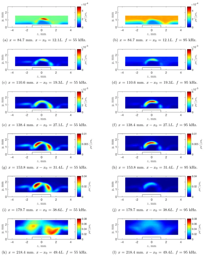
The peak frequencies in Figs. 8(a) occur at approximately 55, 75, and 95 kHz. At x−x0 = 31.4L,
the 75-kHz instability is no longer one of the dominant disturbances in the power spectra and the 95-kHz instability grows larger. Thus, the data for the 75-kHz instability are not shown in the contour plots in Fig. 9. In the end, the 55-kHz instability appears to dominate and persist until the last measurement station at
x−x0= 49.4L. The progression of the 55-kHz instability at each streamwise station is shown for the single
roughness element in the left column of Fig. 9. At the upstream locations ofx−x0= 12.1Land 19.3L, the
55-kHz instability appears to be centered at a location approximately 0.2 mm toward the +z-direction with smaller regions of increased fluctuations to either side. Atx−x0= 27.1L, the higher-amplitude fluctuations
appear to be centered closer to z =−0.6 mm. The 55-kHz instability is visibly distributed on either side of the centerline of the wake of the single rectangular roughness element at x−x0 = 31.4L and farther
downstream (Figs. 9(g)–9(k)). Higher amplitude fluctuations in the 55-kHz band appear to be concentrated toward the−z-direction. This mode grows and eventually starts to break down afterx−x0= 49.4L, which
is the farthest downstream that measurements were made on the flat plate.
(a)x= 84.7 mm. x−x0 = 12.1L.f = 55 kHz. (b)x= 84.7 mm. x−x0= 12.1L. f= 95 kHz. (c)x= 110.6 mm.x−x0 = 19.3L.f = 55 kHz. (d)x= 110.6 mm. x−x0= 19.3L.f= 95 kHz. (e)x= 138.4 mm.x−x0 = 27.1L.f = 55 kHz. (f)x= 138.4 mm. x−x0= 27.1L. f= 95 kHz. (g)x= 153.8 mm. x−x0= 31.4L.f = 55 kHz. (h)x= 153.8 mm. x−x0= 31.4L.f= 95 kHz. (i)x= 179.7 mm.x−x0 = 38.6L.f = 55 kHz. (j)x= 179.7 mm.x−x0 = 38.6L.f = 95 kHz. (k)x= 218.4 mm. x−x0= 49.4L. f= 55 kHz. (l)x= 218.4 mm.x−x0= 49.4L.f = 95 kHz. Figure 9. RMS mass-flux fluctuations atf = 55 kHz (left column) andf= 95kHz (right column) behind one rectangular roughness element, oriented 45-degrees from the leading edge of the flat plate.
The change in the location of this region of higher-amplitude fluctuations may be related to the change in the mean flow. It may also be due to the presence of several different eigenmodes growing at different rates. Each mode occurs over a range of frequencies that overlap, so one mode may dominate and grow
faster initially before another one grows larger farther downstream. Unfortunately, the modes cannot be distinguished from each other as these measurements are made with a single-point measurement technique. The progression of the 95-kHz instability at each streamwise station is shown for the single roughness element in the right column of Fig. 9. The 95-kHz instability in the wake of the single roughness element appears to be concentrated near the centerline of the wake at the upstream stations ofx−x0= 12.1Land
19.3L(Figs. 9(b) and 9(d)). At stations ofx−x0= 27.1Land farther downstream, the higher-amplitude
fluctuations in the 95-kHz instability band begins to skew toward the−z-direction (Figs. 9(f)–9(l)). However, the region of the highest-amplitude fluctuations at 95 kHz remains closer to the centerline than the 55-kHz peak. As discussed previously, this is probably linked to the changes in the shape of the mean flow at these stations. Unlike the 55-kHz instability, the 95-kHz instability remains mostly concentrated in a single region even at the last measurement station ofx−x0= 49.4L.
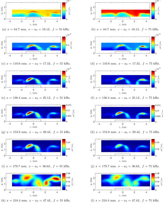
In the wake of the tandem roughness elements with the same +45°orientation to the leading edge, the dominant instabilities identified in the power spectra appear to be centered at 55 kHz and 75 kHz (Fig. 8(b)). Like the 55-kHz instability behind the single roughness element, the 55-kHz instability behind the tandem roughness elements is still the most dominant mode up to the last measurement station ofx−x0= 47.4L.
The addition of a roughness element did not change the dominant wake instability for a symmetric roughness element,16 so that this also holds true for an asymmetric roughness element is consistent. That the
closely-spaced asymmetric roughness elements with the same orientation behave like the closely-closely-spaced circular roughness elements in Ref. 16 suggests that the interaction between closely-spaced elements does not change the overall physical mechanisms that cause transition.
The RMS fluctuations of the mass flux in a 5-kHz band around these two frequencies is shown in Fig. 10. The left column corresponds to the RMS fluctuations atf = 55 kHz and the right column corresponds to the RMS fluctuations atf = 75 kHz. The 55-kHz instability in the wake of the tandem roughness elements with the same orientation are similar in shape to the same instability behind the single roughness element, except for some additional disturbances atz >2 mm. At the upstream station ofx−x0 = 10.1L, the instability
appears to be centered on the wake centerline (Fig. 10(a)). At stations of x−x0 = 17.3L and farther
downstream, the 55-kHz instability appears to be located on either side of the wake centerline (Figs. 10(c), 10(e), 10(g), 10(i), and 10(k)).
The 75-kHz instability in the wake of the tandem roughness elements with the same orientation appears similar to the 55-kHz instability. The RMS fluctuations at the farthest upstream measurement station of
x−x0 = 10.1L show the noise floor of the measurements (Fig. 10(b)). At x−x0 = 17.3L, Figs. 10(c)
and 10(d) appear to be similar, except that the region where higher-amplitude fluctuations occur seems to be centered closer to z = −1 mm for the 55-kHz instability and closer to z = −0.25 mm for the 75-kHz instability. Between x−x0 = 25.1L and 47.4L, the contour plots of the RMS mass flux fluctuation match
those of the 55-kHz instability fairly closely, except in amplitude (Figs. 10(e)–10(l)).
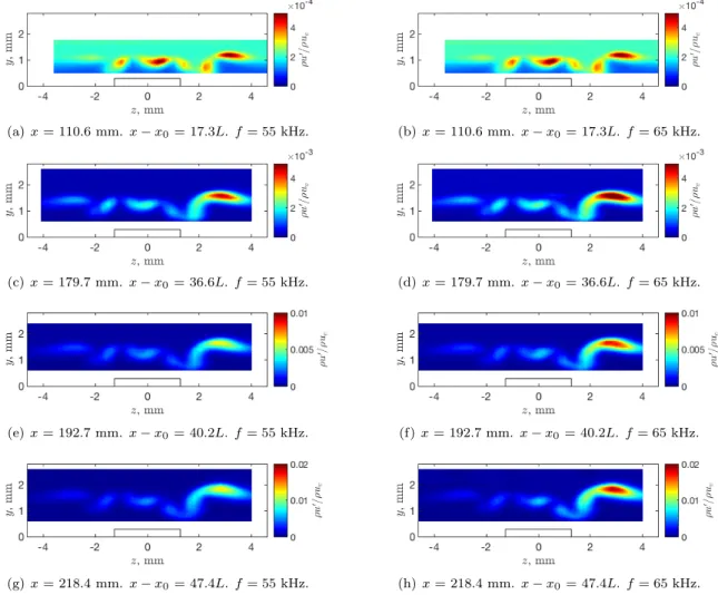
The dominant instability in the wake of the roughness elements with opposite orientation appears to be centered at 65 kHz (Fig. 8(c)). At the upstream stations ofx−x0= 10.1Lto 33L, the 55-kHz and 75-kHz
peaks appear in the spectra, but these quickly disappear and a broad peak centered at 65 kHz appears to dominate the spectra. For comparison, both the RMS fluctuations for 55 kHz and 65 kHz will be given in Fig. 11. The contours of the RMS fluctuations given in Fig. 11 show that the instabilities in the wake of the tandem roughness elements with opposite orientation remains consistent at several x−x0 stations.
Little change is seen in the shape of these contours, but the amplitude increases as the streamwise station increases. The distribution of the RMS fluctuations centered at 55 kHz and 65 kHz appear similar, so it is possible that these are essentially the same mode. The 65-kHz disturbance is fairly broad, so it may be that the appearance of the peak being centered at 65 kHz is a result of both a 55-kHz instability and a 75-kHz instability growing large and appearing to merge.
The dominant instability in the wake of the tandem roughness elements with opposite orientation appears to be a different mode shape than the other two configurations. This change is due to the change in the mean flow, which also alters which eigenmodes are supported by the mean flow. The amplitude of the mass-flux fluctuations in the third configuration is also more than an order of magnitude less than the amplitude of the fluctuations in the first two configurations. As expected, the power spectra and mode shape of this instability suggest that slower growth and a delay in transition occurs in the wake of the tandem roughness elements with opposite orientation. A higher-amplitude region centered around z = 3 mm is seen in the contour plots in Fig. 11. The RMS amplitude of the fluctuations in this region appears to grow larger than the fluctuations along the center of the wake. So, in tracking the growth of the wake instabilities, only the
(a)x= 84.7 mm. x−x0 = 10.1L.f = 55 kHz. (b)x= 84.7 mm. x−x0= 10.1L. f= 75 kHz. (c)x= 110.6 mm.x−x0 = 17.3L.f = 55 kHz. (d)x= 110.6 mm. x−x0= 17.3L.f= 75 kHz. (e)x= 138.4 mm.x−x0 = 25.1L.f = 55 kHz. (f)x= 138.4 mm. x−x0= 25.1L. f= 75 kHz. (g)x= 153.8 mm. x−x0= 29.4L.f = 55 kHz. (h)x= 153.8 mm. x−x0= 29.4L.f= 75 kHz. (i)x= 179.7 mm.x−x0 = 36.6L.f = 55 kHz. (j)x= 179.7 mm.x−x0 = 36.6L.f = 75 kHz. (k)x= 218.4 mm. x−x0= 47.4L. f= 55 kHz. (l)x= 218.4 mm.x−x0= 47.4L.f = 75 kHz. Figure 10. RMS mass-flux fluctuations atf = 55 kHz (left column) andf= 75kHz (right column) behind two rectangular roughness elements, with the same orientation 45-degrees from the leading edge of the flat plate.
disturbances in the centerline region are examined.
Because these roughness elements are not symmetric, their wake is not expected to be symmetric either. Thus, the identification of modes as being either odd or even may be misleading without the support of computational models. However, it may still be beneficial to determine how the spanwise and wall-normal shear correspond to regions of larger-amplitude fluctuations in the boundary layer. Since hot-wire measurements are sensitive to mass flux and not velocity, the spanwise derivative of the streamwise mass
(a)x= 110.6 mm.x−x0 = 17.3L.f= 55 kHz. (b)x= 110.6 mm. x−x0 = 17.3L.f= 65 kHz.
(c)x= 179.7 mm. x−x0= 36.6L.f= 55 kHz. (d)x= 179.7 mm. x−x0 = 36.6L.f= 65 kHz.
(e)x= 192.7 mm. x−x0= 40.2L.f= 55 kHz. (f)x= 192.7 mm. x−x0 = 40.2L.f= 65 kHz.
(g)x= 218.4 mm.x−x0 = 47.4L.f= 55 kHz. (h)x= 218.4 mm. x−x0 = 47.4L.f= 65 kHz. Figure 11. RMS mass-flux fluctuations behind two rectangular roughness elements, with opposite orientation
±45-degrees from the leading edge of the flat plate.
flux (∂(ρu)/∂z) is used to represent the spanwise shear of the mass flux. Likewise, the wall-normal shear of the mass flux is represented by the wall-normal derivative of the streamwise mass flux (∂(ρu)/∂y). There may appear to be some modulation in the wall-normal direction for these data, but this is due to the manner in which the data were acquired, not a physical phenomenon in the flow. The hot-wire data are acquired by traversing the probe in the spanwise direction and then increasing height. This means that the time at which data are acquired between the wall-normal points is much longer than the time at which data are acquired in the spanwise direction so small variations in the freestream appear large. In the following figures, the spanwise mass-flux shear and the wall-normal mass-flux shear are shown as color contours and the contours of the RMS fluctuations for different instabilities are shown as black lines.
For the single roughness element, the location of these instabilities relative to the wall-normal shear and spanwise shear are given in Fig. 12 for x−x0 = 19.3L and Fig. 13 for x−x0 = 31.4L. The rows
of these figures are for each of the dominant frequencies in the spectra. The left column of these figures corresponds to the spanwise mass-flux shear and the right column of these figures corresponds to the wall-normal mass-flux shear. At a location farther upstream, the 55-kHz, 75-kHz, and 95-kHz instabilities all appear to have a similar shape. The spanwise and wall-normal shear are both large at x−x0 = 19.3L.
The dominant instability at this station is centered at 75 kHz, which appears to have a higher magnitude in the same location where the wall-normal shear is large. The location where this instability has higher amplitude fluctuations corresponds to a location where there is almost no spanwise shear. The 55-kHz and 95-kHz instabilities also appear to be concentrated in areas where the shear in the wall-normal direction is greater. However, the 55-kHz instability is also concentrated in regions where the spanwise shear is high, nearz=−1 mm.
(a)f = 55 kHz (lines),∂(ρu)/∂z(color). (b)f = 55 kHz (lines),∂(ρu)/∂y(color).
(c)f= 75 kHz (lines),∂(ρu)/∂z(color). (d)f = 75 kHz (lines),∂(ρu)/∂y(color).
(e)f= 95 kHz (lines),∂(ρu)/∂z(color). (f)f = 95 kHz (lines),∂(ρu)/∂y(color).
Figure 12. A comparison of where boundary layer instabilities are concentrated relative to locations of spanwise and wall-normal shear for a single roughness element,x−x0= 19.3L.
At a farther downstream station of x−x0 = 31.4L, the 75-kHz disturbance is not very prominent in
the power spectra (Fig. 8(a)), so only the 55-kHz and 95-kHz instabilities are examined in Fig. 13. At this station, the 55-kHz instability and the 95-kHz instability take on two different shapes. The 55-kHz instability appears to be concentrated in the same location as where there is increased wall-normal mass-flux shear. At
x−x0= 19.3L, this mode appeared to be concentrated on the centerline, where the wall-normal mass-flux
shear was large. At x−x0 = 31.4L, the 55-kHz mode has higher amplitude fluctuations concentrated on
either side of the centerline of the wake, where the spanwise mass-flux shear is higher. The 95-kHz instability appears to be concentrated in the same location as where there is increased wall-normal mass-flux shear, and little change is seen betweenx−x0= 19.3Landx−x0= 31.4L.
For the tandem roughness elements with the same orientation, only the 55-kHz and 75-kHz instabilities are examined in Figs. 14 and 15 because the 95-kHz instability is not a peak in the power spectra for this configuration (Fig. 8(b)). Fig. 14 shows the location of the 55-kHz and 75-kHz instability relative to the spanwise and wall-normal shear at x−x0 = 17.3L. As in the case with a single roughness element, the
instabilities at a station close to the roughness element appear to lie in areas where the magnitude of both the spanwise and the wall-normal shear of the mass flux are large. The 55-kHz instability appears to span across the wake of the roughness element, where the region of higher-amplitude mass-flux fluctuations agree with regions of both increased spanwise and wall-normal mass-flux shear (Figs. 14(a) and 14(b)).
The 75-kHz instability also has higher-amplitude mass-flux fluctuations concentrated in the−z-direction at this station. This is the same region where the mass-flux shear in both the spanwise and wall-normal directions are large and approximately the same amplitude (Figs. 14(c) and 14(d)). The spanwise shear is approximately the same amplitude to either side of the centerline of the wake in Fig. 14(c), but of opposite sign.
At a slightly farther downstream station ofx−x0= 29.4L, the RMS contour plots of the instabilities at
55 kHz and 75 kHz appeared to be similar in shape (Figs. 10(g) and 10(h)). Fig. 15 shows the location of the 55-kHz and 75-kHz instability relative to the spanwise and wall-normal shear. At this station, both of
(a)f = 55 kHz (lines),∂(ρu)/∂z(color). (b)f = 55 kHz (lines),∂(ρu)/∂y(color).
(c)f= 95 kHz (lines),∂(ρu)/∂z(color). (d)f = 95 kHz (lines),∂(ρu)/∂y(color).
Figure 13. A comparison of where boundary layer instabilities are concentrated relative to locations of spanwise and wall-normal shear for a single roughness element,x−x0= 31.4L.
(a)f = 55 kHz (lines),∂(ρu)/∂z(color). (b)f = 55 kHz (lines),∂(ρu)/∂y(color).
(c)f= 75 kHz (lines),∂(ρu)/∂z(color). (d)f = 75 kHz (lines),∂(ρu)/∂y(color).
Figure 14. A comparison of where boundary layer instabilities are concentrated relative to locations of spanwise and wall-normal shear for tandem roughness element with the same orientation,x−x0= 17.3Lmm.
the instabilities now have higher amplitudes in regions corresponding to where the spanwise shear is large. The wall-normal mass-flux shear still has a fairly large magnitude, but it is difficult to say whether the wall-normal shear has as much of an effect on the generation of the instabilities here as atx−x0= 17.3L.
For the tandem roughness elements with opposite orientation, the contours of shear stress in the spanwise and wall-normal directions looked similar for most stations. The contours of most amplified RMS also appeared to be similar for most of the streamwise stations where data were acquired. The 65-kHz instability appeared to be the dominant peak in the spectra shown in Fig. 8(c) for all of the stations where data were acquired. The contours of this instability are shown in relation to the shear in the spanwise and wall-normal directions in Fig. 16 for a streamwise station of x−x0 = 40.2L. At the center of the wake, the 65 kHz
instability seems to be concentrated in the areas where the spanwise shear is higher. The contour plots of the mass-flux shear and RMS mass-flux fluctuations at 55 kHz and 75 kHz appeared similar to the plots shown in Fig. 16.
(a)f = 55 kHz (lines),∂(ρu)/∂z(color). (b)f = 55 kHz (lines),∂(ρu)/∂y(color).
(c)f= 75 kHz (lines),∂(ρu)/∂z(color). (d)f = 75 kHz (lines),∂(ρu)/∂y(color).
Figure 15. A comparison of where boundary layer instabilities are concentrated relative to locations of spanwise and wall-normal shear for tandem roughness elements with the same orientation,x−x0= 29.4L.
(a)f = 65 kHz (lines),∂(ρu)/∂z(color). (b)f = 65 kHz (lines),∂(ρu)/∂y(color).
Figure 16. A comparison of where boundary layer instabilities are concentrated relative to locations of spanwise and wall-normal shear for tandem roughness elements with opposite orientation,x−x0= 40.2L.
To determine the integrated growth of the fluctuations behind the roughness element, the RMS of the mass-flux fluctuations were computed for each streamwise station. Only the fluctuations near the center of the wake were considered to reduce the possibility of tracking different disturbances at different downstream stations. For the single roughness element and the tandem roughness elements with the same orientation, the region betweenz =−2 mm andz = 0.5 mm was used to track the growth of the instabilities. For the tandem roughness elements with the opposite orientation, the fluctuations nearz= 3 mm were much larger amplitude than the centerline fluctuations, but of the same frequency. Only the region betweenz =±L/2 was considered for tracking the growth of disturbances downstream of the tandem roughness elements with opposite orientation.
A comparison of the amplitude of the RMS mass-flux fluctuations for the different configurations at each streamwise station is shown in Fig. 17. Fig. 17(a) shows the result when the full bandwidth of the measurements was used to find the RMS. Fig. 17(b) shows the result when a 5-kHz bandwidth was integrated around the most-amplified frequency to find the RMS. Both figures show that the growth of the instabilities behind the tandem roughness elements at +45° relative to the leading edge was similar to the growth of instabilities behind a single rectangular roughness element of the same orientation. When the tandem roughness elements have opposite orientations relative to the leading edge, the growth of instabilities behind the roughness elements was less than the growth of instabilities behind a single rectangular roughness element, as expected.
0 10 20 30 40 50 60 10-3
10-2 10-1 100
(a) Full bandwidth.
0 10 20 30 40 50 60 10-4 10-3 10-2 10-1 100 (b) Most-amplified frequency.
Figure 17. A comparison of the amplitude of the RMS mass-flux fluctuations versus distance for three config-urations: one rectangular roughness element, two rectangular roughness elements both oriented 45°from the leading edge, and two rectangular roughness elements oriented at±45°from the leading edge.
IV.
Summary
Rectangular roughness elements oriented at a 45°angle to the leading edge of a highly-polished flat plate model in the NASA Langley Supersonic Low Disturbance Tunnel (SLDT) were considered in this paper. Three configurations of these roughness elements were tested: a single rectangular roughness element at +45°to the leading edge, two rectangular roughness elements both oriented at +45°to the leading edge, and two rectangular roughness elements at +45°and−45°to the leading edge. The second rectangular roughness element in the last two configurations was placed along the centerline of the flat plate, 2Ldownstream of the first roughness element. The addition of a tandem roughness with the same orientation 2L downstream of the first rectangular roughness element appears to have no effect on transition location relative to the most downstream element. The dominant instability in the wake of the tandem roughness elements with the same orientation also appears to have the same frequency as the instability in the wake of the single roughness element. This effect is consistent with the measurements behind a streamwise array of circular roughness elements. The addition of a tandem roughness with the opposite orientation of the first rectangular roughness element changes the instability growing in the wake of the roughness pattern. The growth of the instability in the wake of the tandem roughness elements with opposite orientation is slower than in the wake of the other roughness configurations tested.
For the single roughness element, the dominant wake instabilities appear to be comprised of instability modes at 55 kHz, 75 kHz, and 95 kHz. In this configuration, the 55-kHz instability is the largest amplitude instability and persists beyond the last possible measurement station. The 55-kHz instability appears to correspond with regions of higher spanwise shear in the mass flux. The 95-kHz instability in the wake of the single roughness element corresponds to regions of higher wall-normal shear in the mass flux. The dominant wake instabilities behind tandem roughness elements with the same orientation relative to the leading edge appear to be comprised of the same 55-kHz and 75-kHz modes. The 55-kHz instability behind the tandem roughness elements with the same orientation is similar to the one behind the single roughness element. The 75-kHz instability also appears to correspond to regions of higher spanwise mass-flux shear. The dominant wake instabilities behind tandem roughness elements with opposite orientation relative to the leading edge appear to be comprised of a broad 65-kHz instability, which corresponds to regions of higher spanwise mass-flux shear. Identification of where these instabilities are located with respect to regions of increased mass-mass-flux shear may be beneficial in determining the main driver of the instability.
This work adds to the previous work done on symmetric roughness elements by demonstrating the effect of asymmetric roughness elements on boundary layer transition. The addition of closely-spaced roughness elements with the same planform and orientation appears to have little effect on the instability frequencies and transition location in the wake of the roughness elements. By identifying the modes that are dominant in the wake of these asymmetric roughness elements, better computational models can be developed to predict
transition. Understanding the physical mechanisms that cause transition behind asymmetric roughness elements is important to understanding transition on real-world vehicles. The study of multiple elements can be beneficial to understanding how these instabilities interact with each other. As this body of work expands, more knowledge on the interaction between multiple roughness elements can be used to determine the effect of distributed roughness or patterns of roughness elements that may be unavoidable in the manufacture of real high-speed vehicles.
Acknowledgements
This work was performed under the Revolutionary Computational Aerosciences discipline under the Transformational Tools and Technologies Project of the NASA Transformative Aeronautics Concepts Pro-gram. The authors would also like to thank Rhonda Difulvio and Ricky Clark for their support of the wind tunnel testing.
References
1Casper, K. M., Wheaton, B. M., Johnson, H. B., and Schneider, S. P., “Effect of Freestream Noise on Roughness-Induced Transition for a Slender Cone,”Journal of Spacecraft and Rockets, Vol. 48, No. 3, May–June 2011, pp. 406–413.
2Choudhari, M., Li, F., Chang, C.-L., Norris, A., and Edwards, J., “Wake Instabilities behind Discrete Roughness Elements in High Speed Boundary Layers,” AIAA Paper 2013–0081, January 2013.
3Wheaton, B. M. and Schneider, S. P., “Roughness-Induced Instability in a Hypersonic Laminar Boundary Layer,”AIAA Journal, Vol. 50, No. 6, June 2012, pp. 1245–1256.
4Wheaton, B. M. and Schneider, S. P., “Hypersonic Boundary-Layer Instabilities due to Near-Critical Roughness,”Journal of Spacecraft and Rockets, Vol. 51, No. 1, January–February 2014, pp. 327–342.
5Saric, W. S., Carrillo, Jr., R. B., and Reibert, M. S., “Leading-edge roughness as a transition control mechanism,” AIAA Paper 1998–0781, January 1998.
6Schuele, C. Y., Corke, T. C., and Matlis, E., “Control of stationary cross-flow modes in a Mach 3.5 boundary layer using patterned passive and active roughness,”Journal of Fluid Mechanics, Vol. 718, March 2013, pp. 5–38.
7Owens, L. R., Beeler, G. B., Balakumar, P., and McGuire, P. J., “Flow Disturbance and Surface Roughness Effects on Cross-Flow Boundary-Layer Transition in Supersonic Flows,” AIAA Paper 2014–2638, June 2014.
8Schneider, S. P., “Effects of Roughness on Hypersonic Boundary-Layer Transition,”Journal of Spacecraft and Rockets, Vol. 45, No. 2, March–April 2008, pp. 193–209.
9Reda, D. C., “Review and Synthesis of Roughness-Dominated Transition Correlations for Reentry Applications,”Journal of Spacecraft and Rockets, Vol. 39, No. 2, March–April 2002, pp. 161–167.
10Berry, S. A., King, R. A., Kegerise, M. A., Wood, W. A., McGinley, C. B., Berger, K. T., and Anderson, B. P., “Orbiter Boundary Layer Transition Prediction Tool Enhancements,” AIAA Paper 2010-246, January 2010.
11Choudhari, M., Li, F., Wu, M., Chang, C.-L., Edwards, J., Kegerise, M., and King, R., “Laminar-Turbulent Transition behind Discrete Roughness Elements in a High-Speed Boundary Layer,” AIAA Paper 2010–1575, January 2010.
12Balakumar, P. and Kegerise, M. A., “Roughness-Induced Transition in a Supersonic Boundary Layer,”AIAA Journal, Vol. 54, No. 8, August 2016, pp. 2322–2337.
13Kegerise, M. A., King, R. A., Owens, L. R., Choudhari, M., Norris, A., Li, F., and Chang, C.-L., “An experimental and numerical study of roughness-induced instabilities in a Mach 3.5 boundary layer,”RTO-AVT-200/RSM-030, NATO RTO, 2012, pp. 1–14.
14Kegerise, M. A., King, R. A., Choudhari, M., Li, F., and Norris, A., “An Experimental Study of Roughness-Induced Instabilities in a Supersonic Boundary Layer,” AIAA Paper 2014–2501, June 2014.
15Carmichael, B. H., “Critical Reynolds Numbers for Multiple Three Dimensional Roughness Elements,” Report number NAI-58-589 (BLC-112), Northrop Aircraft, Inc., Hawthorne, CA, July 1958.
16Chou, A. and Kegerise, M. A., “Transition Induced by a Streamwise Array of Roughnesses on a Supersonic Flat Plate,” AIAA Paper 2017-4515, June 2017.
17Beckwith, I. E., Creel, Jr., T. R., Chen, F. J., and Kendall, J. M., “Free Stream Noise and Transition Measurements in a Mach 3.5 Pilot Quiet Tunnel,” AIAA Paper 1983-0042, January 1983.
18Kegerise, M. A., Owens, L. R., and King, R. A., “High-Speed Boundary-Layer Transition Induced by an Isolated Rough-ness Element,” AIAA Paper 2010–4999, June 2010.
19Fransson, J. H., Brandt, L., Talamelli, A., and Cossu, C., “Experimental and Theoretical Investigation of the Nonmodal Growth of Steady Streaks in a Flat Plate Boundary Layer,”Physics of Fluids, Vol. 16, No. 10, October 2004, pp. 3627–3638.