ISSN: 2341-2356
WEB DE LA COLECCIÓN: http://www.ucm.es/fundamentos-analisis-economico2/documentos-de-trabajo-del-icae Copyright © 2013, 2014 by ICAE.
Working papers are in draft form and are distributed for discussion. It may not be reproduced without permission of the author/s.
Instituto
Complutense
de Análisis
Económico
Volatility Spillovers from Australia's major trading
partners across the GFC
David E. Allen
School of Mathematics and Statistics, the University of Sydney, and Center for Applied Financial Studies, University of South Australia
Michael McAleer
Econometric Institute, Erasmus School of Economics, Erasmus University Rotterdam, Tinbergen Institute, The Netherlands, Department of Quantitative Finance, College of Technology Management, National Tsing HuaUniversity Hsinchu, Taiwan, Distinguished
Chair Professor, College of Management, National Chung Hsing University, Taichung, Taiwan, Department of Quantitative Economics, Complutense University of Madrid,
Spain,
Abhay K. Singh
School of Accounting, Finance and Economics, Edith Cowan University, Australia
Abstract
This paper features an analysis of volatility spillover effects from Australia's major trading partners, namely, China, Japan, Korea and the United States, for a period running from 12th September 2002 to 9th September 2012. This captures the impact of the Global Financial Crisis (GFC). These markets are represented by the following major indices: The Shanghai composite and the Hangseng. (In the case of China, as both China and Hong Kong appear in Australian trade statistics), the S&P500 index, the Nikkei225 and the Kospi index. We apply the Diebold and Yilmaz (2009) Spillover Index, constructed in a VAR framework, to assess spillovers across these markets in returns and in volatilities. The analysis conrms that the US and Hong Kong markets have the greatest inuence on the Australian one. We then move to a GARCH framework to apply further analysis and apply a tri-variate Cholesky-GARCH model to explore the eects from the US and Chinese market, as represented by the Hang Seng Index.
Keywords: Volatility Spillover Index, VAR analysis, Variance Decomposition, Cholesky-GARCH
JL Classification
G11, C02. UNIVERSIDAD
COMPLUTENSE
MADRIDWorking Paper nº 1426
August , 2014
Volatility Spillovers from Australia's major trading partners across the
GFC
David E. Allena,∗, Michael McAleerb, Robert J. Powellc, and Abhay K. Singhc
aSchool of Mathematics and Statistics, the University of Sydney, and Center for Applied Financial Studies, University of South Australia
bEconometric Institute, Erasmus School of Economics, Erasmus University Rotterdam, Tinbergen Institute, The Netherlands, Department of Quantitative Finance, College of Technology Management, National Tsing Hua University Hsinchu, Taiwan, Distinguished Chair Professor, College of Management, National Chung Hsing University, Taichung, Taiwan, Department of Quantitative Economics, Complutense University of Madrid, Spain,
cSchool of Accounting, Finance and Economics, Edith Cowan University, Australia
Abstract
This paper features an analysis of volatility spillover eects from Australia's major trading partners, namely, China, Japan, Korea and the United States, for a period running from 12th September 2002 to 9th September 2012. This captures the impact of the Global Financial Crisis (GFC). These markets are represented by the following major indices: The Shanghai composite and the Hangseng. (in the case of China, as both China and Hong Kong appear in Australian trade statistics), the S&P500 index, the Nikkei225 and the Kospi index. We apply the Diebold and Yilmaz (2009) Spillover Index, constructed in a VAR framework, to assess spillovers across these markets in returns and in volatilities. The analysis conrms that the US and Hong Kong markets have the greatest inuence on the Australian one. We then move to a GARCH framework to apply further analysis and apply a tri-variate Cholesky-GARCH model to explore the eects from the US and Chinese market, as represented by the Hang Seng Index.
Keywords: Volatility Spillover Index, VAR analysis, Variance Decomposition, Cholesky-GARCH 1. Introduction
The Global Financial Crisis (GFC) had a major impact on the world's nancial markets. This paper examines whether there is evidence of spillovers of volatility from Australia's main trading partners, namely, China, Japan, Korea and the United States, for a period running from 12th September 2002 to 9th September 2012, to the Australia stock market. The paper features an application of Diebold and Yilmaz's (2009) Spillover Index model, to assess the impact of the GFC on spillovers to the Australian market, on both returns and volatility series. This is followed by an application of a Cholesky-GARCH trivariate model to directly model the inuence of both the US ∗Corresponding author. Acknowledgements: For nancial support, the rst author acknowledges the Australian Research Council, and the third author is most grateful to the Australian Research Council, National Science Council, Taiwan, and the Japan Society for the Promotion of Science.We are grateful to the anonymous reviewers for helpful comments.
Email address: [email protected] (David E. Allen)
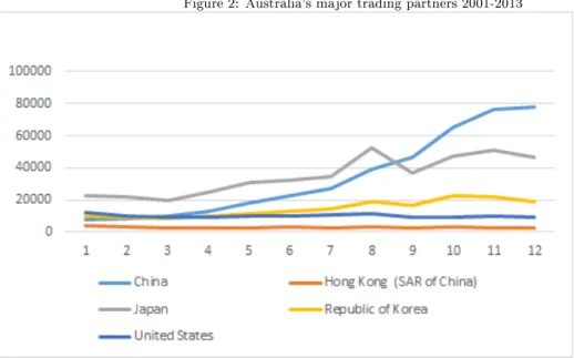
2 and Chinese markets, as represented by Hong Kong and the Hang Seng Index, not Shanghai and the Shanghai Composite Index, because the Spillover Index analysis, conducted in a VAR and variance decomposition framework, reveals that these two markets are the most inuential on the Australian market, even though they are currently ranked fourth and fth, in importance, as trading partners, (see Figure 2).
The recent GFC crisis commenced in 2007 and continued through to the European sovereign debt crisis. Alan Greenspan (2010) took the view that: The bubble started to unravel in the Summer of 2007. But unlike the debt-like deation of the earlier dotcom boom, heavy leveraging set o serial defaults, culminating in what is likely to be viewed as the most virulent nancial crisis ever. The major failure of both private risk management and ocial regulation was to signicantly misjudge the size of tail risks that were exposed in the aftermath of the Lehman default.
The U.S. subprime mortgage and credit crisis was characterized by turbulence that spread from subprime mortgage markets to credit markets more generally, and then to short-term interbank markets as liquidity evaporated, particularly in structured credit then on to stock markets globally. Gorton (2010) suggested that the GFC was not particularly dierent from previous crises except that, prior to 2007, most investors had never heard of the markets that were involved. Concepts such as subprime mortgages, asset-backed commercial paper conduits, structured investment vehicles, credit derivatives, securitization, or repo markets were not common knowledge. Gorton (2010) suggests that the securitized banking system is a real banking system that is still vulnerable to a panic. He argues that the crisis, beginning in August 2007, can best be understood as a wholesale panic involving institutions, where large nancial rms, "ran" on other nancial rms, making the system insolvent.
Fidrmuc and Korhonen (2010), analyze the transmission of global nancial crisis to business cycles in China and India using GDP data and dynamic correlation analysis. They report a sig-nicant link between trade ties and dynamic correlations of GDP growth rates in emerging Asian countries and OECD countries. Cheng, and Glascock (2005), examine the linkages among three Greater China Economic Area (GCEA) stock markets, including Mainland China, Hong Kong, and Taiwan, and two developed markets, Japan and the United States. They nd that a random walk model is outpredicted by an autoregressive GARCH model, and an ARIMA model, in all three GCEA markets, and that there is no evidence of cointegration between the markets. Chung et al. (2010), examine the informational role of the TED spread as perceived credit risk. They apply a Vector Autoregressive (VAR) model, Granger causality tests, cointegrating Vector Error Correction Model (VECM), to analyse the leadership of the US market with respect to UK, Hong Kong, Japan, Australia, Russia and China markets, during the crisis, and nd evidence of increased interdependence during the crisis. They suggest that the impact of orthogonalized shocks from the US market, on other global markets, increases by at least two times during the crisis, and that of the TED spread, even more so.
Didier et al. (2012), examine the determinants of comovement in stock market returns during the 20072008 crisis. They explore the inuence of the United States (US), via analysis of the factors driving the comovement between US stock market returns and stock market returns in 83 countries. Their analysis distinguishes between the period before and after the collapse of Lehman Brothers, and their ndings indicate that comovement was driven largely by nancial linkages. Dooley and Hutchison (2009) explore the transmission of the crisis to the emerging markets. They suggest that whilst initially these markets were largely shielded from the deleterious eects on world trade ows, they subsequently had strong eects after the Lehmann bankruptcy. Huang et al. (2000), apply similar causality and cointegration relationships among the stock markets of the United States,
3 Japan and the South China Growth Triangle (SCGT) region, and report no evidence of cointegration amongst these markets, save the Chinese ones of Shanghai and Shenzen. Kotkatvuori-Örnberg et al. (2013), explore stock market correlations during the nancial crisis across 50 equity markets. They measure the value of covariance information using an the augmented DCC model, and show that by taking into account the change in the level of variance in high volatility periods, the estimates of the conditional covariance are more ecient in capturing the dynamics of the stock market's variance. Min and Hwang (2012), also use dynamic correlation analysis of US nancial crisis to explore contagion from the US across four OECD countries. They nd a process of increasing correlations (contagion), in the rst phase of the US nancial crisis, and an additional increase of correlations (herding), during the second phase of the US nancial crisis, for the UK, Australia and Switzerland. Mun and Brooks (2012) explore the roles of news and volatility in stock market correlations during the global nancial crisis. Their results show that the majority of the correlations are more strongly explained by volatility than news. Yeh and Lee (2000), analyse the interaction and volatility asymmetry of unexpected returns in the greater China stock markets. They suggest that results, of a near vector autoregressions (VAR) model, reveal that the Hong Kong stock market plays an inuential role as a regional force amongst the Taiwan, Shanghai, and Shenzhen B-share stock markets.
There are a number of common themes in this literature. The global studies that include the US suggest that it has a major inuence in the transmission of shocks to both developed and undeveloped markets. The econometric methods, used in these studies, range across a number of time series econometrics techniques including cointegration, VAR models, and applications of models nested in the GARCH framework, including multivariate models such as DCC.
However, also germane to the approach adopted in the current paper, is a recent study by Diebold and Yilmaz (2009), who formulate and examine precise and separate measures of return spillovers and volatility spillovers. They base their measurement of return and volatility spillovers on vector autoregressive (VAR) models, in the broad tradition of Engle et al. (1990). They focus on variance decompositions, which they argue are well understood and widely calculated. They use them to aggregate spillover eects across markets, which permits the distillation of a wealth of information into a single spillover measure. We adopt their approach, plus a tri-variate Cholesky-GARCH model which permits an analysis of the relationships with those markets with the greatest inuence on the Australian market, as revealed by the application of their Spillover Index.
Our analysis is therefore focussed on the relationship with Australia's main trading partners, China, Japan, the United States, Hong Kong and Korea, given that both trade ows and attached information ows are likely to have an economic impact, and be reected in the behaviour of equity indices (see for example, Evans and Hnatkovska (2014)).
In this paper we focus on how the GFC impacted on volatility spillovers across the world to the Australian equity market. Even though the Australian nancial markets were spared the major eects of the GFC, in terms of distress to major nancial institutions, the Australian nancial market was still impacted by these major global events. The degree to which the Australian market is inuenced by extreme events in the US, has implications for portfolio optimization by Australian investors and fund managers alike, and eects the degree to which it is possible to hedge risk during times of nancial turbulence. We examine how both return and volatility spillovers and correlations changed, between the Australian market and the US during the nancial crisis. We focus on the impact of the Chinese market in our analyses, given that its is Australia's main trading partner, together with the inuence of the US market, given that this it has consistently been shown to have the greatest impact on other global markets, in the prior studies mentioned, even though it is only
4 Australia's fourth most signicant trading partner.
2. Research Method
2.1. Data set and econometric models
We wanted to make sure that we captured the relationships with Australia's main trading partners. Figure 1 below depicts Australia's top ten partners in trades in goods and services in 2013 taken from the DFAT top ten list.
Figure 1: Top 10 partners in trade in goods and services 2013
Source: http://dfat.gov.au/publications/tgs/index.html
Figure 2 depicts the trend in trade in goods and services from 2001 to 2013, with exports in the top half of the diagram and imports in the bottom. It can be seen that trade with China has become ever more important overtaking trade with Japan as the major trading partner in 2008-2009. Trade with Korea, particularly in imports, has increased in importance since 2004 when it overtook trade with the US in relative importance. The fth most important trading partner is Hong Kong whose relative importance has not changed over this period. For the purposes of our analysis we have concentrated on the top six trading partners, in terms of exports, as this reects our major trading partners and has implications for export income.
2.1 Data set and econometric models 5
Figure 2: Australia's major trading partners 2001-2013
Source: Department of Foreign Aairs and Trade.
We took a series of major stock market indices representing these six countries; namely the Shanghai Stock Exchange (SSE) composite index, the Hang Seng Index, the Australian All Ordi-naries Index, the Nikkei 225 Index, the S&P500 Index and the Kospi Index. The data set includes daily data for each index from 1st January 2004, until 30th June 2014. The indexes are total market indexes, based on market capitalizations, and are taken from Datastream standardised in US dollar terms. Daily returns are calculated as follows:
yit=ln(pit)−ln(pit−1) (1)
The data sets used are shown in Table 1. (We lagged the US S&P 500 index returns by one day to make them more comparable in time with the Australian and other Asian series).
Country Index
USA S&P500
AUSTRALIA All Ordinaries
CHINA Hang Seng
CHINA Shanghai Stock Exchange Composite
JAPAN Nikkei 225
KOREA Kospi
Table 1: List of countries and indices
There are a variety of models that could be used to test for the existence of time-varying volatility, and for spillover eects in returns and volatility across markets.
2.2 The Diebold and Yilmaz (2009) Spillover Index 6 One approach is to use a time series Vector Autoregressive (VAR) framework. This was recently formalised by Diebold and Yilmaz (2009) and Diebold and Yilmaz (2012), who modelled spillovers using VAR models and variance decompositions. They constructed a spillover index based both on return spillovers and volatility spillovers. Their approach is initially attractive for our purposes, because it enables us to see which of the six markets considered makes the largest contribution to the spillover of returns and volatilities into the Australian market. We commence with an application of their model which enables us to determine which of Australia's trading partners contributes most to equity shocks. Once we have used their model as an initial lter we then proceed to apply models within a GARCH framework.
The returns spillover index uses our basic index data. For the volatility based estimates we departed from the procedure used by Diebold and Yilmaz (2009), which used weekly ranged-based estimates to assess volatility. We preferred to use realised volatility metrics. We employ the the Oxford-Man Institute of Quantitative Finance's "realised library" which contains daily non-parametric measures of how the volatility of nancial assets or indexes were in the past. Each day's volatility measure depends solely on nancial data from that day. We choose the series constructed by sampling at 10 minute intervals within the day. Data is available for download on the Oxford-Man website (http://realized.oxford-man.ox.ac.uk/), and we took daily estimates for all our markets which were available for the full sample period, apart from the Shanghai Stock Exchange composite index which is not covered. The raw high frequency data is taken from Reuters DataScope Tick History database. These RV estimates were then utilised for the spillover index analysis of volatility. 2.2. The Diebold and Yilmaz (2009) Spillover Index
Diebold and Yilmaz (2009) suggest that the advantage of the adoption of a VAR framework and the use of variance decompositions is that they permit the aggregation of spillover eects across markets, distilling a wealth of information into a single spillover measure. This suits our current purposes and permits an examination of the relative contributions to spillovers made by the six markets in our sample. They proceed to develop their measure by taking each asseti, and adding the shares of its forecast error variance coming from shocks to assetj,for allj6=i, all in the context of an nvariable VAR. They then sum these error variances across all i = 1, ...., N.If we take the case of a covariance stationary, rst-order, two variable VAR, we have;
xt= Φxt−1+εt
wherext= (x1t, x2t)andΦis a 2×2 parameter matrix. In the empirical analysis which follows,
x will be either a vector of index returns or a vector of index volatilities. The moving average representation of the VAR can be written, given the existence of covariance stationarity, as;
xt= Θ(L)εt
whereΘ(L) = (1−ΦL)−1. The moving average representation can be conveniently written as;
xt=A(L)ut
where A(L) = Θ(L)Q−t1, ut = Qtεt,E(utu
0
t) = I, and Q
−1
t is the unique lower-triangular
Choleski factor of the covariance matrix ofεt.
Diebold and Yilmaz (2009) then proceed to consider the optimal 1 step ahead forecast, given by;
2.3 GARCH models 7
xt+1,t= Φxt,
with the corresponding one-step ahead error vector et+1,t=xt+1−xt+1,t=A0ut+1= a0,11 a0,12 a0,21 a0,22 u1,t+1 u2,t+1
which has the covariance matrix;
Eet+1,te 0 t+1,t =A0A 0 0
This suggests that the variance of a one-step ahead error in forecastingx1,tisa20,11+a20,12 and the variance of the one-step ahead error in forecasting x2,t is a20,21+a20,22. Diebold and Yalmiz (2009) demonstrate that it is possible to to split the forecast error variances of each variable into components attributable to the various system shocks. In this two variable system it is possible to distinguish between shocks to the variable itself xi and shocks to the other variable xj, for
i, j = 1,2,i6=j.
Diebold and Yalmaz calculate a spillover index in the two variable case as; S= a 2 0,12+a22,1 trace(A0A 0 0 ×100 (2)
They then generalise the measure to take into account multiple securities and multiple periods as shown below: S= PH−1 h=0 PN i,j=1 i6=j a2 h,ij PH−1 h=0 trace(AhA 0 h) (3) Diebold and Yilmaz (2012) extend their approach to include a generalized vector autoregressive framework in which forecast-error variance decompositions are invariant to variable ordering. We also apply this metric, but will not develop their model here, and refer the interested reader to their original discussion of the model (See Diebold and Yilmaz (2012)).
In the empirical work that follows in the next section, we will use second-order six variable VARs with 10 step-ahead forecasts, and apply the two variants of their model, to both return and variance series. The results suggest that the US market dominates spillovers, with the Hong Kong market the second most important from those considered. We use this nding in the subsequent GARCH analyses.
2.3. GARCH models
Manganelli and Engle (2001), claim that the main dierences between the variations in the approaches, adopted in this class of models, is how they deal with the return distribution, and they proceed to classify these models into three distinct groups:
Parametric, such as RiskMetrics and GARCH;
Nonparametric, such as Historical simulation and the Hybrid Model;
Semiparametric, such as CAViaR, Extreme Value Theory, and Quasi-Maximum Likelihood GARCH.
2.3 GARCH models 8 Engle (1982), developed the Autoregressive Conditional Heteroskedasticity (ARCH) model, that incorporates all past error terms. It was generalised to GARCH by Bollerslev (1986), to include lagged term conditional volatility. In other words, GARCH predicts that the best indicator of future variance is the weighted average of long-run variance, the predicted variance for the current period, and any new information in this period, as captured by the squared residuals (Engle, (2001)).
The framework is developed as follows: consider a time seriesyt=Et−1(yt)+εt,whereEt−1(yt)is the conditional expectation ofytat timet−1 andεtis the error term. The basic GARCH model
has the following specication:
εt= p htηt, ηt ∼N(0,1) (4) ht=ω+ p X j=1 αε2t−j+ q X j=1 βjht−j (5)
in which ω > 0, αj ≥ 0 and βj ≥ 0, are sucient conditions to ensure a positive conditional
variance, ht ≥0. The ARCH eect is captured by the parameter αj, which represents the short
run persistence of shocks to returns. βj captures the GARCH eect, and αj +βj measures the
persistence of the impact of shocks to returns to long-run persistence. A GARCH(1,1) process is weakly stationary ifαj+βj≤1.
Ling and McAleer (2003), and Harris, Stoja and Tucker (2007), claim that the GARCH model is perhaps the most widely used approach to modeling the conditional covariance matrix of returns. Engle (2001), states it has been successful, even in its simplest form, in predicting conditional variance. The main advantage of this model is that it allows; a complete characterization of the distribution of returns and there may be space for improving their performance by avoiding the normality assumption (Manganelli and Engle, (2001, p.9)). However, Engle (2001), Nelson (1991), Zhang and Li (2008), and Harris, Stoja and Tucker (2007), also outline some of the disadvantages of the GARCH model as follows; GARCH can be computationally burdensome and can involve simultaneous estimation of a large number of parameters. GARCH tends to underestimate risk, (when applied to Value-at-Risk, VaR), as the normality assumption of the standardized residual does not always hold with the behaviour of nancial returns. The specication of the conditional variance equation and the distribution used to construct the log-likelihood may be incorrect. GARCH rules out, by assumption, the negative leverage relationship between current returns and future volatilities, despite some empirical evidence to the contrary.
GARCH assumes that the magnitude of excess returns determines future volatility, but not the sign (positive or negative returns), as it is a symmetric model. This is a signicant problem, as research by Nelson (1991), and Glosten, Jagannathan and Runkle (GJR) (1993), shows that asset returns and volatility do not react in the same way for negative information, or `bad news', as they do for positive information, or `good news', of equal magnitude.
In order to deal with these problems, a large number of variations on the basic GARCH model have been created, each one dealing with dierent issues. Bollerslev (1990) developed a multivari-ate GARCH (MGARCH) model that asumes Constant Conditional Correlation (CCC). In other words, it assumes the independence of asset returns' conditional variance. Multivariate GARCH (MGARCH) models have recently been used widely in risk management and sensitivity analysis.
Bauwens, Laurent and Rombouts (2003), suggest that the most appropriate use of multivariate GARCH models is to model the volatility of one market with regard to the co-volatility of other markets. In other words, these models are used to see if the volatility of one market leads the
2.4 Multivariate conditional volatility models 9 volatility of other markets (the `Spillover Eect'). They also assert that these models can be used to model the tangible eects of volatility, such as the impact of changes in volatility on exports and output growth rates. Bauwens, Laurent and Rombouts (2003), suggest that these models are also ecient in determining whether volatility is transmitted between markets, through the conditional variance (directly), or conditional covariances (indirectly), whether shocks to one market increase the volatility of another market, and the magnitude of that increase, and whether negative information has the same impact as positive information of equal magnitude.
Nelson (1991) developed the Exponential GARCH (EGARCH) model. This model uses loga-rithms to ensure that the conditional variance is non-negative, and captures both the size and sign eects of shocks, capturing the eect of asymmetric returns on conditional volatility. This model was the rst to capture the asymmetric impact of information. A second model, which is computa-tionally less burdensome then Nelson's EGARCH, is the Glosten, Jagannathan and Runkle (GJR) model (1993). They found signicant evidence of seasonal eects on the conditional variance in the NYSE Value-Weighted Index. Engle and Ng (1993), claim that the GJR forecasts of volatility are more accurate than those of the EGARCH model. Necessary and sucient conditions for the second order stationarity of the GARCH model are Pr
i=1 αi+ s P i=1 βi<1, as demonstrated by Bollerslev
(1986). The necessary and sucient conditions for the GJR (1,1) model were developed by Ling and McAleer (2003), who showed thatE(ε2
t)<∞ if α1+γ21 +β1<1. Subsequently, McAleer et al. (2007) demonstrated the log-moment condition for the GJR(1,1) model, which is sucient for consistency and asymptotic normality of the QMLE, namely E(log(α1+γ1I(ηt)η2t +β1))<0. 2.4. Multivariate conditional volatility models
There are a wide variety of specications available for multivariate conditional volatility mod-elling. We originally adopted a bi-mean equation to model the conditional mean in the individual markets plus an ARMA model to capture volatility spillovers from the US across the other markets considered. We commenced by adopting a vector ARMA structure with exogenous variables for the conditional mean equationµt as shown below:
ut= Υxt+ p X i=1 Φirt−i− q X i=1 Θiat−i (6)
wherext denotes an m-dimensional matrix of explanatory variables,Υis ak×mmatrix andp
andqare nonnegative integers.
We considered univariate models of single assets in the previous section. However, in nance the behaviour of portfolios of assets is of primary interest. If we want to forecast the returns of portfolios of assets, we must consider the correlations and covariances between individual assets. A common approach adopted to the specication of multivariate conditional means and conditional variances of returns is as follows:
yt=E(yt|Ft−1) +εt (7) εt=Dtηt In (5) above,yt= (y1t, ..., ymt) 0 , ηt = (ηit, ..., ηmt) 0
, a sequence of (i.i.d) random vectors, Ft is a vector of past information available at time t, Dt = diag(h
1/2
1 , ..., h
1/2
2.5 Model specications 10 number of returns, and t = 1, ...., n. (For a full exposition, see Li, Ling and McAleer (2003), McAleer (2005) and Bauwens et al (2003). The Bollerslev (1990) constant conditional correlation (CCC) model assumes that the conditional variance of each return, hit, i = 1, ...., m, follows a
univariate GARCH process:
hit=ω+ r X j=1 αijε2i,t−j+ s X j=1 βijhi.t−j (8)
In (6) above,αij represents the ARCH eect, or the short run persistence of shocks to returni,
andβij captures the GARCH eect; the impact of shocks to returnion long run persistence, given
by: r X j=1 αij+ s X j=1 βij.
It follows that the conditional correlation matrix of CCC isΓ =E(ηtη
0 t|Ft−1) =E(ηtη 0 t),where Γ ={ρit}fori, j= 1, ...., m.From (5),εt 0 t=Dtηtη 0 tDt, Dt= (diagQt)1/2, andE(εtε 0 t|Ft−1) =
Qt = DtΓDt, where Qt is the conditional covariance matrix, Γ = Dt−1QtDt−1is the conditional
correlation matrix and the individual conditional correlation coecients are calculated from the standardised residuals in equations (5) and (6). This means that there is no multivariate estimation required in CCC, which involvesmunivariate GARCH models, except in the case of the calculation of conditional correlations.
We initially attempted to apply variants of the VARMA-GARCH models but had diculty obtaining convergence and sensible results. We then decided to utilise Cholesky-GARCH decom-positions, in which the analysis is done sequentially, and avoided the problems with convergence using this approach. This could also be justied because the Spillover Index analysis indicated the relative importance of shock contributions from the dierent markets.
2.5. Model specications
Our goal in this paper is to model spillover eects, and we adopt a variety of parametric tech-niques. We commenced our analysis with Diebold and Yilmaz (2009) spillover index applying a VAR approach. Then we moved to a GARCH modelling framework with the adoption of multivari-ate models. Problems encountered with variants of the VARMA-GARCH models lead to the use of a model in which we could order the choice of markets. We explore the relationship between Aus-tralia and the other two most important markets contributing spillovers, using a Cholesky-GARCH model for the empirical analysis. (See the discussion in Tsay (2005) and Dellaportos and Pourah-madi (2012)). (We used modied versions of Tsay's (2005) Rats code and Doans (2011) Rats code to undertake the analysis).
In the context of measuring asymmetric shocks and spillover eects, we proceed as follows: 1. First we apply the Diebold Yilmaz (2009) and (2012) variants of the Spillover Index to model
spillovers in both returns and volatilities.
2. This analysis reveals which market indices have the greatest impact in terms of spillovers of returns and volatilities into the Australian market. We use this information to construct the appropriate multivariate GARCH model.
3. We utilise Cholesky decompositions to build a higher dimensional GARCH model. We write the vector return series asrt=µt+αtand use a vector AR model for modelling the behaviour
11 First we build a univariate GARCH model of the US S&P500 index series.
Then we add the Australian S&P200 index series to the system, perform an orthogonal trans-formation on the shock process of the Australian return series, and build a bivariate volatility model for the system. The parameter estimates for the US model developed in step one can be used as staring values in the bivariate estimation.
Given that Australia is a major trading partner of China it is possible that links with the Chinese markets also impact upon volatility. A third component of the system is a Chinese index, in this case the Shang Hai Stock Exchange index. The shock process for this third return series is subjected to an orthogonal transformation and a three-dimensional volatility model is then constructed. Once again the parameter values from the bivariate system can be used as starting values.
The application of Cholesky decompositions to GARCH models is discussed in Tsay (2005), Chang and Tsay (2010) and Dellaportos and Pourahmadi (2011). This type of model is closely related to factor models; see for example, the discussion of orthogonal GARCH models in Alexander (2001). The advantage of the approach is that the multivariate conditional covariance estimation can be reduced to estimating the 3N parameters of univariate GARCH models and a few 'dependence' parameters. The advantage of this approach is that the Cholesky-GARCH models have correla-tion matrices that are time-varying, and can be more exible than Bollerslev's (1990) constant-correlation GARCH models. The main disadvantage of the approach is that the stocks have to be ordered to construct the model. However, given that we already know the relative importance of their shock contributions this is not such a drawback for our current purposes.
The results from the empirical application of these two dierent approaches and models are presented in the next section.
3. Empirical results 3.1. Data characteristics
The characteristics of the basic index series, used in our data set and presented in Table 2, suggest the existence of non-normality and fat tails. The Jarque-Bera Lagrange Multiplier test rejects the null hypothesis that the data are normally distributed: the p-values for all indexes above are zero. This is also evident from the skewness and excess kurtosis of the data. In order to estimate the parameters in the GARCH models, the Quasi-Maximum Likelihood Estimator (QMLE) will be used.
3.1 Data characteristics 12
S&P500 ret ALL Ord ret HANGSENG ret NIKKEI ret SHANGHAI ret KOSPI ret Mean 0.000207 0.000260 0.000224 0.000149 0.000220 0.000390 Prob. 0.383365 0.403931 0.446977 0.600047 0.474944 0.280398 Maximum 0.1095719593 0.0810922093 0.1340432034 0.1164424712 0.0901937935 0.2464004135 Minimum -0.0946951447 -0.1584914625 -0.1358877686 -0.1118564652 -0.0910142789 -0.2047944126 Skewness -0.339884 -0.995545 0.043335 -0.386103 -0.272083 -0.303964 Prob. 0.000000 0.000000 0.354947 0.000000 0.000000 0.000000 Excess Kurtosis 11.898603 9.782006 10.072437 6.134828 3.909530 20.087461 Prob. 0.000000 0.000000 0.000000 0.000000 0.000000 0.000000 Variance 0.000155 0.016900 0.000238 0.000220 0.000259 0.000358 Jarque-Bera 16198.34 11364.489773 11570.839096 4360.088133 1776.831001 46058.652729 Prob. 0.000000 0.000000 0.000000 0.000000 0.000000 0.000000
Table 2: Descriptive statistics
The two returns series are clearly non-normal as reected in the descriptive statistics reported in Table 2. Plots of the Index return series are shown in Figure 3.
Figure 3: Return Series plots for Australia, US, Japan, Hong Kong, Shanghai and Korea.
Plots of the Oxford-Man RV estimates, sampled at ten minute intervals within the day, and used as the series for our measures of index volatility are shown in Figure 4.
3.2 Spillover Index Results 13
Figure 4: Volatility Series plots for Australia, US, Japan, Hong Kong, and Korea.
3.2. Spillover Index Results
The results of the application of the Spillover index to the return series, and the various decomposition analyses, are shown in Table 3. One of the startling features of Table 3 is the degree of inuence on the Australian All Ordinaries returns series exerted by the other equity markets of its major trading partners. Its contribution from others' returns, presented in the extreme right hand column of Table 3, is the largest at 57%, whilst its contribution to its own return shocks, is the lowest at 42.9%. At the other extreme, the most independent market indices in Table 3, are the Shanghai composite, which explains 96.1% of the shocks to its own return series, and the S&P500 Index, which explains 99.6% of its own return shocks.
In terms of contributions to the behaviour of other markets return series, the least inuential is the Korean Kospi, which only contributes 1%, as can be seen in the penultimate row of the column headed by 'Kospi', in Table 3. The most inuential market is the US market, which contributes 117%. The Australian market contributes 10%, more than Japan, which contributes 6%, but less than the Hong Kong contribution at 37%, and Chinese contribution, via the Shanghai Composite, which contributes 25%. However, the bulk of Chinese inuence is on the Hong Kong Index, measured at 13.2%, and the Korean Kospi, recorded at 5.7%.
The two large inuences on the Australian All Ordinaries return series, which can be seen by looking across the row labelled 'All Ordinaries' in Table 3, are rst and foremost the US market, which contributes 41% on average, and the Hong Kong market, which contributes 11.7%. The inuence of the Shanghai Composite is only small measured at 3.6%. The relative inuence of the various markets considered in the analysis can be seen in the bottom row of Table 3. The most inuential is the US market, with a total contribution of 217%, if we include its contribution to its own variance. The next most inuential market is the Chinese market, via the Shanghai Composite, with a total contribution measured at 121%, but the bulk of this inuence is within it own borders, given that it contributes 13.2% to Hong Kong return behavior, and the rest largely impacts on the Korean market, which is recorded at 5.7%. There is only a small residual inuence on Australia and Japan at 3.6% and 2.2% respectively. Table 3 reects an average of the contributions over the entire sample period. A moving average analysis was also conducted.
3.2 Spillover Index Results 14
Table 3: Spillover Index variance decomposition of index returns
Shanghai Composite
Hang Seng All Ordinaries Nikkei S&P500 Kospi Contribution from others Shanghai Composite 96.1 0.0 0.2 0.5 3.1 0.1 4 Hang Seng 13.2 60.0 1.0 0.8 25.0 0.1 40 All Ordinaries 3.6 11.7 42.9 0.4 41.0 0.4 57 Nikkei 2.2 7.9 4.3 59.6 26.0 0.1 40 S&P500 0.0 0.1 0.1 0.1 99.6 0.1 0 Kospi 5.7 17.6 4.5 4.2 22.3 45.8 54 Contribution to others 25 37 10 6 117 1 196 Contribution including own 121 97 53 65 217 47 32.7%
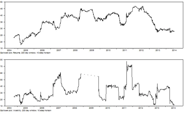
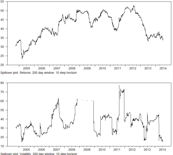
The rolling 200 period moving average of the contributions are shown in Figure 5. Figure 5: Moving average analysis of return and volatility spillovers using a 200 day window
The return spillover eects in the top panel of Figure 5 are smoother than the volatility spillover eects in the bottom panel. The return spillovers peak in 2008-2009 and in 2011-2012. The volatility spillover eects are not as smooth and peak in the middle of 2007, consistent with the onset of the GFC, and then again in late 2008-2009, before reaching an even higher peak in late 2011. The composition of the volatility spillover contributions is shown in Table 4.
3.2 Spillover Index Results 15
Table 4: Spillover Index variance decomposition of index volatilities
Hang Seng All Ordinaries Nikkei S&P500 Kospi Contribution from others
Hang Seng 60.6 2.9 3.1 33.4 0 39 All Ordinaries 6.1 57.9 4.4 31.3 0.3 42 Nikkei 1.0 1.2 93.2 4.6 0.0 7 S&P500 0.4 1.3 0.4 97.3 0.6 3 Kospi 1.1 1.0 1.6 10.1 86.2 14 Contribution to others 9 6 9 79 1 105 Contribution including own 69 64 103 177 87 21%
Consistent with the evidence on the return series shown in Table 4, the US market is clearly the most dominant, with a small 3% contribution from other markets in explaining the variance of its own variances, but with a dominant contribution to the others of 79%.The second most independent market is Japan, which has 7% explained by external shocks. The US has the greatest inuence on the Hong Kong market at 33.4%, closely followed by Australia at 31.3%.
Indeed, Australia is the most dependent market in terms of shocks to its volatility, given that own shocks explain on average 57.9% of the variances, whilst outside markets explain 42%. The second most inuential market on the Australian market volatility is Hong Kong, which explains 2.9% of Australian volatility. The least inuential market is Korea which contributes 1% of the shocks to the volatility of the other markets, followed in lack of importance by Australia, which contributes 6%.
However, the Choleski decomposition and variance decompositions, as undertaken in the Diebold and Yilmaz (2009) analysis, are inuenced by the order in which the variables are placed in the VAR. Diebold and Yilmaz (2012) update their method using a generalized vector autoregressive framework, in which forecast-error variance decompositions are invariant to variable ordering. They exploit the generalized (GIRF) VAR framework of Koop, Pesaran and Potter (1996) and Pesaran and Shin (1998), to construct their improved Spillover metric. In the additional analysis reported in Tables 5 and 6, and in Figure 6, we cross check our analysis applying the GIRF framework as used by Diebold and Yilmaz (2012).
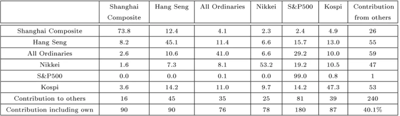
Table 5: Spillover Index GIRF variance decomposition of index returns
Shanghai Composite
Hang Seng All Ordinaries Nikkei S&P500 Kospi Contribution from others Shanghai Composite 73.8 12.4 4.1 2.3 2.4 4.9 26 Hang Seng 8.2 45.1 11.4 6.6 15.7 13.0 55 All Ordinaries 2.6 10.6 41.0 6.6 29.2 10.0 59 Nikkei 1.6 7.3 8.1 53.2 19.2 10.5 47 S&P500 0.0 0.0 0.1 0.0 99.0 0.8 1 Kospi 3.6 14.2 11.0 9.7 14.2 47.3 53 Contribution to others 16 45 35 25 81 39 240 Contribution including own 90 90 76 78 180 87 40.1%
3.2 Spillover Index Results 16 series. Australia is the most inuenced by external shocks to its return series, which explain 59% of its variance, whilst own shocks explain 41%. The most independent and inuential market is the US which contributes 81% of the shocks to other markets but explains 99% of its own variance. In terms of shocks to its returns, Australia is most inuenced by the US at a level of 29.2%, then by Hong Kong at 10.6%, followed by Korea at 10% and Japan at 6.6%. The least inuential series is that of the Shanghai Exchange, which contributes only 2.6%. China, in the form of the Shanghai Exchange, is the least inuential market in terms of the transmission of returns shocks, contributing only 16%, followed by Japan at 25% and then Australia at 35%. Hong Kong is the second most inuential market in the data set, contibuting 45% to the variance of returns in other markets.
The ordering of infuence does not correspond with market capitalizations. The NYSE has the largest current capitalisation in the World, followed by NASDAQ and then Japan. Hong Kong is the sixth largest market followed by Shanghai, then the Australian market is ranked fourteenth and the Korean market fteenth. The surprise, in this context, is the relatively small inuence of the Japanese market, event though it is the third largest in the world.
The relative rankings order is conrmed by the GIRF analysis of the variance Spillover Index shown in Table 6.
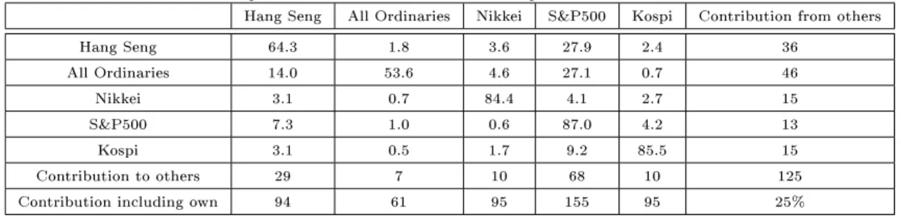
Table 6: Spillover Index GIRF variance decomposition of index variances
Hang Seng All Ordinaries Nikkei S&P500 Kospi Contribution from others
Hang Seng 64.3 1.8 3.6 27.9 2.4 36 All Ordinaries 14.0 53.6 4.6 27.1 0.7 46 Nikkei 3.1 0.7 84.4 4.1 2.7 15 S&P500 7.3 1.0 0.6 87.0 4.2 13 Kospi 3.1 0.5 1.7 9.2 85.5 15 Contribution to others 29 7 10 68 10 125 Contribution including own 94 61 95 155 95 25%
The GIRF analysis of Spillover variances, shown in Table 6, reveals that Australia is the least independent of all the markets, with own shocks explaining only 53.6% of its variances. The US market again has the greatest inuence, explaining 27.1% of the variances, followed by the Hong Kong market which explains 14% of the variances of the variances, and then the Japanese market, which explains 4.6%. In terms of contributions to explanations of the variances in volatility of other markets, the US market dominates, explaining 68% in total, followed by the Hong Kong market which explains 29%. The Australian market is the least inuential of those considered, and contributes only 7% to the explanation of the variances of the other markets considered.
3.3 Analysis within a GARCH framework 17
Figure 6: Moving average analysis of return and volatility GIRF based spillovers using a 200 day window
This analysis, using the Diebold and Yilmaz (2009) and (2012) versions of the Spillover Index, conrms that the Australian market is most inuenced by the US market, followed by the Hong Kong market. In the subsequent analysis, done withith a GARCH framework, we will concentrate on the contributions of these two markets.
3.3. Analysis within a GARCH framework
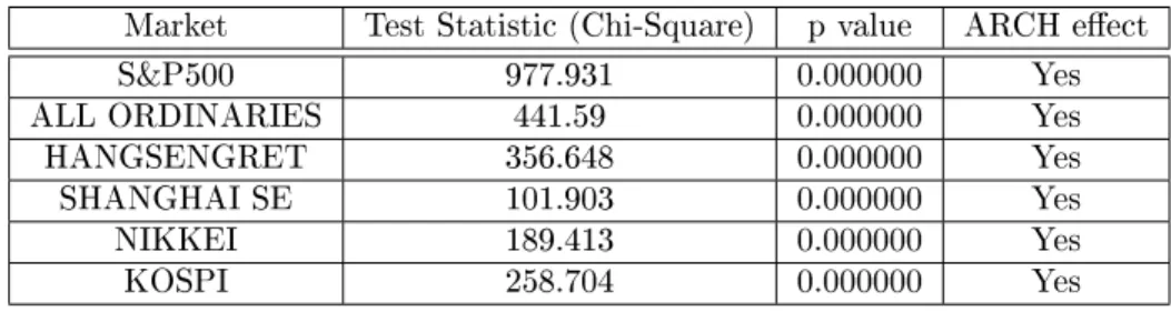
Before we conducted the GARCH tests, we tested for the existence of ARCH eects in the data sets. The results are shown below in Table 3, and display clear evidence of signicant ARCH eects in all of the index series.
3.4 Trivariate model based on Cholesky decompositions. 18 Market Test Statistic (Chi-Square) p value ARCH eect
S&P500 977.931 0.000000 Yes
ALL ORDINARIES 441.59 0.000000 Yes
HANGSENGRET 356.648 0.000000 Yes
SHANGHAI SE 101.903 0.000000 Yes
NIKKEI 189.413 0.000000 Yes
KOSPI 258.704 0.000000 Yes
Table 7: Test results for ARCH eects
The results in Table 3 mean we can proceed with condence to the GARCH analysis. 3.4. Trivariate model based on Cholesky decompositions.
We adopt a multivariate framework applying Cholesky-GARCH models. We estimate a uni-variate GARCH model for the US S&P500 index return series. We then add the Australian All Ordinaries index return series to the system, perform orthogonal transformation on the shock pro-cess for the Australian return series, and then build a bivariate volatility model for the system. We then augment the system further, and add in a return series for the Hang Seng Index to capture co-dependencies with China. The system then becomes a trivariate one.The parameter estimates for the GARCH model of the US return series are used as the commencement values in the bivariate estimation, and the estimation is augmented in a stepwise fashion, rst adding in the Australian index and then the Hang Seng index. The components of the return series are ordered as rt= (SP RET Lt, ASXRETt, HAN GSRETt). The sample means, standard errors and correlation
matrix of the data are:
ˆ µ= 0.00021 0.00026 0.00022 . ˆ σ1 ˆ σ2 ˆ σ3 = 0.0124 0.0163 0.0154 .ρˆ= 1.00 0.25095 0.22933 0.25095 1.00 0.65536 0.22933 0.65536 1.00 .
Tests of serial correlation in the three return series applying Ljung-Box statistics we obtain Q3(1) = 1205.43335, Q3(4) = 1280.38447, and Q3(8) = 1440.30046,and all are highly signicant with p values close to zero in terms of chi-squared distributions with 9, 36, and 72 degrees of freedom respectively. There is also signicant evidence of dependencies in cross-correlation matrices of returns up to six lags.
The initial estimate of the GARCH model for the US S&P 500 index return series yields the mean equation r1t = 0.00056169(0.00009224) +−0.0577rt−1(0.00531397) +a1t with signicance
levels in parentheses. The GARCH equation for the US S&P 500 index return series is h1t = 0.00000158(0.000) + 0.0862α(0.000) + 0.8987h1,t−1(0.000) +e1t. The system is then augmented by
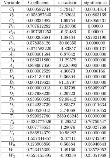
adding in the Australian S&P 200 index returns series. The model is re-estimated and nally the Hang Seng Index return series is added to the system. Our nal model is estimated as shown in Table 6.
Our nal mean equations are shown below:
rU SRET L,t=C1−P3U SRET Lt−1+a1t
rAU SRET ,t=C2+P21U SRET Lt−1−P22AU SRETt−1+a2t
rHAN GSEN GRET ,t=C3+P31U SRET Lt−1−P33HAN GSEN GRETt−1+a3t
3.4 Trivariate model based on Cholesky decompositions. 19 It can be seen in Table 6 that all coecients on lagged returns in the US market are signicant in all three mean equations and the lagged terms on the Australian and Chinese markets are also signicant in the mean equations. Manipulation of the above equations provides the three residual seriesa1t, a2t, a3t.
The three dimensional time-varying volatility model can be obtained as follows: g11,t=A0+A1b21,t−1+A2g11,t−1 q21,t=T0+T1q21,t−1−T2a2,t−1 g22,t=B0+B1b22,t−1+B2g22,t−1 q31,t=U0+U1q31,t−1+U2a3,t−1 q32,t=W0+W1q31,t−1+W2a2,t−1 g33,t=D0+D1b23,t−1+D2g33,t−1+D5g22,t−1 (10) Whereb1t=a1t, b2t=a2t−q21,tb1t, b3,t=a3,t−q31,tb1t,−q32,tb2t.
It can be seen in Table 6 that all terms exceptC3,D0,T2,U0,W0, W1,andW2,are signicant. Variable Coecient t statistic signicance
C1 0.000582744 3.79417 0.00014814 P3 -0.058987645 -2.62631 0.00863169 C2 0.000334982 1.69754 0.08959431 P21 0.707612282 32.85036 0.00000 P22 -0.097391253 -6.61486 0.00000 C3 0.000208681 1.08434 0.27821190 P31 0.578358126 30.06355 0.0000000 P33 -0.074583220 -4.83857 0.00000131 A0 0.000001584 6.87642 0.00000000 A1 0.086311860 11.29579 0.00000000 A2 0.898607050 102.85983 0.00000000 B0 0.000002529 4.30673 0.0000166 B1 0.081139161 9.36304 0.00000000 B2 0.900419623 81.19797 0.00000000 D0 0.000000013 0.03799 0.96969907 D1 0.037988239 6.29223 0.00000000 D2 0.930500532 92.98412 0.00000000 D5 0.024232739 3.85372 0.00011634 T0 0.000530013 3.74068 0.00018352 T1 0.999027780 2380.65243 0.00000000 T2 -0.034777026 -0.29552 0.76759547 U0 0.007778653 1.28076 0.20027768 U1 0.886814379 10.98282 0.00000000 U2 -1.557344857 -2.67711 0.00742597 W0 0.123906856 0.56884 0.56946643 W1 0.723415309 1.49166 0.13578952 W2 -0.525155895 -0.93358 0.35051968
20 The model diagnostics appear to be reasonably satisfactory, the Ljung-Box Q statistics for the three sets of residual series are insignicant for series RES1, RES2 and RES3 for 4, 8 and 12 lags respectively. There is evidence of an increased degree of correlation between the markets during and after the nancial crisis, as shown in Figure 6 below.
Figure 7: Time-varying correlations between the USA, Australia and China index series
The estimates in Table 6, of time varying correlations, augment the insights of the moving window estimates in Figure 5, of return and volatility spillovers across all three markets. There are peaks in correlations between the S&P500 and All Ordinaries Index, after the onset of the GFC, in 2008-2009, and then again in 2011. There is a low level of correlation between the S&P500 and the Hang Seng Index, but evidence of peaks in late 2008 and in 2011. There is a consistent and relatively high level of correlation between the Australian All Ordinaries and the Hang Seng Index, and evidence of peaks in late 2007, late 2008, 2010 and 2011.
4. Conclusion
This paper features an analysis of the impact of the GFC on Australian Index returns, and the transmission of volatility, from Australia's main trading partners to Australia, during this period. The Volatility Spillover Index analysis shows that the key inuences on Australia, in terms of both shocks to returns and to volatility, are the US and Hong Kong markets. Even though the Australian banking system faired well during the GFC, there is strong evidence of the transmission of volatility from the US to Australia, and to China, as reected in the behaviour of the Hang Seng index. However, there is little evidence of impact on Australian markets from China, as represented by the Shanghai market.
21 The trivariate Cholesky-GARCH model also shows strong inuence from US shocks on both Australia and China, though reduced inuence from China in the system. All correlations between the the three index series appear to rise post GFC.
The problems for investors in times of nancial crises appear to be exacerbated by the trans-mission of shocks; even countries that faired relatively well, such as Australia, were signicantly impacted. There is also less scope for risk diversication, as correlations appear to rise in times of nancial distress. Allen and Powell (2012) provide corroboratory evidence of the rise in riskiness of the Australian banks during the period of the GFC. Allen and Fa (2012), survey some aspects of the general impact of the GFC on Australian markets.
There is no obvious and straightforward interpretation of why some markets have more inuence on the Australian market than others. It is not a simple matter of market capitalisation, given that Japan ranks third in the World in terms of market capitalisation, and is ranked second as a trading partner to Australia, and yet has a relatively minor inuence on the Australian equity market. Hong Kong has a much greater impact, yet is only sixth in the world in market capitalisation terms, and is not as important as Japan, in trade terms. This issue merits further exploration.
22 [1] Allen, D.E. and R. Fa, 2012, The Global Financial Crisis: some attributes and
re-sponses, Accounting and Finance, Special Issue: Global Financial Crisis, 52, 1, 1-7. [2] Allen, D. E. and R.J. Powell, 2012, The Fluctuating Default Risk of Australian Banks,
Australian Journal of Management, 37(2), 297-325.
[3] Alexander, C. 2001, Market Models: A Guide to Financial Data Analysis, Wiley, New York.
[4] Barth, J.R., R. Koepp, and Z. Zhou, 2004, Banking Reform in China: Catalyzing the Nation's Financial Future, (2004) Available at SSRN: http://papers.ssrn.com/sol3/papers.cfm?abstract_id=548405.
[5] Bauwens, L., S. Laurent, and J.V.K. Rombouts, 2003, Multivariate GARCH models: A survey, CORE Discussion Paper No. 2003/31. Available at SSRN: http://ssrn.com/abstract=411062.
[6] Bollerslev, T., 1986, Generalized autoregressive conditional heteroscedasticity, Journal of Econometrics, 31, 307-327.
[7] Bollerslev, T., 1990, Modelling the coherence in short-run nominal exchange rates: A multivariate generalized ARCH model, Review of Economics and Statistics, 72, 498-505.
[8] Chang, C., and R.S. Tsay, 2010, Estimation of covariance matrix via sparse Cholesky factor with Lasso. J. Stat. Plan. Inference, 40, 3858 -3873.
[9] Cheng, H. and J. Glascock, 2005, Dynamic Linkages Between the Greater China Eco-nomic Area Stock MarketsMainland China, Hong Kong, and Taiwan, Review of Quantitative Finance and Accounting, 24, 343-357.
[10] Cheung, W., S. Fung, and S. Tsai, 2010, Global capital market interdependence and spillover eect of credit risk: evidence from the 20072009 global nancial crisis, Ap-plied Financial Economics, 20, 85-103.
[11] Dellaportos, P., M. Pourahmadi, 2012, Cholesky-GARCH models with applications to nance, Statistical Computing, 22, 849-855.
[12] Didier, T., I. Love, and M. Peria, 2012, What explains comovement in stock market returns during the 20072008 crisis? International Journal of Finance and Economics, 17, 182-202.
[13] Doan, T., 2010, RATS programs to replicate Diebold and Yilmaz EJ 2009 spillover calculations, Statistical Software Components from Boston College Department of Eco-nomics.
[14] Diebold, F, X., and K. Yilmaz, 2009, Measuring nancial asset return and volatility spillovers, with application to global equity markets, The Economic Journal, 158171. [15] Diebold, F. X., and K. Yilmaz, 2012, Better to give than to receive: Predictive direc-tional measurement of volatility spillovers, Internadirec-tional Journal of Forecasting, vol. 28(1), 57-66.
23 [16] Dooley M., and M. Hutchison, 2009, Transmission of the U.S. subprime crisis to emerg-ing markets: Evidence on the decouplemerg-ing-recouplemerg-ing hypothesis, Journal of Interna-tional Money and Finance, 28, 1331-1349
[17] Engle, R.F., 1982, Autoregressive conditional heteroskedasticity with estimates of the variance of United Kingdom ination, Econometrica, 50, 987-1008.
[18] Engle, R. F., 2001, GARCH 101: An Introduction to the Use of Arch/Garch Models in Applied Econometrics, Journal of Economic Perspectives,15, 4, 157-168.
[19] Engle, R.F., T. Ito, T. and W-L. Lin, 1990, Meteor showers or heat waves? Het-eroskedastic intra-daily volatility in the foreign exchange market, Econometrica, 58(3) (May), pp. 52542.
[20] Engle, R.F., V.K. Ng, 1993, Time-varying volatility and the dynamic behavior of the term structure, Journal of Money, Credit and Banking, 25 (3), 336-349.
[21] Evans, M.D.D., and V. V. Hnatkovska, 2014, International capital ows, returns and world nancial integration, Journal of International Economics, 92, (1), 14-33 [22] Gokcan, S., 2000, Forecasting volatility of emerging stock markets: linear versus
non-linear GARCH models, Journal of Forecasting, 19, 499-504.
[23] Gorton, G., 2010, Slapped by the Invisible Hand: The Panic of 2007, Oxford University Press, Oxford.
[24] Greenspan, A., 2010, The Crisis, Brookings Papers on Economic Activity, Spring. [25] Fidrmuc, J., and L. Korhonen, 2010, The impact of the global nancial crisis on
business cycles in Asian emerging economies, Journal of Asian Economics, 21, 293-303.
[26] Glosten, L.R., R. Jagannathan, D. Runkle, 1993, On the relation between the expected value and the volatility of the nominal excess return on stocks, Journal of Finance, 48, 1779-1801.
[27] Hamao, Y., R.W. Masulis, and V. Ng, 1990, Correlations in price changes and volatility across international stock markets, Review of Financial Studies, 3(2), 281-307. [28] Hamilton, J.D., 1989, A New Approach to the Economic Analysis of Nonstationary
Time Series and the Business Cycle, Econometrica, 57, 357-384.
[29] Harris, R.D.F., E. Stoja, J. Tucker, 2007, A simplied approach to modeling the co-movement of asset returns, Journal of Futures Markets, 27(6), 575-598.
[30] Harvey, C.R., A.R. Siddique, 1999, Autoregressive conditional skewness, Fuqua School of Business Working Paper No. 9604, Available at SSRN: http://ssrn.com/abstract=61332 or doi:10.2139/ssrn.61332.
[31] Huang B.-N., C-W.Yang, J.W.-S. Hu, 2000, Causality and cointegration of stock mar-kets among the United States, Japan and the South China Growth Triangle, Interna-tional Review of Financial Analysis, 9, 281-297.
24 [32] Johansson, A.C., and C. Ljungwall, 2009, Spillover eects among the Greater China
stock markets, World Development, 37, 4, 839-851.
[33] Koop, G., M.H. Pesaran, and S.M. Potter, 1996, Impulse Response Analysis in Non-Linear Multivariate Models, Journal of Econometrics, 74, 119147.
[34] Kotkatvuori-Örnberg, J., J. Nikkinen, and J. Äijö, 2013, Stock market correlations during the nancial crisis of 20082009: Evidence from 50 equity markets, Interna-tional Review of Financial Analysis,28, 7078.
[35] Lima, L.R., B.P. Neri, 2007, Comparing value-at-risk methodologies, Brazilian Review of Econometrics, 27(1), 1-25.
[36] Ling, S., and M. McAleer, 2003, Asymptotic theory for a vector ARMA-GARCH model, Econometric Theory, 19 (2), 280-310.
[37] McAleer, M., 2005, Automated inference and learning in modeling nancial volatility, Econometric Theory, 21, 232-261.
[38] McAleer, M., F. Chan, S. Hoti, and O. Lieberman, 2008, Generalized autoregressive conditional correlation, Econometric Theory, 24(6), 1554-1583.
[39] McAleer, M., F. Chan, and D. Marinova, 2007, An econometric analysis of asymmetric volatility: Theory and application to patents, Journal of Econometrics, 139, 259-284. [40] McAleer, M., S. Hoti, and F. Chan, 2009, Structure and asymptotic theory for
multi-variate asymmetric conditional volatility, Econometric Reviews, 28(5), 422-440. [41] Manera, M., M. McAleer, and M. Grasso, 2006, Modelling time-varying conditional
correlations in the volatility of Tapis oil spot and forward returns, Applied Financial Economics, 16(7), 525-533.
[42] Manganelli, S., and R.F. Engle, 2001, Value at risk models in nance, ECB Working Paper No. 75 Available at SSRN: http://ssrn.com/abstract=356220
[43] Min, H. and S. Hwang, 2012, Dynamic correlation analysis of US nancial crisis and contagion: evidence from four OECD countries, Applied Financial Economics, 22, 2063-2074.
[44] Moon G.H., and W.C. Yu, 2010, Volatility spillovers between the US and the China stock markets: Structural break test with symmetric and asymmetric GARCH ap-proaches, Glob. Econ. Review, 39(2), 129-149.
[45] Mun, M. and R. Brooks, 2012, The roles of news and volatility in stock market corre-lations during the global nancial crisis, Emerging Markets Review, 13, 1-7.
[46] Nelson, D.B., 1991, Conditional heteroskedasticity in asset returns: A new approach, Econometrica, 59(2), 347-370.
[47] Pesaran, M.H. and Y. Shin, 1998, Generalized Impulse Response Analysis in Linear Multivariate Models, Economics Letters, 58, 17-29.
25 [48] So, M.K., and A.S.L.Tsui, 2009, Dynamic modeling of tail risk: Applications to China,
Hong Kong and other Asian markets, Asia-Pacic Financial Markets,16, 183-210. [49] Tsay, R., 2005, Analysis of Financial Time Series, 3rd ed.Wiley, New York.
[50] Yeh Y.-H., T-S, Lee, 2000, The interaction and volatility asymmetry of unexpected returns in the greater China stock markets, Global Finance Journal, 11, 129-149.