Electricity Generating Portfolios with Small Modular Reactors
Geoffrey Rothwell, Ph.D., Stanford University (retired) [email protected] and Francesco Ganda, Ph.D., Argonne National Laboratory, [email protected] Nuclear Engineering Division, Argonne National Laboratory, Argonne, IL 60439-4814
May 2014
ABSTRACT
This paper provides a method for estimating the probability distributions of the levelized costs of electricity. These probability distributions can be used to find cost-risk minimizing portfolios of electricity generating assets including Combined-Cycle Gas Turbines (burning natural gas), coal-fired power plants with sulfur scrubbers, and Small Modular Reactors, SMRs. Probability densities are proposed for a dozen electricity generation cost drivers, including fuel prices and externalities costs. Given the long time horizons involved in the planning, construction, operation, refurbishment, and post-retirement management of generating assets, price data from the last half century are used to represent long-run price probabilities. This paper shows that SMRs can competitively replace coal units in a portfolio of coal and natural gas generating stations to reduce the levelized cost risk associated with the volatility of natural gas prices and unknown carbon costs.
Acknowledgements: US Department of Energy (Office of Nuclear Energy, DOE-NE) directly (ANL Contract #0F−34781) and indirectly through Argonne National Laboratory, ANL. We extend our thanks to M. Crozat, S. Goldberg, F. Lévêque, P. Lyons, H. Maertens, R. Rosner, G. Tolley, R. Vance, and seminar participants at the University of Chicago’s Harris School of Public Policy and the Energy Policy Institute at Chicago for their comments, encouragement, and data. Geoffrey Rothwell is currently working for the Nuclear Energy Agency of the Organization for Economic Cooperation and Development. This paper reflects the views of the authors, and not those of Stanford University, OECD-NEA, ANL, or US DOE.
Section 1: The Levelized Cost of Electricity
In the U.S. from the 1930s through the 1980s, electricity generating plants were built under either (1) some form of government or cooperative ownership, or (2) some form of private ownership with monopoly distribution rights and rate-of-return regulation. To satisfy growing demand, in a rate-of-return regulated utility or state-owned enterprise making the decision regarding what electricity generating technologies came down to the question: “What’s the cheapest?” During the last half century, a single economic metric has been employed to determine the projected costs of generating electricity: the levelized cost of electricity, LCOE. See definition of levelized cost in NEA-IEA (2010). The levelized cost methodology assigns all costs and revenues to years of construction, operation, and dismantling. Each cost in each year is discounted to the start of commercial operation at an appropriately weighted average cost of capital, such as 7.5%. The “levelized cost” is the tariff that equates the present values of investments, expenditures, and revenues, including a rate-of-return on both debt and equity.
However, ex ante when the levelized cost of a new technology is calculated, there are unknowns and uncertain variables in the calculation such as construction cost and duration, operating expenses, and fuel costs. Most calculations of levelized cost of electricity assume that each of the variables is represented by a single, best estimate, or a range of reasonable estimates. Unfortunately, given the uncertainty of future projections, a single best estimate for these variables is not likely to be as reliable as knowing a probability distribution for each of the cost drivers. This will allow the LCOE to be shown as a distribution that reflects these uncertainties.
Given the lengthy life times of electricity generators, constructing generating assets requires a long-term time horizon, something that is not necessarily built into unregulated electricity markets. As electricity markets deregulated, U.S. electric utilities moved toward natural gas, because during much of the day, natural gas prices set the marginal cost of electricity, hence its price in deregulated markets. If the producer is burning gas, it will at least do as well as the rest of the sellers of electricity from natural gas. But this “dash to gas” also led to volatile electricity prices, following price volatility in the natural gas market. The cost structure of generating electricity from natural gas leaves it particularly susceptible to this volatility because it is the technology with the highest share of its LCOE coming from fuel costs. Consumers must either accept this price risk or look to long-term bulk sales to reduce it.
Therefore, given the complexity of complete electricity markets and the lack of a long-term prospective in many of the remaining markets, there is a role for public policy in helping to encourage the building of portfolios of generating assets to (1) minimize total cost and cost risk, (2) minimize carbon dioxide emissions, and (3) maximize energy security for the nation through the diversification of electricity generation. This paper describes how to approximate the probability distributions of levelized cost drivers, how to simulate the levelized cost of electricity, and how to use these probability distributions to construct generating asset portfolios to minimize the cost risk associated with volatile energy prices, volatile weather conditions, volatile international energy markets, and volatile international relations.
The analysis relies on modern portfolio theory to provide a framework to investigate the risk-return tradeoffs of a portfolio of electricity generating technologies. Portfolio theory was developed in the 1950s to evaluate different combinations of financial assets (stocks, corporate
bonds, government bonds, etc.) to assess how the resulting portfolio would be expected to perform both in terms of likely returns, and the risks that the holder would have to bear. Portfolio theory has been the basis of financial planning for the last half-century, especially driving home the importance of having diversified portfolios to minimize risk while preserving returns. At the heart of this finding is that having assets that do not move together reduces volatility of the portfolio while preserving its expected long-term value (such as a portfolio of stocks with volatile returns and bonds with more stable returns). This paper applies the models that were developed to assess these financial tradeoffs to electricity generating portfolios. (For an application of real options theory to the choice of new nuclear in Texas, see Rothwell 2006.)
Because of the near lack of cost correlation between nuclear power and fossil-fired plants, nuclear power can balance the levelized cost of portfolios of fossil-fired power plants. Small Modular Reactors, SMRs, show promise in replacing coal units while natural gas prices are low and could be built to replace natural gas units as the price of natural gas rises.
This paper simulates the levelized costs of SMRs, Combined-Cycle Gas Turbines, CCGTs, burning natural gas, and coal-fired power plants with sulfur scrubbers, COAL (compare with Lévêque, 2013, pp. 48-60). Because the technology for producing energy is fixed during the life of the plant, total construction cost, KC, and hence, levelized capital cost, are fixed at the time of construction completion; capital additions are expensed in the levelized cost model and added to Operations and Maintenance costs, O&M. (Refurbishment costs are not included in this analysis.) Unless otherwise specified, all monetary values are in 2013 dollars. In this context, the levelized cost per megawatt-hour, MWh, can be defined as
LCk = [[FCR(r) · KC(OCk, r, ltk)] + FUELk(Fk, pFk) + O&Mk(Lk, pL)] / Ek , (1.1.1) where
k indicates the power generating technology, S for SMR, G for CCGT, or C for coal, etc.;
FCR is the Fixed Charge Rate (also known as the Capital Recovery Factor, CFR) is a function of the cost of capital, r, and the plant’s depreciation life,T:
FCR = [r (1 + r)T / [(1 + r)T – 1] ; (1.1.2)
KC(OCk, r, ltk) is the total construction cost, which is a function of the overnight cost, OCk (which is a function of the size of the plant, MWk), the cost of capital, r, and the lead time of construction, ltk; the product of FCR and KC yield a uniform annual payment to investors;
FUELk (Fk, pFk) is the annual fuel payment and a function of the amount of fuel, Fk, and price of fuel, pFk;
O&Mk (Lk, pL) is the annual Operations and Maintenance expense and a function of the amount of labor, Lk, and the price of labor, pL (which is assumed uniform across the generating industry); and
Ek = MWk · TT · CFk, (1.1.3) where MWk is the size of the power plant in megawatts, TT is the total time in hours in a year, and CFk is the power plant’s annual capacity factor. Capacity factors are discussed in Section 2.7 for nuclear power plants and in Section 3 for fossil-fired power plants. (Other operating modes, intermittent renewables, such as wind, will be added in future work.)
In Equation (1.1.1) some elements are considered parameters (and are represented in non-Italic fonts) and assigned specific values; the influence of these values is determined with sensitivity analysis. The parameters include (1) the cost of capital, r; (2) the life time of the plant, T; (3) the price of labor, pF ; (4) the size of the plant, MW; and (5) the total number of hours in a year, TT. The remaining elements are variables that can be functions of other parameters and other variables, such as in Equation (1.1.3), where the random variable Ek is a function of the parameters MW andTT and the random variable CFk. Using historic data, random variables are modeled with reasonable probability distributions. The probability distributions for the LCk in Equation (1.1.1) will be determined using a Monte Carlo process and compared with other generation technologies and in portfolios of electricity generators.
Section 2 discusses the parameters, variables, and levelized cost of Small Modular (Light Water) Reactors, SMRs, based on the costs of Advanced Light Water Reactors, ALWRs. Section 3 discusses the parameters, variables, and levelized cost of natural gas and coal-fired power plants. Section 4 calculates the expected levelized costs and standard deviations of portfolios of generating assets. Section 5 summarizes the conclusions.
Section 2: The Levelized Cost of Electricity of New Nuclear Power
This section provides a method for estimating the probability distributions of levelized costs of new nuclear power, in particular, SMRs. Although ALWRs will not be included in the portfolio analysis, SMR costs are derived from the costs of ALWRs, given that many of the SMRs under development are Light Water Reactor technologies. Section 2.1 discusses the appropriate cost of capital under different regulatory programs in the U.S., and how to calculate the accumulation of financing costs during construction. Section 2.2 discusses appropriate contingencies on cost estimates and argues that the cost engineering literature on contingency is compatible with setting the contingency based on the standard deviation of the cost estimate. (The Appendix extends this discussion and introduces the literature on portfolios of financial assets.) Section 2.3 estimates new nuclear’s total construction cost and shows that the estimated overnight cost of a new ALWR unit in the U.S. can be modeled with a probability distribution with a mode of $4,400/kW and a standard deviation of $460/kW. Section 2.4 introduces a “top-down” model of SMR levelized cost. Section 2.5 through Section 2.7, respectively, discuss new nuclear’s power fuel costs, Operations and Maintenance (O&M) costs, and new nuclear’s capacity factor. Section 2.8 presents estimates of the probability distribution of new nuclear’s levelized cost of electricity.
Section 2.1: The Cost of Capital and Interest During Construction
Various public policy instruments have been proposed to lower the cost of capital to investors in new nuclear. To determine the impact of these instruments on the cost of capital, this section discusses the results of a cash flow model to calibrate changes in the WACC, “Weighted Average Cost of Capital,” r, with US Government taxes and policy instruments. (Rothwell, 2011, pp. 88-91, provides a detailed discussion of the cash flow model that was used in MIT, 2003, University of Chicago, 2004, and MIT, 2009.) Based on this literature, in this paper, levelized cost will be calculated for real weighted average costs of capital, WACC, of
3%, appropriate for self-regulated, state-financed utilities (e.g., TVA, see OMB 1992 on financing government projects); this can be considered the baseline “risk-free” rate (because tariffs or taxes can be raised to pay investment costs);
5%, appropriate for state-regulated utilities with Construction Work in Progress, CWIP, financing with access to loan guarantees and production tax credits;
7.5%, appropriate for state-regulated utilities with Allowance for Funds Used During Construction, AFUDC, financing with access to loan guarantees and production tax credits; and
10%, appropriate for utilities in deregulated markets without access to loan-guaranteed financing or production tax credits.
The real weighted average cost of capital, r, will be set equal to each of these rates (3%, 5%, 7.5%, and 10%) for both nuclear and fossil-fired forms of electricity generation. Sensitivity analysis will be performed to determine the influence of the cost of capital on levelized costs.
To understand the relationship between the cost of capital, construction lead time, and compounding Interest During Construction, IDC, consider capital construction expenditures, discounted to the beginning of commercial operation, i.e., when sales and revenues start:
IDC =
CXt · OC [(1 + m) –t – 1], t = – lt, . . ., 0 (2.1.1) where (1) the CXt are construction expenditure percentages of overnight cost, OC, in month t, and (2) m the monthly weighted average cost of capital during construction, (1 + m) = (1 + r)1/12. In addition, the IDC factor, idc, is the percentage add-on for financing charges. Because IDC depends on the construction expenditure rate (how much is spent in each month), Equation (2.1.1) can be complicated because the expenditure rate is not the same over the construction period with smaller amounts being spent early to prepare the site, larger amounts being spent on equipment in the middle of the project, and smaller amounts being spent at the end on instrumentation, training, and fuel loading. For probability analysis, what is required is to calculate the percentage increase in the overnight cost due to project financing, equal to the IDC factor, as a transparent function of construction lead time and the cost of capital.Equation (2.1.1) becomes a straightforward calculation if the construction expenditures have a uniform distribution, such that CXt = 1 / lt: total overnight cost divided by construction lead time,lt. Then Equation (2.1.1) can be approximated (Rothwell, 2011, p. 35) as
IDC idcOC, where (2.1.2)
idc = [( m / 2) lt ] + [(m2 / 6) lt2] (2.1.3) The idc factor is a function of a parameter, m, and a random variable, lead time, lt. The random variable, lt, is modeled by fitting construction lead time data for recently completed units from IAEA (2013). Because it is unlikely that the distribution of lead times for new nuclear plants is symmetric, the exponential distribution is more suitable to mimic lead time probabilities:
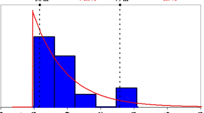
Exponential density: expo(b) = [exp( – x / b )] / b , (2.1.4a) Exponential distribution: EXPO(b) = 1 – exp( – x / b ) , (2.1.4b) where b and x must be greater than 0 (thus avoiding negative lead times in simulation), and b is equal to the mean and the standard deviation. Figure 2.1.1 presents construction lead time data in months fit to an exponential distribution. Because there is only one parameter in this distribution, a shift parameter is introduced to move the origin away from 0 months, this shift is added to b, yielding an expected mean of 59.26 months (= 11.75 + 47.51) or almost 5 years. Using this distribution implies that the construction lead time cannot be less than about 4 years, but could be greater than 10 years: there is no upper limit on construction lead time. (In the figures, blue represents input data, red represents probability densities, and purple represents both.)
It is assumed that the construction lead time for an SMR (Section 2.4) is one-half to two-thirds of that of an ALWR, i.e., an exponential distribution with a mean between 30 and 40 months with a standard deviation of 8 months. The Interest During Construction, idc, factor is simulated as in Equation (2.1.3). (Lead time only influences the idc factor in the model; overnight cost does not depend on the lead time, although Rothwell, 1986, found that construction cost was positively correlated with the construction lead time.)
Figure 2.1.1: ALWR Construction Lead Time in Months, Fitted to Exponential Density
Exponential[ 11.8 , Shift( 47.5)], Mean = 59 m, SDev = 10 m,Mode = 52 m
50 m 79 m 5.0% 19.1% 90.0%74.0% 5.0%6.9% 36 48 60 72 84 96 108 min =
Section 2.2: New Nuclear Power Plant Construction Cost Contingency
Traditionally, cost contingency estimation relied heavily on expert judgment based on various cost-engineering standards. Lorance and Wendling (1999, p. 7) discuss expected accuracy ranges for cost estimates: “The estimate meets the specified quality requirements if the expected accuracy ranges are achieved. This can be determined by selecting the values at the 10% and 90% points of the distribution.” With symmetric distributions, this infers that 80% of the cost estimate’s probability distribution is between the bounds of the accuracy range: X%.
To better understand confidence intervals and accuracy ranges, consider the normal (“bell-shaped”) probability distribution in Figure 2.2.1. The normal distribution can be described by its mean (the expected cost) represented mathematically as E(cost), and its standard deviation, a measure of the cost estimate uncertainty. The normal distribution is symmetric, i.e., it is equally likely that the final cost will be above or below the expected cost, so the mean equals the median (half the probability is above the median and half is below) and the mean equals the mode (the most likely cost). The normal density is
normal( , ) = (2 2 ) ½ · exp{ (1/2) · ( x )2 / 2 }, (2.2.1) where is the mean (arithmetic average), 2 is the variance, and is the standard deviation.
Figure 2.2.1 shows the normal density of a cost estimate with a mean, median, and mode of $1.5 billion and a standard deviation of 23.4%: 10% of the distribution is below $1.05B and 10% is above $1.95B, yielding an 80% confidence level.
Figure 2.2.1: A Generic Cost Estimate as a Normal Density
Normal ($1.5 B, $0.35 B), Mean = $1.5 B, SDev = 23.4% = $350 M
$0.50 $0.75 $1.00 $1.25 $1.50 $1.75 $2.00 $2.25 $2.50 in billions of $ 10% 10% 80% of the distribution is between $1.05 and $1.95 B = 1.5-(1.5 x 30%) to 1.5+(1.5 x 30%) Preliminary Estimate => 30%/1.28 = 23.4% Standard Deviation Standard Deviation= 23.4% x $1.5B = $0.35 billion 40% 40%
The cumulative distribution of the normal density, i.e., the normal distribution function,
NORMAL(, ), (which the integral of the area under the continuous red line in Figure 2.2.1) is not available in “closed form,” i.e., as a simple, algebraic equation (without integral calculus). The normal distribution function is shown in Figure 2.2.2 with non-symmetric distribution functions: the lognormal and the extreme value, discussed below):
lognormal( , ) = x1 (2 2 ) ½ · exp{ (ln x)2 / (2 · 2 ) }, (2.2.2) where is the mean and 2 is the variance; Johnson, Kotz, and Balkarishnan (1995).
Figure 2.2.2: Normal, Lognormal, and Extreme Value Distributions
0% 25% 50% 75% 100% $0.50 $0.60 $0.70 $0.80 $0.90 $1.00 $1.10 $1.20 $1.30 $1.40 $1.50 estimate in billions C u m u la ti v e P r o b a b il ity Lognormal (1.05, 0.18) Median at 50% 80% of distribution 10% 90% Extreme Value, maxv(0.95, 0.18) Normal(1.05, 0.23) Exponential [0.1, shift(0.6)]
If the cost estimate were normally distributed, the standard deviation would be
= X / Z , (2.2.3)
where X is the absolute value of the level of accuracy and Z depends on the confidence level. For example, the level of accuracy for a “Preliminary Estimate” is about 30%. If the cost estimator has an 80% confidence in this range of accuracy, Z = 1.28, i.e., 80% of the standard normal distribution is between the mean plus or minus 1.28 times . So, = (30% / 1.28) = 23.4%, which is in the range of 15-30% suggested in the literature, e.g., EPRI (1993). Also, the level of accuracy for a “Detailed Estimate” is about 20%. With the same level of confidence, Z = 1.28,
= 20% / 1.28 = 15.6%, which is in the suggested contingency range of 10-20%. Also, the level of accuracy for a “Final Estimate” is about 10%. With the same level of confidence, = 10% / 1.28 = 7.8%, which is suggested contingency range of 5-10%; see Rothwell (2005).
These guidelines suggest a “rule-of-thumb”: the contingency is approximately equal to the standard deviation of the cost estimate (and vice-versa, that the standard deviation of a cost estimate is approximately equal to the contingency):
CON|80% ≈ , e.g., 7.8%|±10%, 15.6%|±20%, or 23.4%|±30% . (2.2.4)
The Appendix (Section A1) discusses the appropriate risk aversion premium to place on the standard deviation of the cost estimate at different levels of confidence in the cost estimate. It finds that one cannot simultaneously determine the level of accuracy of the cost estimate, the level of confidence in the cost estimate, and the level of aversion to the standard deviation of the cost estimate. Therefore, a risk aversion parameter is set to 1.00, and multipliers are applied to to account for ranges of accuracy, levels of confidence, and aversion to risk (standard deviation).
Section 2.3: New Nuclear Power Plant Construction Cost
Construction Cost, KC, is the total amount spent on construction before any electricity or revenues are generated, as defined in Cost Estimating Guidelines for Generation IV Nuclear Energy Systems (EMWG, 2007) developed by the Economic Modeling Working Group of the Generation IV International Forum. KC is equal to total overnight construction cost plus contingency and financing costs. To measure these consistently, a set of standard definitions of construction accounts, structures, equipment, and personnel is required. Here, in the Code of Accounts, COA, from EMWG (2007), the total construction cost, KC, includes
(1) DIR: direct construction costs plus pre-construction costs, such as site preparation; (2) INDIR: the indirect costs;
(3) OWN: owners’ costs, including some pre-construction costs, such as site licensing, fee, including the environmental testing associated with an Early Site Permit and/or the Combined Construction and Operating License;
(4) SUPP, Supplemental costs (primarily first core costs; if first fuel core costs are levelized in the cost of fuel, as is done here, SUPP can be set to $0/kW);
(5) Contingency is expressed here as a contingency rate, CON; for example, 15%; and
(6) Interest During Construction, IDC, is expressed as a percentage markup on total overnight costs, (1 + idc), which is also known as the “IDC factor.”
Indirect costs can be expressed as a percentage markup, in, on direct cost: INDIR = in ∙ DIR. The indirect percentage markup, in, is set to 10% (EMWG 2007). Second, the owners’ costs associated with the development of the site, e.g., US NRC and US EPA licensing fees and site preparation expenses, are set to fee = $200 M plus 5% of direct costs (EMWG 2007). There is no indirect on owners’ costs.
The sum of these costs is the base overnight construction cost, BASE. The term overnight describes what the construction cost would be if money had no time value. Some references define “overnight cost” without contingency, and some references define “overnight cost” with contingency, as does US EIA (2013). To make this distinction, BASE excludes contingency and
OC includes contingency. OC plus Interest During Construction, IDC, equals total Construction Cost, KC. To summarize (where the subscript k refers to ALWRs),
OCk = [DIRk (1.05 + in) + fee] (1 + CON) or (2.3.1a)
DIRk = ( [OCk / (1 + CON)] − fee ) / (1.05 + in) (2.3.1b)
KCk = [DIRk (1.05 + in) + fee] (1 + CON) (1 + idck) (2.3.2) Concerning current estimates of new nuclear power plant construction costs, there is little publicly available data on expected costs for the nuclear power units under construction. However, there are estimates of total overnight costs for the Westinghouse AP1000s, because two twin AP1000s are under active construction with two more sites being prepared, and a version of the AP1000 is being built as two twin plants in China. There are a few construction cost estimates for twin AP1000s for the U.S.:
(1) There is the “certified cost” estimate for Vogtle Units 3 & 4: $4,418 M for a 45.7% share of 2,234 MW for Georgia Power (2010, p. 7). The Overnight Cost per kilowatt (including contingency, but not financing) is ($4,418 M/0.457)/(2.234 GW) = $4,330/kW. Updating this from 2010 dollars to 2013 dollars, yields $4,500/kW. (Although there has been some cost escalation during the construction of Vogtle, there is a conflict as to who will pay this increase; hence the amount of escalation will be unknown until the plant is completed.) (2) The SCE&G (2010, p. 3) overnight cost estimate for Summer Units 2 & 3 (= $4,270/kW/55%)/(2.234GW) = $3,475/kW in 2007 dollars, or $3,900/kW in 2013 dollars. (3) The Progress Energy overnight cost estimate for Levy County Units 1 & 2 is $4,800/kW in 2013 dollars, Progress Energy (2010, pp. 52-56, 132-140, and 320-321).
The average of these cost estimates is $4,400/kW (= $4,500+$3,900+$4,800/3) with a standard deviation of $460; as represented in Figure 2.3.1. In this paper, the baseline for ALWR construction cost is $4,400/kW in 2013 dollars. However, following Section 2.2, an appropriate contingency on overnight costs would be about 10.5% (= $460/$4,400) for 80% confidence, about 13.5% (= 1.29 · $460/$4,400) for 90% confidence, and about 16% (= 1.53 · $460/$4,400) for 95% confidence; see Table A1.1.
Figure 2.3.1: AP1000 Overnight Plant Costs, 2013$/kW, Fitted to a Normal Density
$3,000 $3,500 $4,000 $4,500 $5,000 $5,500 $6,000 2013 $ per kWe Summer Vogtl e Levy Turkey Point Range Normal($4,400, $460)
Mode = $4,400, Mean = $4,400, Median = $4,400, SDev = $460
Sources:Georgia Power (2010), SCE&G (2010), Progress Energy (2010), Scroggs (2010) To measure this uncertainty, there is a cost range for twin AP1000s in regulatory filings associated with Florida Power and Light’s Turkey Point Units 6 & 7. Also see Scroggs (2010, p. 45), “Updating the cost estimate range to 2010 dollars, adjusting for the 1,100 MW sized units a net 2.5% escalation rate, results in a cost estimate range of $3,397/kW to $4,940/kW.” This cost estimate range is $3,600/kW to $5,300/kW in 2013 dollars with a mid-point of $4,450/kW.
Following cost engineering guidelines (Section 2.2), if this range were expected to cover 95% of the realized Overnight Costs per kilowatt for Levy, the implied standard deviation would be $430/kW = ($850/1.96)/kW. The Levy cost estimate mid-point is only 1% different from the baseline here, $4,450/kW versus $4,400/kW. Because it is unlikely that the distribution of overnight costs for ALWRs is symmetric, the normal probability density of overnight costs is transformed into an extreme value density:
Extreme Value density: maxv(a, b) = (1/b) ∙ ab ∙ exp{ (– ab) } , (2.3.3a) Extreme Value distribution: MAXV(a, b) = exp{ – ab} , (2.3.3b) where ab = exp { – [(x – a) /b] }
and a is equal to the mode, and the standard deviation is equal to b times (π/√6) (≈ 1.28); Johnson, Kotz, and Balkarishnan (1995). The direction of the skewness in the extreme value distribution can be reversed, such that it has an extreme minimum value. This is designated here as minv(a, b) and MINV(a, b). With an extreme value distribution the expected overnight costs for twin ALWRs are shown in Figure 2.3.2, where the mode is equal to $4,400/kW, the mean is equal to $4,610/kW, and the standard deviation is equal to $460/kW (= $360 · π/√6)/kW.
Figure 2.3.2: ALWR Overnight Plant Costs, 2013$/kW, Fitted to an Extreme Value Density
Extreme Value, maxv($4,400, $360),
Mode= $4,400, Mean = $4,610, Median = $4,530, SDev = $460
$5,470
$4,000 90.0% 5.0%
$3,500 $4,000 $4,500 $5,000 $5,500 $6,000 $6,500
5.0%
Section 2.4: Small Modular Reactors
This section defines Small Modular Reactors, SMRs, as the term is used by the US DOE. In defining modular nuclear technologies, the term “module” has many meanings. The two most common usages of “module” in nuclear energy systems are (1) where equipment is delivered to the site as modules that can be plugged into one another and inserted into a structure with a minimum amount of labor, similar to “plug-and-play” personal computer equipment, and (2) where components and equipment of a nuclear power plant are made under factory quality-control, and delivered in a set of packages that can be assembled on-site, similar to home furniture. Here, (1) a “module” is a piece of pre-assembled equipment, e.g., the “reactor module;” (2) “modular construction” assembles factory-produced, pre-packaged structures on-site; and (3) “on-site construction” relies on site-delivered labor, machines, and materials to build structures and insert modules.
One or more SMR units make up an SMR plant. How unit costs change with reactor size is referred to as “scale economies” and can be represented with a scale parameter, S, such that cost declines (or increases) by (1 – S) for each doubling (or halving) of reactor capacity. For example, if S = 90%, then a 500 MW reactor would be 10% more costly than a 1,000 MW reactor, and a 250 MW reactor would be 23% more costly than a 1,000 MW reactor (from the same manufacturer) due to scale economies in reactor design of the same technology. (While there could be scale economies in the overnight cost of nuclear steam supply systems, because larger plants take longer to build, scale economies have not been detectable in total construction cost for nuclear power plants above 600 MW; Rothwell 1986.)
In Section 2.7, construction and levelized costs of twin 180 MW SMRs (the mPower design) are derived from construction and levelized costs of twin 1,117 ALWRs (the Westinghouse AP1000 design), assuming scale economies in reactor size, i.e., the larger the SMR, the lower the cost per kilowatt. (This analysis was easier when Westinghouse was actively working on an SMR and one could assume that the ALWR and SMR would be designed and built by the same manufacturer. So the scale relationship between reactors from different suppliers is only approximate.) On the other hand, transportation modes (e.g., rail cars) limit the size of the modules that can be shipped to a generic site. The stated sizes of the SMR reactor modules will vary as the designers minimize construction and other costs subject to manufacturing and transportation constraints.
To begin, the direct construction cost of a smaller reactor, DIRSMR, can be related to the cost for a larger reactor, DIRALWR, through set of multipliers, including a scale factor:
DIRSMR = DIRALWR (MWSMR / MWALWR) · S( ln MWSMR – ln MWALWR ) / ln 2, (2.4.1) where DIRALWRis from Equation (2.3.1b) and S is the scaling factor, e.g., 90%; see discussion of the “scaling law” in NEA (2011, p. 72). Although smaller in scale, SMRs are simpler in design with less equipment, reducing cost. Let s represent the factor saved by simplifying equipment in the design of the LWR SMR:
where s is the percentage reduction in cost associated with design simplification. If s were 85% (NEA, 2011, p. 75), direct costs would be 85% of what the costs would be in Equation (2.4.1).
Further, smaller reactors could enjoy economies of mass production (also known as serial economies or series economies, ser) over larger reactors, for example, in improved factory quality control, SMR direct costs could be lower than in Equation (2.4.2):
DIRSMR = DIRALWR (MWSMR/MWALWR) · ser · s · S(ln MWSMR – ln MWALWR) /ln 2, (2.4.3) where ser is the percentage reduction in cost associated with factory production, e.g., if ser were 15%, costs would be 85% of what the costs would be with Equation (2.4.2). In sum, SMR construction costs can be defined by Equation (2.4.3) and Equation (2.4.4):
KCSMR = [DIRSMR (1.05 + inSMR) + feeSMR] (1 + CONSMR) (1 + idcSMR) (2.4.4) Uniform probability distributions are assigned to ser [80%, 100%], s [75%, 95%], and S [80%, 100%] to simulate the probability distribution of KCSMR, as shown in Figure 2.4.1. (These parameters together can model most first- and second-order differences between ALWR and SMR costs.)
Figure 2.4.1: SMR Plant Overnight Costs 2013$/kW, Simulated, Fitted to a Lognormal Density
Lognormal[ $3,068, $864, Shift($1,434)], Mean = $4,500, SDev = $850, Median = $4,400
$6,000/kW $3,300/kW 5.0% 5.3% 90.0% 89.8% 5.0% 4.9% $2,000 $3,000 $4,000 $5,000 $6,000 $7,000 $8,000 $9,000
Source: Figure 2.3.2, Equations (2.4.3) and (2.4.4) with uniform distributions on ser, s, and S
Comparing Figure 2.3.2 and Figure 2.4.1 shows that the SMR overnight mean cost per MWh of $4,500/kW is between the mean and mode of the overnight cost of the ALWR, but the standard deviation (at this time) is nearly twice as high: compare the SMR standard deviation of $850/kW versus $460/kW for the ALWR. Also, Figure 2.4.2 presents a SMR construction lead time simulation as a function of the assumptions made in Section 2.1.
Figure 2.4.2: SMR Construction Lead Time, Simulated, Fitted to a Lognormal Density
Lognormal[ 14.0, 7.1, Shift(20.7)], Mean = 34.7 m, SDev = 6.9 m, Min = 24 m
49 months 26 months 5.0% 4.5% 90.0% 91.1% 5.0% 4.4% 20 25 30 35 40 45 50 55 60 65
Source: uniform distribution between 1/2 and 2/3 of those in Figure 2.1.1 Section 2.5: Nuclear Power Fuel Costs
Low Enriched Uranium, LEU, fuel accounting is complex if done precisely, i.e., by considering all lead and lag times of each fuel bundle from the first core through the last core. Here, as in most analyses, the assumption is that fuel is paid in a uniform stream over the life of the plant, without regard to the changing nature of a reactor’s set of irradiated fuel. This is similar to the assumption of leasing the fuel from a third party at a per-megawatt-hour fee. However, unlike carbon-fired plants, where fuel is expensed, nuclear fuel is capital that must be paid for over time. The cost of LEU is calculated using the formula from Rothwell (2011, p. 41). This cost includes the costs of natural uranium, conversion to uranium hexafluoride, enrichment, reconversion to uranium oxide, and fuel fabrication.
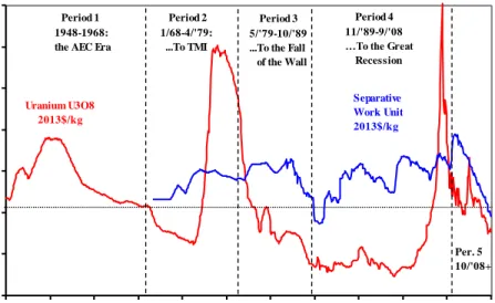
Figure 2.5.1 presents spot prices of uranium (in 2013 dollars per kilogram of uranium oxide, $/kg-U3O8) and the prices of enrichment, measured in Separative Work Units, SWU, in $/kg-SWU; prices have been converted using the monthly US Producer Price Index through 2013. Uranium prices from 1948 to 1972 are from US DOE (1981), converted to monthly prices by interpolation from mid-year to mid-year; prices from January 1973 through December 2006 are from Bureau of Agricultural and Resource Economics and Sciences (ABARES, 2007). Approximate prices since 2006 have been collected quarterly from the UXC website. For more information on uranium prices, see IAEA-NEA (2012).
In the U.S. market there have been five (illustrative) periods in the history of uranium prices.
Period 1 began in 1948 with purchases by the US Atomic Energy Commission, US AEC. Period 2 began in 1968 with private ownership of uranium in the U.S., but the US AEC maintained a monopoly on enrichment services. During this period, new private owners entered the market with little supply of uranium, driving up the price.
Period 3 began with the accident at Three Mile Island in April 1979, after which nuclear power plants under construction were cancelled and electric utilities left the uranium market; uranium prices fell almost continuously throughout the period; Rothwell (1980).
Period 4 began with the end of the Cold War, symbolically marked by the fall of the Berlin Wall, November 1989, and the entry of nuclear weapons highly enriched uranium into the market. The price of uranium hit historic lows before the possibility of a global nuclear renaissance pushed the price above its 1989 level in late 2003.
Period 5 has been a time of price instability with the end of surplus stockpiles, growth in nuclear power capacity in China and Korea, and the temporary shutdowns of nuclear power plants in Japan following the accident at Fukushima-Dai-Ichi in March 2011.
Figure 2.5.1: Natural Uranium and Separative Work Units, SWU, Spot Prices in 2013$/kg
$0 $50 $100 $150 $200 $250 $300 $350 1948 1954 1960 1966 1972 1978 1984 1990 1996 2002 2008 2014 $20 13/ k g Period 1 1948-1968: the AEC Era
Period 2 1/68-4/'79: ...To TMI
Period 3 5/'79-10/'89 ...To the Fall of the Wall
Period 4 11/'89-9/'08 …To the Great Recession Per. 5 10/'08+ Uranium U3O8 2013$/kg Separative Work Unit 2013$/kg
The annual prices of uranium and SWU from 1970 to 2014 were fitted to exponential and extreme value probability densities, respectively. Figure 2.5.2 presents annual uranium data fit to an exponential distribution, thus avoiding negative prices for natural uranium. Because there is only one parameter in this distribution, a shift parameter is introduced to move the origin above $0/kg, this shift is added to b, yielding an expected mean of $95.10/kg-U3O8 (= $69.60/kg + $25.50/kg). This limits values in the simulation of uranium prices to be above $25.50/kg-U3O8.
Figure 2.5.3 presents annual Separative Work Unit, SWU, prices fitted to an extreme value (minimum) distribution. While the mean of this distribution is $143/kg based on historic data, the price of Separative Work Units is now below $100/kg with the retirement of diffusion enrichment plants, and it is unlikely to rise above $143/kg (in 2013 dollars) due to excess capacity (particularly in Russia); see Rothwell (2009) and Rothwell (2012).
Figure 2.5.2: Natural Uranium 2013$/kg-U3O8 Prices, Fitted to an Exponential Density
Exponential[ $69.60, Shift($25.50)], Mean = $97,Median = $73,SDev = $74
$274/kg $33/kg 5.0% 2.8% 90.0% 86.9% 5.0% 10.3% $0 $50 $100 $150 $200 $250 $300 $350
Source: Annualized data from Figure 2.5.1
Figure 2.5.3: SWU 2013$/kg Prices, Fitted to an Extreme Value-Minimum Density
Extreme Value, minv($152.40, $17.59), Mean = $143, SDev = $20
$109/kg $167/kg 5.0% 8.1% 90.0% 81.6% 5.0% 10.3% $60 $80 $100 $120 $140 $160 $180 $200
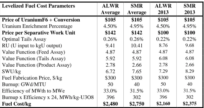
Table 2.5.1 specifies the baseline parameters for new nuclear fuel. Because of the historic stability, and little impact on the price of LEU, the price to convert U3O8 to UF6 is set at $10/kg and the fuel fabrication price to reconvert the UF6 to UO2 (metal) and to fabricate the UO2 into LEU fuel is set to $300/kg in 2013 dollars from the analysis in Rothwell (2010a). The cost of ALWR fuel is about $2,500/kg and the cost of SMR fuel is about $2,750/kg at a WACC of 7.5% (this rate discounts purchases of uranium and fuel services to the point when it is loaded into the reactor).
There are three primary differences between ALWR and SMR fuel: (1) in U.S. designs SMR fuel is enriched to just less than 5%, an US NRC threshold for Low Enriched Uranium, LEU, so the enrichment is slightly higher for SMRs than for ALWRs, requiring more Separative Work Units, SWU; (2) the burnup (B, in thermal gigawatt-days per tonne of uranium) is lower, e.g., 40 GWd/MTU, compared to 50 GWd/MTU, or higher, for ALWRs; and (3) the efficiency, ε, in converting thermal gigawatts into electrical gigawatts is lower for SMRs, for example, around 30% (here modeled with a uniform distribution between 30% and 33%), compared to around 33% for ALWRs. So, SMRs consume more uranium and SWU per MWh.
Table 2.5.1: Parameters for New Nuclear Fuel Cost Calculations (r = 7.5%)
Levelized Fuel Cost Parameters ALWR SMR ALWR SMR
Average Average 2013 2013 Price of UraniumF6 + Conversion $105 $105 $105 $105
Uranium Enrichment Percentage 4.50% 4.95% 4.50% 4.95%
Price per Separative Work Unit $142 $142 $100 $100
Optimal Tails Assay 0.26% 0.26% 0.22% 0.22%
RU (U input to kgU output) 9.41 10.41 8.76 9.68
Value Function (Feed Assay) 4.87 4.87 4.87 4.87
Value Function (Tails Assay) 5.92 5.92 6.08 6.08
Value Function (Product Assay) 2.78 2.66 2.78 2.66
SWU/kg 6.72 7.65 7.29 8.29
Fuel Fabrication Price, $/kg $300 $300 $300 $300
Burnup: GWd/MTU 50 40 50 40
Efficiency of MWth to MWe 33.0% 31.5% 33.0% 31.5%
Burnup x Efficiency x 24, MWh/kg-U3O8 396 302 396 302
Fuel Cost/kg $2,480 $2,750 $2,160 $2,375
If the price of SWU were $100/kg-SWU (the price has not been above $100/kg-SWU since 2013), fuel prices for ALWRs would be about $2,160/kg (a reduction of 13%) and fuel prices of SMRs would be about $2,375/kg (a reduction of 14%). Therefore, by maintaining the same methodology of modeling probability distributions for cost drivers based on historic data,
the price of LEU fuel is biased upward when compared to fossil-fired generators. (Also, back-end costs are assumed to be $0.85/kg for interim storage, see Rothwell, 2010b, and $1/MWh for geologic disposal.)
Section 2.6: Nuclear Power O&M Costs
Next, much has been written about the O&M costs of the currently operating PWRs and BWRs in the U.S. Unfortunately, the best data on nuclear power plant O&M costs are proprietary. Without access to these data, the following model is proposed: Labor, L, and Miscellaneous, M, costs are often grouped together in nuclear facility costs as Operations and Maintenance, O&M, costs where
O&M = ( pL ∙ L ) + M . (2.6.1)
Labor costs, pL ∙ L, are the product of (1) the average employee wages and benefits, and (2) the number of plant employees. Miscellaneous costs, M, include maintenance materials, capital additions, supplies, operating fees, property taxes, and insurance. Rothwell (2011, p. 37) estimates values for the amount of labor in Equation (2.6.1) using Ordinary Least Squares, OLS:
ln(L) = 5.547 + 0.870 (GW) , R2 = 96% (2.6.2)
(0.181) (0.099) Standard Error = 12.43%
where ln(L) is the natural logarithm of the number of employees and GW is the gigawatt size of the plant. In the semi-log form, the estimated constant is the minimum number of employees, i.e., exp[5.547] = 256 in Equation (2.6.2), and the estimated slope is the growth rate in employees with each GW increase in size. Equation (2.6.2) implies the staffing level for a 360-MW SMR would be about 350, or about 1 employee per 360-MW.
However, there is much less known about the standard error in applying the estimate in Equation (2.6.2) to SMR labor estimation. On the other hand, SMR labor should be lower per MWh than with ALWRs given the reduction in the complexity of the equipment. So, the standard error in simulation is modeled as a truncated normal with εL< 0. This reduces the level of employment by (on average) -9.6% (although it varies in simulation).
Assuming that the burdened labor rate, including benefits, pL, is $80,000 per employee per year in the U.S. (EMWG, 2007), the cost of fixed labor, LX, is
pL ∙ L = pL ∙ e5.55 ∙ e0.87 GW = $80,000 ∙ 350 ∙ (1 – 0.096) = $25 M . (2.6.3) Let the percentage markup, om, be 0.65, as in Rothwell (2011, p. 40), then
O&M = (1 + om) ( pL ∙ L ) = 1.65 ∙ $25 M = $41 M . (2.6.4) (In simulation, om varies between 0.55 and 0.75.) Dividing by expected MWh, as a function of the capacity factor (see the next section), the expected O&M cost per MWh is normally distributed with a mean of $15.69/MWh and a standard deviation of $1.39/MWh, as shown in Figure 2.6.1, modelled with a normal distribution in which 90% of the observations would be between $13/MWh and $18/MWh. These estimates are similar to those in Dominion Energy, Inc., Bechtel Power Corporation, TLG, Inc., and MPR Associates (2004).
Figure 2.6.1: Twin SMR O&M $/MWh, Simulated, Fitted to a Normal Density
Normal( $15.69, $1.39), Mean = $15.69,SDev = $1.39,Median = $15.83, Mode = $16.17
$13/MWh $18/MWh 5.0% 3.5% 90.0% 89.3% 5.0% 7.2% 10 12 14 16 18 20 22
Source: Equation (2.6.2) with a truncated normal error and Equation (2.6.4) Section 2.7: Nuclear Power Capacity Factors
The last random variable to discuss involves the denominator in Equation (1.1.1), as defined in Equation (1.1.3), where annual electrical energy output is a function of the size of the power plant, MW, the number of hours in a year, TT, and a random variable, CF, the capacity factor. The US NRC defines several capacity factors, each with a different measure of capacity. In Equation (1.1.3), let E be the NRC’s “Net Electrical Energy Generated” and MW be the “Net Maximum Dependable Capacity,” after subtracting power consumed by the plant itself. This is the most compatible with the IAEA’s definition of “Load Factor.” There are three related indicators of generating performance: productivity, availability, and reliability. (For a comparison of US NRC and IAEA definitions for these performance indicators, see Rothwell, 1990).
Productivity refers to the ability of the power plant’s generating capacity to produce electricity. Productivity is measured by the Capacity Factor, CFk, for each technology in each period. Let
CFkt Ekt / ( MWkt · TT ) . (2.7.1)
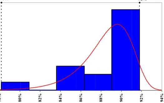
Figure 2.7.1 presents average annual capacity factors of U.S. nuclear power plants. These data are fitted to an extreme value density function with a mean value of 88.5% and a standard deviation of 2.5% with a minimum of 78.2% and a maximum of 91.8%.
Figure 2.7.1: U.S. Nuclear Power Plant Capacity Factors, Fitted to an Extreme Minimum Value Density
(annual average for the U.S. fleet of light-water nuclear power plants) Extreme Value, minv(89.6%, 2.5%), Mean = 89%, SDev = 3.3%,Min =78%, Max = 92%
78% 92% 5.0% 0.3% 90.0% 94.7% 5.0%5.0% 78% 80% 82% 84% 86% 88% 90% 92% 94% Source: http://www.eia.gov/totalenergy/data/monthly/pdf/sec8.pdf Section 2.8: New Nuclear Power’s Levelized Cost of Electricity
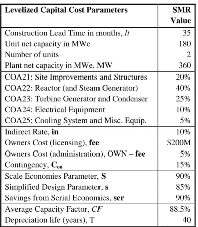
Table 2.8.1 presents parameters in calculating levelized capital costs for new nuclear. (Only Nth-of-a-Kind, NOAK, costs are considered here; on calculating First-of-a-Kind, FOAK, costs, see Rothwell, 2011, pp. 57-61.) (1) The first set of parameters specifies the size of the unit, the plant, and the typical number of units per plant. (2) The second set specifies the percentage allocations of direct construction expenditures for Code of Accounts (COA) 21-25; see EMWG (2007). Because these percentages are assumed the same for both ALWRs and SMRs, the cost of the reactor is the same proportion of direct costs for both technologies. (3) The third set of parameters specifies rates to transform direct costs into overnight costs, where a 15% contingency implies a “Detailed Estimate.” (Contingency was included in the observations on costs in Section 2.3, therefore the contingency here is associated with the uncertainty of building the same technology at a different site; note this upwardly biases the cost of construction.) (4) The fourth set of parameters specifies how smaller reactor costs are related through scale economies to larger reactor costs, design simplification, and the possible cost savings from serial production of SMRs. (5) The last set of parameters levelizes capital costs over MWh.
Table 2.8.1: Parameters for New Nuclear Construction Cost Calculations
Levelized Capital Cost Parameters SMR
Value
Construction Lead Time in months, lt 35
Unit net capacity in MWe 180
Number of units 2
Plant net capacity in MWe, MW 360
COA21: Site Improvements and Structures 20% COA22: Reactor (and Steam Generator) 40% COA23: Turbine Generator and Condenser 25%
COA24: Electrical Equipment 10%
COA25: Cooling System and Misc. Equip. 5%
Indirect Rate, in 10%
Owners Cost (licensing), fee $200M
Owners Cost (administration), OWN – fee 5%
Contingency, Con 15%
Scale Economies Parameter, S 90%
Simplified Design Parameter, s 85%
Savings from Serial Economies, ser 90%
Average Capacity Factor, CF 88.5%
Depreciation life (years), T 40
Table 2.8.2 presents expected (deterministic) construction costs for SMRs. Table 2.8.3 presents expected (deterministic) levelized costs for SMRs for costs of capital of 3%, 5%, 7.5%, and 10%. At a cost of capital of 7.5%, the levelized cost of a SMR is estimated to be about $80.29/MWh. This assumes that the design has 15% (1 – s) less equipment than would be expected with an ALWR (off-setting the scale “penalty,” S) and that the manufacturer is able to reduce direct costs by 10% through factory production (1 – ser). At a WACC of 5%, levelized costs are about 19% less. At a WACC of 10%, levelized costs are about 21% more. This shows the importance of the cost of capital in determining the competitiveness of SMRs, and hence the importance of understanding uncertainties in SMR construction cost.
Monte Carlo simulations were performed using these parameters and density functions from Section 2.1 to Section 2.7 with the software program @RISK for various costs of capital, Palisade (2013). Figure 2.8.1 presents the resulting simulated levelized cost of electricity for SMRs at a cost of capital of 7.5%, fitted to a lognormal density. With this density the simulated levelized costs of SMRs, LCSMR, cannot be below $35.06/MWh with a mean of $81.04/MWh (= $45.98/MWh + $35.06/MWh), which is $0.75/MWh greater than the deterministic mean, a difference due to the asymmetries in the underlying cost-driver probability distributions. Figure 2.8.2 examines the impact of changes in the cost of capital on the cumulative cost distributions. The next section compares these cost expectations with those of natural gas CCGTs and coal-fired power plants.
Table 2.8.2: Construction and Operating Costs for SMR (all values in 2013 dollars)
Levelized Construction Cost SMR
Net Electrical Capacity 360
Size of Power Unit 180
Number of Power Units, N 2
Site Improvements and Structures $172M Reactor and Steam Generator $429M Turbine Generator, and Condenser $268M Transformer and Elec. Equipment $107M Cooling System and Misc. Equipment $54M
Direct Costs, DIR, $/kW $1,031M
Indirect Costs, INDIR, 10% $103M
Owner's Cost, OWN $252M
BASE Overnight Cost $1,385M
Contingency, $208M
Overnight Cost, OC $1,593M
Overnight Cost $/kW $4,426
Interim Storage per MWh $0.85
Long-Term Disposal per MWh $1.00
Number of Employees 317
Labor Costs $25.33M
Insurance + Misc. Costs $18.47M
Table 2.8.3: Levelized Costs for SMR at WACC of 3%, 5%, 7.5%, and 10%
Levelized Capital Cost SMR SMR SMR SMR
Weighted Average Cost of Capital 3.0% 5.0% 7.5% 10.0%
Interest During Construction factor 4.4% 7.4% 11.3% 15.2%
Interest During Construction, IDC $71M $119M $180M $242M
KC, Total Construction Costs $1,664M $1,712M $1,773M $1,835M
KC ($/kW) $4,622 $4,755 $4,925 $5,098
Annual D&D Contribution $5.52M $5.68M $5.88M $6.09M
Fuel Cost ($/kg) $2,586 $2,657 $2,750 $2,836
Fuel Cost per MWh $9.66 $9.92 $10.26 $10.59
Levelized Capital Cost + D&D Cost $27.74 $37.75 $52.50 69.37
Levelized O&M Costs $15.68 $15.68 $15.68 $15.68
Levelized Fuel Cost + Waste Fees $11.51 $11.77 $12.11 $12.44
Figure 2.8.1: SMR Levelized Cost, Simulated, Fitted to a Lognormal Density (r = 7.5%)
Lognormal[ $45.98, $11.00, Shift($35.06)], Mean = $81, Median = $80,Mode = $77.50
$101/MWh $65/MWh 5.0% 5.1% 90.0% 89.9% $50 $75 $100 $125 5.0% 4.9%
Source: Figures 2.4.1, 2.4.2, 2.5.2, 2.5.3, 2.6.1, and 2.7.1, and Tables 2.5.1 and 2.8.1
Figure 2.8.2: SMR Levelized Cost, Simulated Cumulative Distributions (r = 3%, 5%, 7.5%, and 10%) 0% 20% 40% 60% 80% 100% $40 $50 $60 $70 $80 $90 $100 $110 $120 $130 $140 $150 2013 $/MWh C u m P r o b Median 10% 7.5% 5% 3% SMR
Section 3: The Levelized Cost of Electricity of Fossil-Fired Generators
Section 3 models the levelized cost of electricity for fossil-fired power plants based on US Energy Information Administration, EIA, generation cost assumptions and EIA price data. Two issues must be discussed before assessing fossil-fired electricity generators: (1) the price and cost of a tonne of carbon dioxide, and (2) the capacity factor of the generating units.
First, MIT (2009) assumed a CO2 fee of $25 per metric tonne of CO2, tCO2, as in most U.S. energy-economic analyses during the past decade (due to early empirical experience with the European Union Emissions Trading Scheme “cap-and-trade” market before the financial crisis of 2008). But the cost of CO2 (as opposed to the price of CO2) is unknown. Therefore, it is modeled with a wide (and skewed) probability distribution: lognormal($25, $15). Figure 3.1.1 presents this density: 90% of the time the cost of (or damages from) tCO2 could be between $8.60/tCO2 and $52.64/tCO2, with 99% above $1.55/tCO2 and 99% below $77.88/tCO2 (in 500,000 iterations).
Figure 3.1.1: CO2 $/tonne Cost, Simulated with Lognormal Density
Lognormal( $25, $15), Mode = $16, Median = $21, Mean = $25, Min = $2, Max = $100
$8.60/tonne $52.64/tonne 90.0% 89.8% 5.0% 5.3% $ 0 $ 25 $ 50 $ 75 $ 100 5.0% 4.9%
Source: $25 mean from MIT(2009) with lognormal density and SDev = $15, compare with Nordhaus (2011) Figure 5
Second, while capacity factors for nuclear power plants are easy to find and easy to interpret, it is because most U.S. plants are running as base-load, are approximately the same size, and approximately the same vintage, this is not the case in natural gas and coal plants. In EIA database, there are no capacity factors calculated specifically for CCGTs and there are no capacity factors calculated for old and new coal plants. Figure 3.1.2 presents the capacity factors for base-load coal plants fitted to an extreme value function. These are employed in simulation of both coal and natural gas capacity factors.
Figure 3.1.2: U.S. Fossil-Fired Plant Capacity Factors, Fitted to an Extreme Minimum Value Density
ExtremeValue, minv( 69%, 4%), Mean = 66.8%, SDev = 5%, Min = 59.2%, Max = 73.7%
59% 74% 5.0% 9.4% 90.0% 84.5% 5.0% 6.1% 45% 50% 55% 60% 65% 70% 75% 80% Source:http://www.eia.gov/totalenergy/reports.cfm?t=182 Section 3.1: The Levelized Cost of Electricity of Natural Gas CCGTs
Table 3.1.1 presents costs for CCGTs from US EIA’s “Assumptions to the Annual Energy Outlook” (2009−2013) and MIT (2009). The first column gives the reference where EIA
data can be found (AEO refers to the Annual Energy Outlook, published each year by the US Energy Information Administration, see, for example, US EIA 2013). The cost data are given in real dollars of the year indicated, which is usually two years before the publication date of the
AEO. Since 1995, the EIA has reported 400 MW as a standard size of an “advanced gas/oil combined cycle,” CCGT. However, MIT (2009) assumes a 1,000 MW CCGT to be compatible with the size of a single nuclear power unit and a coal plant in its analysis. The lead time, LT (in years) is compatible with the IAEA standard of defining the construction period from the time of first concrete to commercial operation. The next four columns give overnight (from the AEO in the dollars of the year indicated and in 2013 dollars), variable, and fixed costs for CCGTs. The last column gives the heat rate in British thermal units (btu) per kilowatt-hour. However, there are no assumed fuel prices in EIA AEO. Fuel prices are determined by the National Energy Modeling System, NEMS, which equilibrates all energy prices and markets based on the AEO
assumptions.
Table 3.1.1: US EIA Annual Energy Outlook Assumptions for NEMS, CCGT
Source: CCGT CC CCGT CCGT CCGT CCGT CCGT
EIA, Year GT OC OC Variable Fixed Heat
"Assumptions Dollars Size LT $/kW 2013$/kW 2013$ 2013$ Rate
for the …" $ MW y /MWh /kW BTU/kWh
AEO 2009, Table 8.2 2007 400 3 $947 $1,079 $2.28 $13.33 6,752 AEO 2010, Table 8.2 2008 400 3 $968 $1,059 $2.23 $13.09 6,752 AEO 2011, Table 8.2 2009 400 3 $917 $972 $3.26 $15.31 6,333 AEO 2012, Table 8.2 2010 400 3 $1,003 $1,055 $3.27 $15.37 6,430 AEO 2013, Table 8.2 2011 400 3 $1,006 $1,037 $3.31 $15.55 6,333 MIT (2009, p. 18-22) 2007 1,000 2 $850 $968 $0.47 $26.20 6,800
To forecast fuel prices, Figure 3.1.3 presents three natural gas price series: (1) interpolated monthly Texas natural gas prices (from annual data) for electric utilities from 1970 to 2012 from the US EIA’s “State Energy Data System,” SEDS; (2) the monthly U.S. natural gas “wellhead price” from 1977-2014; and (3) monthly “Henry Hub” spot market prices in Louisiana from 1994−2014. Figure 3.1.3 shows the natural gas market experienced at least four price spikes in the last decade. (Prices to electric utilities are a few dollars higher than wellhead and Henry Hub prices due to transmission charges.) Figure 3.1.4 presents a histogram and fitted probability density for the SEDS/TX prices in Figure 3.1.3. The data and the density show a skewed distribution with a mode of $3.68/Mbtu, a median of $4.34/Mbtu, and a mean of $4.71/Mbtu with a standard deviation of $2.25/Mbtu.
Figure 3.1.3: Natural Gas Prices, 2013$/Mbtu, 1970−2014
$0 $4 $8 $12 $16 $20 1970 1974 1978 1982 1986 1990 1994 1998 2002 2006 2010 2014 201 3$/ M b tu Henry Hub S pike I 12/'00 S pike II 8/'03 S pike III 9-12/'05 S pike IV 6/'08 Bush I Carter Well head
Reagan Clinton Bush II Obama
Nixon Ford
SEDS/TX
Sources: http://www.eia.gov/state/seds/seds-data-fuel.cfm?sid=US;
http://www.eia.gov/dnav/ng/hist/n9190us3m.htm; and
http://research.stlouisfed.org/fred2/series/GASPRICE/downloaddata?cid=98
Table 3.1.4 presents the calculation of levelized cost for natural-gas-fired electricity assuming costs of capital of 3%, 5%, 7.5%, and 10% compared with MIT (2009) updated to 2013 dollars. (Entries with probability densities are in italic.) In addition, in Table 3.1.2 the price of natural gas was increased from the assumed value in MIT (2009) of $3.50/Mbtu in 2007 dollars to $4.27/Mbtu in 2013 dollars (see last column). The second to last column shows
LCCCGT for the MIT model assuming the same average fuel price in the middle columns of Table 3.1.4. Also, the capacity factor for CCGTs is assumed to be equal to that of base-loaded coal plants, as discussed above.
Figure 3.1.4: Texas Electric Utility Natural Gas Prices, SEDS 1970−2012, Fitted to an Extreme Value Density
Extreme Value, maxv($3.69, $1.75), Mean = $4.71, SDev = $2.25, Mode = $6.41
$1.44 $8.05 5.0% 2.7% 90.0% 89.3% 5.0% 8.0% $0 $2 $4 $6 $8 $10 $12 Sources: http://www.eia.gov/state/seds/seds-data-fuel.cfm?sid=US;
Table 3.1.2: Levelized Cost for New Natural Gas Generation (2013 dollars)
Combined Cycle Gas Turbine (CCGT) (1) (2) (3) (4) MIT MIT
Levelized Cost CCGT CCGT CCGT CCGT CCGT CCGT
All values in 2013 dollars r = 3.0% 5.0% 7.5% 10.0% 7.8% 7.8%
Net Electrical Capacity MWe 400 400 400 400 1,000 1,000
Average Capacity Factor % 67% 67% 67% 67% 85% 85%
Plant depreciation life Years 40 40 40 40 40 40
Construction Lead Time Years 3 3 3 3 2 2
Base Overnight Cost $/kw $960 $960 $960 $960 $896 $896
Contingency (from EIA) % 8% 8% 8% 8% 8% 8%
Total Overnight Cost $/kw $1,037 $1,037 $1,037 $1,037 $968 $968
Interest During Construction factor % 4.4% 7.5% 11.3% 15.2% 7.55% 7.55%
KC per kW with IDC $/kw $1,083 $1,114 $1,154 $1,195 $968 $968
KC, Total Capital Investment Cost $ M $433 $446 $462 $478 $968 $968
Fuel Price ($/GJ = 0.948 x $/Mbtu) $/M BTU $4.71 $4.71 $4.71 $4.71 $4.71 $4.27
CO2 Price ($/tonne) $/tonne $25.00 $25.00 $25.00 $25.00 $25.00 $25.00
CO2 per MWh ("carbon intensity factor") t/MWh 0.336 0.336 0.336 0.336 0.361 0.361
Heat Rate (from EIA, 2013) BTU/kWh 6,333 6,333 6,333 6,333 6,800 6,800
Variable O&M $/MWh $3.31 $3.31 $3.31 $3.31 $0.47 $0.47
Fixed O&M + Incremental Capital Costs $/kW $15.55 $15.55 $15.55 $15.55 $26.20 $26.20
Levelized Capital Cost $/MWh $8.01 $11.10 $15.67 $20.89 $10.66 $10.66
Levelized O&M Cost $/MWh $5.97 $5.97 $5.97 $5.97 $3.99 $3.99
Levelized Fuel Cost $/MWh $29.80 $29.80 $29.80 $29.80 $32.00 $29.04
Levelized Fuel CO2 Cost $/MWh $8.41 $8.41 $8.41 $8.41 $9.03 $9.03
Levelized Cost without CO2 cost $/MWh $43.78 $46.87 $51.43 $56.65 $46.64 $43.68 Levelized Cost with CO2 cost $/MWh $52.18 $55.27 $59.84 $65.06 $55.67 $52.71
For natural gas CCGT, Figure 3.1.5 presents the cumulative probability distributions for Monte Carlo simulations without and with a $25/tCO2 fee at real costs of capital of 5% and 7.5%. Because of the high number of price spikes in the natural gas price data, the cumulative (extreme value) distributions for LCCCGT have long tails.
Figure 3.1.5: CCGT Levelized Cost, Simulated Cumulative Distributions (r = 5%, 7.5%)
0% 20% 40% 60% 80% 100% $20 $40 $60 $80 $100 2013 $/MWh C u m P r o b Median 7.5%+CO2 7.5% 5% 5%+CO2 CCGT
Sources: Figures 3.1.1, 3.1.2, 3.1.4, and Table 3.1.2 Section 3.2: The Levelized Cost of Electricity of Coal-Fired Steam Turbines
Table 3.2.1 presents coal-fired power plant costs from US EIA’s “Assumptions to the Annual Energy Outlook” and coal assumptions and costs from MIT (2009). (See discussion of Table 3.1.1 for definitions.) Figure 3.2.1 presents delivered coal price data from (1) the US EIA’s “State Energy Data System” from 1970-2012, and (2) monthly U.S. average monthly sub-bituminous coal from 1990-2014. Figure 3.2.2 presents a histogram and fitted probability density for the SEDS/TX annual prices from Figure 3.2.1. The data and the density show a skewed distribution with a mode of $1.90/Mbtu, a median of $2.03/Mbtu, and a mean of $2.13/Mbtu with a standard deviation of $0.93/Mbtu.
Table 3.2.1: US EIA Annual Energy Outlook Assumptions for NEMS, Coal, 2013 dollars
Source: Coal Coal Coal Coal Coal Coal Coal
EIA, Year OC OC Variable Fixed Heat
"Assumptions Dollars Size LT $/kWe 2013$/kWe 2013$ 2013$ Rate
for the …" $ MW y /kW /kW BTU/kWh
AEO 2009, Table 8.2 2007 600 4 $2,058 $2,344 $5.23 $31.36 9,200 AEO 2010, Table 8.2 2008 600 4 $2,223 $2,433 $5.13 $30.80 9,200 AEO 2011, Table 8.2 2009 1,300 4 $2,809 $2,979 $4.45 $31.08 8,740 AEO 2012, Table 8.2 2010 1,300 4 $2,844 $2,991 $4.47 $31.20 8,800 AEO 2013, Table 8.2 2011 1,300 4 $2,883 $2,969 $4.52 $31.56 8,740 MIT (2009, p. 18-22) 2007 1,000 4 $2,300 $2,620 $4.07 $58.09 8,870