An opposition-based chaotic GA/PSO hybrid algorithm and its application in circle detection

(1)

Contents lists available atSciVerse ScienceDirect

Computers and Mathematics with Applications

journal homepage:www.elsevier.com/locate/camwa

An opposition-based chaotic GA/PSO hybrid algorithm and its

application in circle detection

✩

Na Dong

a,b,∗

, Chun-Ho Wu

b

, Wai-Hung Ip

b

, Zeng-Qiang Chen

c

, Ching-Yuen Chan

b

,

Kai-Leung Yung

b

a_{School of Electrical Engineering and Automation, Tianjin University, Tianjin, 300072, China}

b_{Department of Industrial and Systems Engineering (ISE), The Hong Kong Polytechnic University, Hung Hom, Kln, Hong Kong, China} c_{Department of Automation, Nankai University, Tianjin, 300071, China}

a r t i c l e i n f o

Article history:

Received 17 November 2010

Received in revised form 16 February 2012 Accepted 15 March 2012 Keywords: Circle detection PSO GA Chaos Opposition-based learning Multimodal optimization

a b s t r a c t

An evolutionary circle detection method based on a novel Chaotic Hybrid Algorithm (CHA) is proposed. The method combines the strengths of particle swarm optimization, genetic algorithms and chaotic dynamics, and involves the standard velocity and position update rules of PSOs, with the ideas of selection, crossover and mutation from GA. The opposition-based learning (OBL) is employed in CHA for population initialization. In addition, the notion of species is introduced into the proposed CHA to enhance its performance in solving multimodal problems. The effectiveness of the Species-based Chaotic Hybrid Algorithm (SCHA) is proven through simulations and benchmarking; finally it is successfully applied to solve circle detection problems. To make it more powerful in solving circle detection problems in complicated circumstances, the notion of ‘tolerant radius’ is proposed and incorporated into the SCHA-based method. Simulation tests were undertaken on several hand drawn sketches and natural photos, and the effectiveness of the proposed method was clearly shown in the test results.

1. Introduction

Genetic Algorithms (GAs) and Particles Swarm Optimization (PSO) are both population based algorithms that have proven to be successful in solving a variety of difficult problems. However, both models have strengths and weaknesses. Comparisons between GAs and PSOs have been made by Eberhart and Angeline, and both conclude that a hybrid of the standard GA and PSO models could lead to further advances [1,2]. Recently, a hybrid GA/PSO algorithm, Breeding Swarms (BSs), combining the strengths of GA with those of PSO, has been proposed by Matthew and Terence [3]. The performance of BS is competitive with both GA and PSO. BS was able to locate an optimum significantly faster than either GA or PSO. Inspired by the idea of breeding swarms [3], this paper proposes a GA/PSO hybrid algorithm, which combines the standard velocity and position update rules of PSO with the ideas of selection, crossover and mutation from GA. The operations inherited from GA facilitate a search globally but not exactly, while the interactions of PSO effectuate a search for an optimal. In order to improve the whole performance and to enhance the GA’s operations in terms of the searching ability, the notion of chaos is introduced to the initialization and replaced the ordinary GA mutation, and then a novel Chaotic Hybrid Algorithm (CHA) is proposed.

✩_{The paper has been evaluated according to old Aims and Scope of the journal.}

∗_{Corresponding author at: School of Electrical Engineering and Automation, Tianjin Unversity, Tianjin, 300072, China. Tel.: +86 22 27406272.} E-mail address:[email protected](N. Dong).

(2)

optimum, and has been extensively studied by many researchers [21]. Many algorithms based on a large variety of different techniques have been proposed in the literature. Among them, ‘niches and species’, and a fitness sharing method [22] were introduced to overcome the weakness of traditional evolutionary algorithms for multimodal optimization. Here, the notion of species [23] is combined with the proposed CHA to solve multimodal problems, and then put into use in the application of circle detection.

The circle detection problem has attracted many research approaches. Hough transform based techniques have been widely used in the last decade. For example, Lam and Yuen [24] proposed an approach which is based on hypothesis filtering and Hough transforms to detect circles. Mainzer [25] applied circle detection to detect traffic signs. Rosin and Nyongesa [26] suggested a soft computing approach to shape classification. In this paper, the three-edge-point circle representation [27] has been adopted, which can reduce the search space by eliminating unfeasible circle locations in the captured images.

2. Chaotic hybrid algorithms

In order to introduce a version of a combined evolutionary search method, a brief literature review on the GA/PSO hybrid algorithm is included first, and then the proposed CHA is introduced and tested on benchmarks.

2.1. Breeding Swarms (BSs)

The hybrid algorithm combines the standard velocity and position update rules of PSO with the ideas of selection, crossover and mutation [3]. An additional parameter, the breeding ratio (

ϕ

), determines the proportion of the population which undergoes breeding (selection, crossover and mutation) in the current generation. Values for the breeding ratio parameter range from (0.0:1.0).

In each generation, after the fitness values of all the individuals in the same population are calculated, the bottom portion

(

N

· ϕ)

, whereNis the population size, is discarded and removed from the population. The remaining individual’s velocity vectors are updated and acquire new information from the population. The next generation is then created by updating the position vectors of these individuals to refill

(

N

· (

1

−

ϕ))

individuals in the next generation. The

(

N

· ϕ)

individuals, which are required to refill in the population, are selected from the preserved individuals. The velocity of each individual is updated by undergoing Velocity Propelled Averaged Crossover (VPAC) and mutation, and this is then repeated during each iteration. The new crossover operator, VPAC, incorporates the PSO velocity vector. The goal is to create two child particles whose position is between the positions of parents, but accelerated away from the parent’s current direction (negative velocity),

thus diversity in the population can be increased. Eq.(1)shows how the new child position vectors are calculated using

VPAC:

c1

(

xi

)

=

(

p1

(

xi

)

+

p2

(

xi

))/

2

.

0

−

ε

1p1

(v

i

)

c2

(

xi

)

=

(

p1

(

xi

)

+

p2

(

xi

))/

2

.

0

−

ε

2p2

(v

i

)

(1) where,c1

(

xi

)

andc2

(

xi

)

are the positions of child 1 and 2 in dimensioni, respectively.p1

(

xi

)

andp2

(

xi

)

are the positions of

parents 1 and 2 in dimensioni, respectively.p1

(v

i

)

andp2

(v

i

)

are the velocities of parents 1 and 2 in dimensioni, respectively.

ε

is an uniform random variable in the range [0.0:1.0]. The child particles retain their parents’ velocity vectors,c1

(

v)

⃗

=

p1

(

v)

⃗

andc2

(

⃗

v)

=

p2

(

v)

⃗

. The previous best vector is set to the new position vector of the child.

2.2. Chaotic Hybrid Algorithm (CHA)

Here, a novel GA/PSO hybrid algorithm: Chaotic Hybrid Algorithm (CHA) is proposed. In order to improve the whole performance and to let the operations inherited from GA have a better performance in the global search, the notion of chaos into the initialization and the mutation process is introduced. Since it gives the uniform distribution function in the interval [0.0:1.0], the tent map shows outstanding advantages and higher iterative speed than the logistic map [28]. In this paper, the tent map is used to generate chaos variables. The tent map is defined by:

zn+1

=

µ (

1

−

2

|

zn

−

0

.

5

|

) ,

0

≤

z0

≤

1

,

n

=

0

,

1

,

2

, . . .

(2)

whereu

∈

(

0

,

1

)

is the bifurcation parameter. Specifically, when

µ

=

1, the tent map exhibits entirely chaotic dynamics and ergodicity in the interval [0.0:1.0]. Here, in order to get a better initial distribution, the tent map chaotic dynamics have been used to initialize the swarm. The detailed process of chaos initialization is as follows:

(3)

Fig. 1. Flow of the chaotic hybrid algorithm.

Using the tent map (

µ

=

1) to generate the chaos variables and rewriting(2), gives:

z_j(i+1)

=

µ



1

−

2

|

z_j(i)

−

0

.

5

|



,

j

=

1

,

2

, . . . ,

D (3)

wherezjdenotes thejth chaos variable, andidenotes the chaos iteration number. Seti

=

0 and generateDchaos variables

by(3). After that, leti

=

1

,

2

, . . . ,

min turn and generate the initial swarm.

Then, the above chaos variablez_j(i)

,

i

=

1

,

2

, . . . ,

m, will be mapped into the search range of the decision variable:

xij

=

xmin,j

+

zj(i)

(

xmax,j

−

xmin,j

),

j

=

1

,

2

, . . . ,

D (4)

defining:

Xi

=

(

xi1

,

xi2

, . . . ,

xiD

),

i

=

1

,

2

, . . . ,

m (5)

and then, the chaos initialized particle swarm can be obtained.

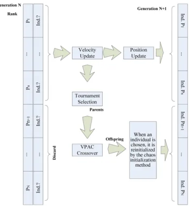
Here, the above chaos initialization method is used to initialize the whole swarm, and unlike BS, in the proposed CHA, the GA mutation process is not as the same as the traditional mutation method of changing the ‘0, 1’ sequence, but by chaos re-initialization. That is, when an individual is chosen to do the mutation, it is re-initialized by the chaos initialization method. For clarity, the flow of the proposed chaotic method is illustrated inFig. 1, wheren

=

(

N

· (

1

−

ϕ))

.

2.3. Opposition-based learning (OBL) scheme for CHA

After the opposition-based learning (OBL) scheme [14] was proposed, in a very short period of time, it has been applied to various research areas. The achieved empirical results confirm that the concept of opposition-based learning is general enough and can be utilized in a wide range of learning and optimization fields to make these algorithms faster. In this paper, as an acceleration strategy, the OBL is employed for the population initialization in the proposed CHA.

The definition of the opposite point is as follows:

LetP

(

x1

,

x2

, . . . ,

xD

)

be a point in aD-dimensional coordinate system withx1

,

x2

, . . . ,

xD

∈ ℜ

andxi

∈

(

ai

,

bi

)

. The

opposite pointP

˜

is completely defined by its coordinatesx

˜

1

, . . . ,

˜

xD, where:

˜

xi

=

ai

+

bi

−

xi

,

i

=

1

,

2

, . . . ,

D

.

(6)

(4)

Fig. 2. Pseudo code of the opposition-based chaos initialization inspired by Rahnamayan et al. [14].

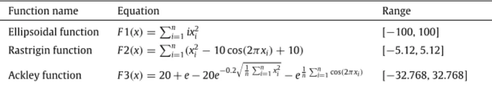
Table 1

Benchmark test functions.

Function name Equation Range

Ellipsoidal function F1(x)=n_i=1ix2i [−100, 100]

Rastrigin function F2(x)=n_i=1(xi2−10 cos(2πxi)+10) [−5.12, 5.12]

Ackley function F3(x)=20+e−20e−0.2  1 nni=1x2i−e1n n i=1cos(2πxi) _[−32.768, 32.768]

Assumef

(

x

)

is a fitness function which is used to measure the candidate’s fitness, then according to the definition of the opposite point,P

˜

=

(

x

˜

1

, . . . ,

˜

xD

)

is the opposite ofP

(

x1

,

x2

, . . . ,

xD

)

. Now, iff

(

P

˜

)

≥

f

(

P

)

, the point can be replaced with

˜

P; otherwise, continue withP. Hence, the pointPand its opposite point are evaluated simultaneously in order to continue with the fitter one.

In this paper, the opposition scheme [14] is combined with the proposed chaos initialization method. For clarity, the pseudo code of the novel Opposition-Based Chaos initialization method is shown inFig. 2, whereP0is the initial population,

OP0is the opposite of the initial population,Npis the population size,Pis the current population, andOPis the opposite of

the current population.

The Opposition-Based Chaos initialization method can be considered as a substitution for the aforementioned chaos initialization in CHA. Thus, the new Opposition-Based Chaotic initialization is adopted in the proposed CHA.

2.3.1. Test results

In order to test the effectiveness of the proposed CHA and the OBL scheme, three numeric optimization problems were chosen to compare the relative performance of the proposed CHA, CHA without the OBL scheme, BS, PSO and GA. These functions are standard benchmark test functions and are all minimization problems. Details are shown inTable 1.

Each function was run for 50 trials. Tests using 10 dimensions were allowed to run for 500 generations. Tests using 20 dimensions were allowed to run for 1000 generations. Finally tests using 30 dimensions were allowed to run for 1500 generations.

GA’s parameters in the setup were: population size 120, crossover ratio 0.75, mutation ratio 0.15, and maximum

generation 1500. PSO’s parameters in the setup were: swarm size 120, the inertia weight

ω

linearly decreasing from 0.9

to 0.2, the cognitive coefficientsc1

=

c2

=

2. For BS, tournament selection was used, with a tournament size of 3, to select

individuals as parents. Gaussian mutation was used, with mean 0.0 and variance reduced linearly for each generation from 1.0 to 0.1, the other parameters being the same as the PSO’s. For CHA and CHA without the OBL scheme, the parameters in the setup were the same as the Breeding Swarm. The testing results are shown inTable 2.

FromTable 2, although BS achieved better results in F1 and F3 with the dimension equal to 10, it can obviously be seen that the proposed CHA outperformed GA, PSO and BS in most runs when the dimension reached 20 and 30, through which the effectiveness of the novel chaotic approach has been fully illustrated. At the same time, the improvement made by the OBL scheme can obviously be seen through the comparison between test results of CHA and CHA without the OBL scheme. The OBL scheme does further enhance the searching power and effectiveness of the proposed method.

2.4. Species based CHA (SCHA)

Multimodal optimization is used to locate all the optima within the searching space, rather than one and only one optimum, and has been extensively studied by researchers. Many algorithms based on a large variety of different techniques

have been proposed in the literature. Recently, a species based particle swarm optimization (SPSO) method [23] was

introduced to solve multimodal problems. SPSO aims to identify multiple species within a population and determines the neighborhood best for each species. The multiple species are produced adaptively, in parallel, and used to optimize multiple optima. In this paper, Species based CHA (SCHA) is proposed by incorporating the notion of species into CHA.

(5)

Table 2

Benchmark test results.

Function Dims Gens GA (Mean and std. err.) PSO (Mean and std. err.) Breeding Swarm (Mean and std. err.)

CHA (without OBL) (Mean and std. err.)

CHA (Mean and std. err.)

F1

10 500 5.25E−03 4.59E−28 2.55E−28 5.29E−26 3.60E−26 (1.32E−03) 1.081E−28 (4.34E−28) (9.57E−26) (2.02E−26)

20 1000 2.06E−03 2.93E−28 3.00E−26 2.338E−33 1.942E−33 (1.02E−03) (5.30E−28) (7.43E−26) (3.291E−33) (2.85E−33)

30 1500 0.0735 2.495E−26 2.09E−23 4.75E−34 2.80E−34 (0.0231) (3.087E−26) (4.16E−23) (4.69E−34) (3.51E−34)

F2 10 500 2.329 5.632 3.2834 0 0 (1.561) (1.205) (1.2625) (0) (0) 20 1000 22.2022 12.013 9.2531 0.1990 0.099 (7.4051) (5.32) (2.2270) (0.3980) (0.2985) 30 1500 47.607 20.412 16.616 5.33E−16 2.53E−16 (12.302) (8.69) (2.920) (1.14E−15) (6.22E−16) F3

10 500 0.1820 4.175E−14 1.235E−14 4.317E−14 3.82E−14 (0.057) (1.628E−14) (2.186E−14) (2.168E−14) (1.88E−14)

20 1000 0.2261 6.48E−15 4.237E−14 6.217E−15 6.217E−15 (0.045) (2.13E−15) (2.621E−14) (0) (0)

30 1500 0.2502 2.087E−12 1.026E−12 6.68E−13 1.535E−14 (0.063) (0.674E−12) (1.283E−12) (9.44E−13) (3.21E−15)

2.4.1. Procedure of the SCHA

A species can be defined as a group of individuals sharing common attributes according to some similarity metric. This similarity metric could be based on the Euclidean distance for genotypes using a real coded representation. The smaller the Euclidean distance between two individuals, the more similar they are. The definition of species also depends on another parameter

γ

s, which denotes the radius measured in Euclidean distance from the center of a species to its boundary. The

center of a species, the so called species seed, is always the fittest individual in the species. All individuals that fall within the

γ

sdistance from the species seed are classified as the same species. The individuals start searching for the optimum of

a given objective function by moving through the search space from their initial positions. The manipulation of the whole population can be represented by Eqs.(7)and(8). Eq.(7)updates the individual velocity and Eq.(8)updates each individual’s position in the search space, where

ω

is the inertia weight,c1

,

c2are cognitive coefficients andr1

,

r2are two uniform random

numbers fromU

(

0

,

1

),

piis the personal best position andlbestiis the neighborhood best of individuali(each individual

hasDdimensions, andd

=

1

,

2

, . . . ,

D).

v

k+1 id

=

ωv

k id

+

c1r1

(

pkid

−

x k id

)

−

c2r2

(

lbestkid

−

x k id

)

(7) xk_id+1

=

x_idk

+

v

_idk+1

.

(8)

Once the species seeds have been identified from the population, one can then allocate each seed to be thelbestfor all the individuals in the same species at each iteration step. The algorithm for dividing the whole population into sub-species can be summarized in the following steps:

Step(1) Evaluate all individuals in the population.

Step(2) Sort all individuals in descending order of their fitness values (i.e., from the best fit to least fit ones).

Step(3) Determine the species seeds for the current population.

Step(4) Assign each species seed identified as the lbest to all individuals identified in the same species.

Step(5) Adjust the individual positions according to(7)and(8).

Step(6) Go back to Step(1),unless the termination condition is met.

Once the species seeds have been identified from the population, the whole population can then be divided into several sub-species. At each iteration step, all the individuals within each sub-species are updated by CHA. The whole procedure of SCHA is summarized inFig. 3.

2.4.2. Performance measurement

In order to test the ability of the proposed SCHA to locate the optima and the accuracy of the optima found, the peak ratio

and the average minimum distance to the real optima have been used as the performance metrics [29].

•

A peak is considered ‘found’ when an individual exists within 0.5 Euclidean distance to the peak in the last population. The peak ratio can be expressed in the following formula:

PeakRatio

=

Number of peaks found

(6)

Fig. 3. Pseudo code of the SCHA.

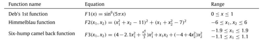
Table 3

Benchmark test functions.

Function name Equation Range

Deb’s 1st function F1(x)=sin6₍₅_π_x₎ ₀_≤_x_≤₁

Himmelblau function F2(x1,x2)=(x21+x2−11)2+(x1+x22−7)2 −6≤x1,x2≤6

Six-hump camel back function _F₃₍_x₁_,_x₂₎=(4−2.1x2 1+ x4 1 3)x 2 1+x1x2+(−4+4x22)x22 −1.9≤x1≤1.9 −1.1≤x1≤1.1

•

The average minimum distance to the real optima is determined using the following formula:

D

=

n



i=1 min indiv∈pop d

(

peak

,

indiv

)

n

wherenis the number of peaks,indivdenotes an individual andpopdenotes a population of individuals.

In the following section, all algorithms were run up to a maximum of 50 000 fitness function evaluations. The above performance metrics are obtained by taking the average and standard deviation of 30 runs.

To make it more clearly, thet-test (hypothesis testing) [30] is used to assess and compare the effectiveness and accuracy of different search algorithms. In a hypothesis test, we ask a question formulated in terms of a ‘‘TRUE or FALSE’’ statement called theNull Hypothesis, also denoted byH0. A null hypothesis,H0 will be correctly accepted with a significance (or

confidence) level

(

1

−

α)

and falsely rejected with a type I error probability

α

. Thet-test deals with the estimation of a true value from a sample and the establishing of confidence ranges within which the true value can said to lie with a certain probability

(

1

−

α)

. Hypothesis testing takes several steps to finally get at-value, which is then compared to thetcriticalvalue

(obtained fromt-distribution tables that are available in many basic statistics textbook). Ift

≤

tcritical, the null hypothesis is

then accepted with

(

1

−

α)

confidence level.

2.4.3. Test results

Three typical benchmark functions (Table 3) are introduced here to test the performance of the proposed SCHA. For

comparison, the notion of species is incorporated into the BS algorithm [3], named as Species based BS (SBS). Its procedure is similar to one in the proposed SCHA, just replacing the individuals’ updating rules by the BS method. The parameters in the setup, for both SBS and SCHA, are: swarm size 100, the inertia weight

ω

is linearly decreased from 0.9 to 0.2, the cognitive coefficientsc1

=

c2

=

2, tournament size 3, mutation ratio reducing linearly in each generation from 1.0 to 0.1.

As a comparison, the test results of Species Conserving Genetic Algorithm (SCGA) and Evolutionary Algorithm with Species-specific Explosion (EASE) [29] are also included.Table 4shows the experimental results, from which, one can observe that in most cases, promising results can be obtained by the proposed SCHA when compared with other methods. Although EASE achieved the best value in the minimum value ofDin F3, a minority of relatively poor results deteriorates the mean ofD. In general, SCHA is relatively more stable for locating optima.

To further compare the accuracy of SBS and SCHA,t-test is introduced. The null hypothesis has been defined as: SCHA

has higher accuracy than SBS. Defined

µ

as the average minimum distance to the real optima, thus:

H_α

:

µ

_SCHA

< µ

_SBS

(7)

Table 4

Experimental results of SCHA, SBS, EASE and SCGA.

Benchmark Measurement SCGA EASE SBS SCHA

F1

Mean ofD 1.32E−03 2.14E−10 3.26E−10 1.99E−10

StDev ofD 9.87E−04 6.71E−11 1.68E−10 1.52E−10 Min ofD 1.20E−04 1.22E−10 5.57E−11 1.15E−11

Median ofD 1.03E−03 2.01E−10 3.48E−10 1.58E−10

Mean of peak ratio 1.000 1.000 1.000 1.000

StDev of peak ratio 0.000 0.000 0.000 0.000

F2

Mean ofD 2.48E−01 1.12E−06 3.66E−06 3.58E−07

StDev ofD 1.27E−01 3.07E−06 1.01E−05 2.44E−07

Min ofD 5.72E−02 5.44E−07 1.10E−08 5.40E−09

Median ofD 2.11E−01 5.44E−07 5.16E−07 2.62E−07

F3

Mean ofD 1.10E−02 2.11E−06 4.03E−07 4.02E−07

StDev ofD 1.49E−02 9.36E−06 1.20E−09 1.10E−09

Min ofD 1.28E−04 3.91E−07 4.01E−07 4.01E−07 Median ofD 5.65E−03 4.02E−07 4.03E−07 4.02E−07

Table 5

Calculatedt-values for the accuracy hypotheses tests.

Functions Calculatedt-value,tcritical=2.5

Deb’s 1st function 2.6531 Himmelblau function 5.5814 Six-hump camel back function 2.5213

By taking

α

=

1%, andnSCHA

=

nSBS

=

10, this is a one sided test of significance of comparison of two means and

tcritical

=

2

.

5 [30]. Thet-statistic values, which were calculated for both the SCHA runs and SBS runs for the three benchmark

problems, are summarized inTable 5. It showst

>

tcriticalfor all test problems. These results lead to the rejection of the null

hypothesis and the acceptance of the alternative hypothesis with a confidence level of 99%. The interpretation of these results is that SCHA’s searching results are closer to the real optima than SBS’s, which also means that SCHA has a higher searching accuracy for all benchmark problems.

3. Application of the Species based CHA (SCHA) in circle detection

In this section, the proposed SCHA is applied to solve the circle detection problem. In this research, the three-edge-point circle representation method [27,31] has been adopted, which can reduce the search space by eliminating unfeasible circle locations.

3.1. Circle representation and fitness evaluation

Each circleCuses three edge points as individuals in the optimization algorithm. In this representation, edge points are stored as an index to their relative position in the edge arrayVof the image. This will encode an individual as the circle that passes through the three points

v

i

, v

jand

v

k.

Each circleCis represented by the three parametersx0

,

y0andr. With (x0

,

y0) being the (x

,

y) coordinates of the center

of the circle andrbeing its radius. One can compute the equation of the circle passing through the three edge points as:

(

x

−

x0

)

2

+

(

y

−

y0

)

2

=

r2 (9) with: x0

=



x2_j

+

y2_j

−

(

x2_i

+

y2_i

)

2

(

yj

−

yi

)

x2_k

+

y2_k

−

(

x2_i

+

y2_i

)

2

(

yk

−

yi

)



4

((

xj

−

xi

)(

yk

−

yi

)

−

(

xk

−

xi

)(

yj

−

yi

))

(10) y0

=



2

(

xj

−

xi

)

x2j

+

y 2 j

−

(

x 2 i

+

y 2 i

)

2

(

xk

−

xi

)

x2k

+

y 2 k

−

(

x 2 i

+

y 2 i

)



4

((

xj

−

xi

)(

yk

−

yi

)

−

(

xk

−

xi

)(

yj

−

yi

))

.

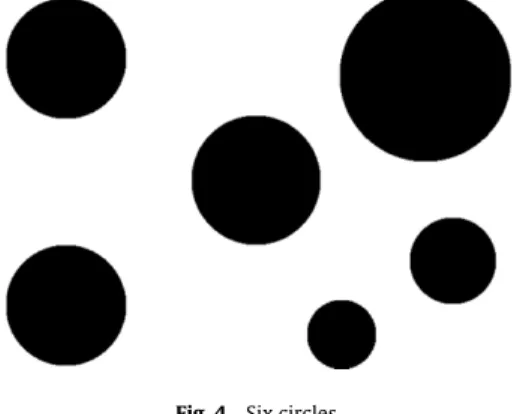
(11)

(8)

Fig. 4. Six circles.

The shape parameters (for the circle,

[

x0

,

y0

,

r

]

) can then be represented as a transformationTof the edge vector indexes

i

,

j

,

k.

[

x0

,

y0

,

r

] =

T

(

i

,

j

,

k

)

(12)

whereTis the transformation composed of the previous computations forx0

,

y0andr.

In order to compute the fitness value of a candidate circleC, the test set for the points is,S

= {

s1

,

s2

, . . . ,

sNs

}

withNs

the number of test points where the existence of an edge border is sought. The test point setSis generated by the uniform sampling of the shape boundary. In the case,Nstest points are generated around the circumference of the candidate circle.

Each pointsiis a 2D-point where its coordinates (xi

,

yi) are computed as follows:











xi

=

x0

+

r

·

cos 2

π

i Ns yi

=

y0

+

r

·

sin 2

π

i Ns

.

(13)

Fitness functionF

(

C

)

accumulates the number of expected edge points (i.e. the points in the setS) that actually are present in the edge image. That is:

F

(

C

)

=



_N s−1



i=0 E

(

xi

,

yi

)





Ns

.

(14)

WithE

(

xi

,

yi

)

being the evaluation of the edge features in the image coordinate (xi

,

yi) andNsbeing the number of pixels

in the perimeter of the circle corresponding to the circleCunder test. As the perimeter is a function of the radius, this serves as a normalization function with respect to the radius. That is,F

(

C

)

measures the completeness of the candidate circle and the objective is then to maximizeF

(

C

)

because a larger value implies a better circularity. Here, for clarity, a measurement of the completeness of the candidate circle is defined as the percentage of the points on the candidate circle that are actually present in the edge image and this measurement is indicated byCr:

Cr

=

Nt

/

Ns (15)

whereNt is the number of points on the candidate circle that are actually present in the edge image. So,Cr is a positive

number ranging from [0.0:1.0], and a larger value ofCrimplies a more complete circle.

3.2. Simulation results

To test the proposed SCHA-based method, five test images have been generated, with randomly located circles (Figs. 4–8). Results of interest are the center of the circle position and its diameter. The algorithms have been run 30 times for each test. The species radius

γ

sis defined as the distance between each two circles’ centers. For the three test images, the exact number

of circles and the distances between their centers are known, and the species radius

γ

swas normally set to a value smaller

than the distance between two closest circles.

For comparison, SBS and Species-based PSO (SPSO) [23] were used as solvers at the same time. All the trial tests were coded in MATLAB and executed on an Intel (R) 3.0 GHz CPU with a 2 GB RAM desktop computer. The parameters in the setup, for the SPSO were: swarm size 120, inertia weight

ω

decreasing linearly from 0.9 to 0.2, cognitive coefficientsc1

=

c2

=

2,

and maximum generation 5000. For both SBS and SCHA, the parameters were: tournament size 3, mutation ratio reducing linearly each generation from 1.0 to 0.1, and the other parameter settings were the same as for SPSO.

The simulation was conducted by running SCHA, SPSO and SBS 30 times. The minimal time, the mean time, the average value ofCrand the success rate are shown inTables 6–10. FromTables 6–9, it can be seen that for all of the three methods,

(9)

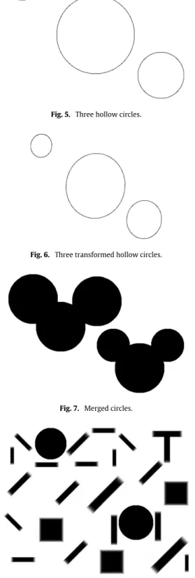
Fig. 5. Three hollow circles.

Fig. 6. Three transformed hollow circles.

Fig. 7. Merged circles.

Fig. 8. Two circles with other shapes.

SPSO, SBS and SCHA can achieve 100% success rate to locate all the circles, but the proposed SCHA-based method takes less time than the other two methods, and gives higherCrvalues in most cases. FromTable 10, the advantages of the proposed

(10)

Table 7

The simulation results on the test image of three hollow circles out of 30 runs.

Methods SPSO SBS SCHA

Time (mean and std. err) 0.34 s±0.101 0.29 s±0.149 0.28s±0.198

Time (minimum) 0.250 s 0.203 s 0.125s Cr(mean and std. err) 0.755±0.096 0.831±0.133 0.858±0.152

Success ratea_(%) ₁₀₀ ₁₀₀ ₁₀₀

a_{Success rate means how many times that all of the three circles can be}

successfully located during 30 runs.

Table 8

The simulation results on the test image of three transformed hollow circles out of 30 runs.

Success ratea_(%) ₁₀₀ ₁₀₀ ₁₀₀

a_{Success rate means how many times that all of the three transformed circles can be}

Table 9

The simulation results on the test image of merged circles out of 30 runs.

Success ratea_(%) ₁₀₀ ₁₀₀ ₁₀₀

a_{Success rate means how many times that all of the six merged circles can be}

Table 10

The simulation results on the test image of two circles with many other shapes out of 30 runs.

Success ratea_(%) _66.7 _76.7 ₁₀₀

a_{Success rate means how many times that both of the two circles can be successfully located}

during 30 runs.

can only achieve 66.7% and the SBS-based method can only achieve 76.7%. By using SCHA, the average error for localization is 0.15 pixels and maximum error (the worst case) is 0.72.

Figs. 9–13also show the plots of the average search time against the number of circles being detected in all the test images. Results for the SPSO-, the SBS- and the proposed SCHA-based methods are shown. For the first four test images, all the three methods can detect all the circles successfully but the proposed SCHA-based method is more efficient than the others. For the last test image, only the SCHA-based method has a 100% success rate. Neither the SPSO-based method nor the SBS-based method can detect both circles in all runs, which are represented by dashed lines inFig. 13.

From the simulation comparisons, it can be seen clearly that the proposed SCHA is much faster and more effective than both the SPSO- and the SBS-based methods. Thus, SCHA can be considered as a better means for solving multi-circle detection problems, and the detection results for the SCHA-based method can be seen inFigs. 14–18.

All the above test images have simple backgrounds, and that makes it easier for detecting circles as there are less edge points and at the same time, all the circles under test have very narrow edges. However, in reality, the circumstances will be

(11)

Fig. 9. Mean search time against the number of circles being detected in the test image of six circles.

Fig. 10. Mean search time against the number of circles being detected in the test image of three hollow circles.

Fig. 11. Mean search time against the number of circles being detected in the test image of three transformed hollow circles.

more complicated. The ‘circles’ may have wide edges and their shapes sometimes will not be that perfect. In order to detect them correctly, here, a method of ‘tolerant radius’ is proposed. This requires that when the fitness value of an individual reaches a threshold (marked asTh1), it is supposed that an imperfect circle is detected, and it gives the individual another two more chances to re-calculate its fitness value. This time, the method of ‘tolerant radius’ is used (Fig. 19), which allows the corresponding radius of the candidate circle (the black circumference inFig. 19) to have a tolerance of 5 pixels, either by moving inside (decreasing the radius to the blue dashed line circumference inFig. 19) or by moving outside (increasing the radius to the red dashed line circumference inFig. 19). If a real edge point falls in the area of the circular zones, either

(12)

Fig. 12. Mean search time against the number of circles being detected in the test image of merged circles.

Fig. 13. Mean search time against the number of circles being detected in the test image of two circles with other shapes.

Fig. 14. Detection result of the test image of six circles.

formed by the original candidate circle with the radius ofrand the circle with the radius ofr

−

5 pixels (the green zone in

Fig. 19) or is formed by the ones with a radius ofrandr

+

5 pixels (the pink zone inFig. 19), the corresponding point of the candidate circle is considered as effective. Hence, there will be another two fitness values re-calculated, and both will be no less than the original one. Then, another threshold (marked asTh2) is set for evaluation. If either of the two re-calculated fitness values can reachTh2, then the candidate circle under consideration is accepted.

With the help of the ‘tolerant radius’ method proposed above, more practical circle detection problems can be solved by the SCHA-based approach. For simulation tests, two hand drawn sketches and four natural photos are introduced.

(13)

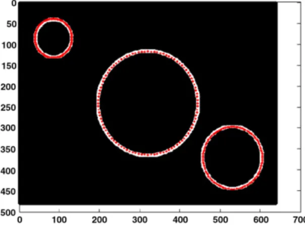
Fig. 15. Detection result of the test image of three hollow circles.

Fig. 16. Detection result of the test image of three transformed hollow circles.

Fig. 17. Detection result of test image of the merged circles.

The original images are shown inFigs. 20–25on the left, and the corresponding detection results are shown on the right. For each test image, the SCHA with the ‘tolerant radius’ method was run 30 times, and the corresponding running times are shown inTable 11.

The test results of the hand drawn sketches that are shown inFigs. 20and21can fully illustrate the effectiveness of the proposed ‘tolerant radius’ method. The blue circles in the detection results are the accepted candidate circles that have a ‘tolerant radius’, and the corresponding moving directions of the radii (either INSIDE or OUTSIDE) are also shown in the results. In the simulation tests using natural images, the ability of the proposed method in solving circle detection problems

(14)

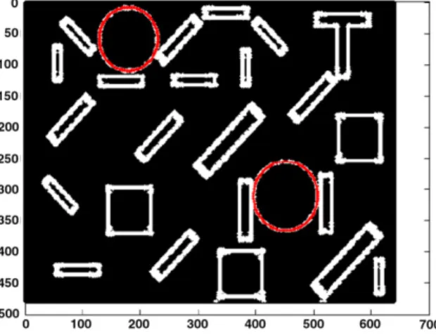
Fig. 18. Detection result of the test image of two circles with other shapes.

r+5

r–5 r

Fig. 19. Schematic of the candidate circle with ‘tolerant radius’.

Fig. 20. One-circle hand drawn sketch (on the left) and its detection result (on the right).

in the images with complicated backgrounds can clearly be revealed. Most of the circles in the natural images can directly be detected by the proposed SCHA-based method (the red circles in the detection results), and especially in the last test, the effectiveness of the ‘tolerant radius’ method is fully illustrated by detecting a big imperfect circle (the one highlighted by light-blue inFig. 25). In addition, the satisfactory success rate and running time of the proposed SCHA-based method are shown inTable 11. All these results fully prove the feasibility and effectiveness of the proposed method.

(15)

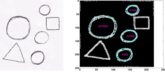
Fig. 21. Four-circle hand drawn sketch (on the left) and its detection result (on the right).

Fig. 22. Natural image no. 1 (on the left) and its detection result (on the right).

4. Conclusions and future work

In this paper, a novel Chaotic Hybrid Algorithm (CHA) is proposed, combining the strengths of particle swarm optimization with genetic algorithms. As an acceleration strategy, the opposition-based learning (OBL) scheme is employed

(16)

Table 11

The simulation results on the test images out of 30 runs. Test image One-circle hand

drawn sketch Four-circle hand drawn sketch Natural image no. 1 Natural image no. 2 Natural image no. 3 Natural image no. 4 Time (mean and std. err) 0.070 s±0.065 2.45 s±2.129 11.64 s±7.587 2.96 s±2.107 1.64 s±1.189 35.66 s±9.238 Time (minimum) 0.046 s 0.406 s 4.281 s 0.235 s 0.250 s 22.985 s

Success ratea_(%) ₁₀₀ ₁₀₀ ₁₀₀ ₁₀₀ ₁₀₀ ₁₀₀

a_{Success rate means how many times that all of the circles in the test images can be successfully located during 30 runs.}

for population initialization in the proposed CHA and in order to test the effectiveness of CHA, three numeric optimization problems were chosen to compare the relative performances of CHA with CHA without the OBL scheme, BS, PSO and GA. After proving the effectiveness of CHA through benchmarking, the notion of species was introduced into the novel algorithm to solve multimodal problems, leading to SCHA being proposed and subsequently applied for circle detection problems. In order to correctly detect circles in practical circumstances, the ‘tolerant radius’ concept has been proposed to enhance the circle detection process. After proving its effectiveness through simulations on five test images, SCHA has been combined with the proposed ‘tolerant radius’ method and successfully applied to solve single circle and multi-circle detection problems in hand drawn sketches and natural images.

As mentioned above, the advantages and effectiveness of this newly proposed optimization method has been fully illustrated through benchmarking and applications in the circle detection. In the future work, we would like to expand its application areas to function optimization, pattern recognition, optimization design, fuzzy logic control, scheduling and many others, in which PSO and GA have been wildly applied. We believe promising results can be expected by incorporating this novel chaotic hybrid algorithm. Also, it is worthwhile to explore the possibility of improving or integrating existing evolutionary and meta-heuristics algorithms.

Acknowledgments

Our gratitude is extended to the Research Committee and the Department of Industrial and Systems Engineering of the Hong Kong Polytechnic University for support in this project (G-U726). This work was also supported in part by the Application Base and Frontier Technology Research Project of Tianjin, China under 08JCZDJC21900.

(17)

References

[1] P. Angeline, Evolutionary optimization versus particle swarm optimization: philosophy and performance differences, in: Evolutionary Programming, in: LNCS, vol. 1447, 1998, pp. 601–610.

[2] R. Eberhart, Y. Shi, Comparison between genetic algorithms and particle swarm optimization, in: Evolutionary Programming, in: LNCS, vol. 1447, 1998, pp. 611–616.

[3] M. Settles, T. Soule, Breeding swarms: a GA/PSO hybrid, in: Proceedings of the Genetic and Evolutionary Computation Conference, GECCO, Washington, DC, USA, 2005.

[4] K.W. Wong, S.H. Kwok, W.S. Law, A fast image encryption scheme based on chaotic standard map, Phys. Lett. A 372 (2008) 2645–2652.

[5] Z. Lu, L.S. Shieh, G.R. Chen, On robust control of uncertain chaotic systems: a sliding mode synthesis via chaotic optimization, Chaos Solitons Fractals 18 (2003) 819–827.

[6] H.R. Tizhoosh, Opposition-based learning: a new scheme for machine intelligence, in: International Conference on Computational Intelligence for Modelling Control and Automation, CIMCA, Vienna, Austria, 2005.

[7] H.R. Tizhoosh, Reinforcement learning based on actions and opposite actions, in: International Conference on Artificial Intelligence and Machine Learning, AIML, Cairo, Egypt, 2005.

[8] H.R. Tizhoosh, Opposition-based reinforcement learning, J. Adv. Comput. Intell. Intell. Inform. 10 (4) (2006) 578–585.

[9] M. Shokri, H.R. Tizhoosh, M. Kamel, Opposition-basedQ(l) algorithm, in: 2006 IEEE World Congress on Computational Intelligence, IJCNN, Vancouver, BC, Canada, 2006.

[10] H.R. Tizhoosh, M. Shokri, M.S. Kamel, Opposition-basedQ(lambda) with non-Markovian update, in: IEEE Symposium on Foundations of Computational Intelligence, Honolulu, Hawaii, USA, 2007.

[11] H.R. Tizhoosh, M. Mahootchi, K. Ponnambalam, Opposition-based reinforcement learning in the management of water resources, in: IEEE Symposium on Foundations of Computational Intelligence, Honolulu, Hawaii, USA, 2007.

[12] F. Sahba, H.R. Tizhoosh, M.M.A. Salama, Application of opposition based reinforcement learning in image segmentation, IEEE Symposium on Foundations of Computational Intelligence, Honolulu, Hawaii, USA, 2007.

[13] S. Rahnamayan, H.R. Tizhoosh, M.M.A. Salama, A novel population initialization method for accelerating evolutionary algorithms, Comput. Math. Appl. 53 (10) (2007) 1605–1614. (Elsevier).

[14] S. Rahnamayan, H.R. Tizhoosh, M.M.A. Salama, Opposition-based differential evolution, IEEE Trans. Evol. Comput. 12 (1) (2008) 64–79.

[15] S. Rahnamayan, H.R. Tizhoosh, M.M.A. Salama, Opposition-based differential evolution (ODE) with variable jumping rate, in: IEEE Symposium on Foundations of Computational Intelligence, Honolulu, Hawaii, USA, 2007.

[16] M. Ventresca, H.R. Tizhoosh, Improving the convergence of backpropagation by opposite transfer functions, in: 2006 IEEE World Congress on Computational Intelligence, IJCNN, Vancouver, BC, Canada, 2006.

[17] M. Ventresca, H. Tizhoosh, Opposite transfer functions and backpropagation through time, in: IEEE Symposium on Foundations of Computational Intelligence, Honolulu, Hawaii, USA, 2007.

[18] M. Ventresca, H. Tizhoosh, Simulated annealing with opposite neighbors, in: IEEE Symposium on Foundations of Computational Intelligence, Honolulu, Hawaii, USA, 2007.

[19] H.R. Tizhoosh, A.R. Malisia, Applying opposition-based ideas to the ant colony system, in: IEEE Symposium on Foundations of Computational Intelligence, Honolulu, Hawaii, USA, 2007.

[20] F. Khalvati, H.R. Tizhoosh, M.D. Aagaard, Opposition-based window memorization for morphological algorithms, in: IEEE Symposium on Foundations of Computational Intelligence, Honolulu, Hawaii, USA, 2007.

[21] Y.G. Petalas, C.G. Antonopoulos, T.C. Bountis, M.N. Vrahatis, Detecting resonances in conservative maps using evolutionary algorithms, Phys. Lett. A 373 (2009) 334–341.

[22] D.E. Goldberg, J. Richardson, Genetic algorithms with sharing for multimodal function optimization, in: Proc. of the Second International Conference on Genetic Algorithms, ICGA, New Jersey, 1987.

[23] D. Parrott, X. Li, Locating and tracking multiple dynamic optima by a particle swarm model using speciation, IEEE Trans. Evol. Comput. 10 (4) (2006) 440–457.

[24] W. Lam, S. Yuen, Efficient techniques for circle detection using hypothesis filtering and Hough transform, IEEE Proc. Vis. Image Signal Process. 143 (5) (1996) 292–300.

[25] T. Mainzer, Genetic algorithm for shape detection, Technical Report DCSE/TR-2002-06, University of West Bohemia in Pilsen, Pilsen, Czech Republic, 2002.

[26] P.L. Rosin, H.O. Nyongesa, Combining evolutionary, connectionist, and fuzzy classification algorithms for shape analysis, in: Cagnoni, S. et al. (Eds.), Proc. EvoIASP, Real-World Applications of Evolutionary Computing, 2000.

[27] A.R. Victor, H.G. Carlos, P.G. Arturo, E.S. Raul, Circle detection on images using genetic algorithms, Pattern Recognit. Lett. 27 (6) (2006) 652–657. [28] H. Zhang, J.H. Shen, T.N. Zhang, Y. Li, An improved chaotic particle swarm optimization and its application in investment, in: Proceedings of the

International Symposium on Computational Intelligence and Design, ISCID, Wuhan, China, 2008.

[29] K.C. Wong, K.S. Leung, M.H. Wong, An evolutionary algorithm with species-specific explosion for multimodal optimization, in: Proc. of the 11th Annual Conference on Genetic and Evolutionary Computation, GECCO, ACM, New York, 2009.

[30] R. Hassan, B. Cohanim, O. de Weck, G. Venter, A comparison of particle swarm optimization and the genetic algorithm, in: 1st AIAA Multidisciplinary Design Optimization Specialist Conference, No. AIAA-2005-1897, Austin, TX, 2005.

[31] C.H. Wu, N. Dong, W.H. Ip, C.Y. Chen, K.L. Yung, Z.Q. Chen, Chaotic hybrid algorithm and its application in circle detection, Lecture Notes in Comput. Sci. 6024 (2010) 302–311.