Deliverable 5 Proposal for Harmonised Guidelines

(1)

Contract No. FP6-2002-SSP-1/502481

HEATCO

Developing

H

armonised

E

uropean

A

pproaches for

T

ransport

Co

sting and Project Assessment

Specific Support Action

PRIORITY SSP 3.2: The development of tools, indicators and operational parameters for assessing sustainable transport and energy systems performance (eco-nomic, environmental and social)

Deliverable 5

Proposal for Harmonised Guidelines

Due date of deliverable: 15 December 2005

Actual submission date: February 2006

Start date of project: 29 February 2004

Duration: 27 months

Lead contractor for this deliverable: IER, Germany

(2)

ii

HEATCO Deliverable 5

Proposal for Harmonised Guidelines

Peter Bickel Rainer Friedrich Arnaud Burgess Patrizia Fagiani Alistair Hunt Gerard De Jong James Laird Christoph Lieb Gunnar Lindberg Peter Mackie Stale Navrud Thomas Odgaard Andrea Ricci Jeremy Shires Lori Tavasszy

(3)

Contents

0 Summary S1

0.1 Introduction S1

0.2 General issues S2

0.3 Value of time and congestion S4

0.3.1 Valuation Methodology S4

0.3.2 VTTS values S4

0.3.3 Treatment of Congestion S5

0.3.4 Treatment of Uncertainty in VTTS values S7

0.3.5 Implementation of VTTS Guidelines S7

0.4 Value of changes in accident risks S14

0.5 Environmental costs S17

0.5.1 Air pollution S17

0.5.2 Noise S22

0.5.3 Global warming S25

0.5.4 Other effects S26

0.6 Costs and indirect costs of infrastructure investment S26 0.6.1 Capital costs of the infrastructure investment S27

0.6.2 Residual value S27

0.6.3 Optimism-bias S28

0.6.4 "Costs of maintenance, operation and administration" and "Changes in

infrastructure costs on existing network" S29

0.7 Vehicle operating costs S32

1 Introduction 1

1.1 Transport appraisal 1

1.2 Transport appraisal within the policy process 3

1.3 The HEATCO guidelines and other supra-national guidelines at a EU level 3

1.4 The structure of these guidelines 7

2 Transport Cost Benefit Analysis 9

2.1 Overview 9

2.2 Scope of CBA 11

2.3 Definition of alternatives 11

2.4 Transport User Benefits 12

2.5 Impacts on Transport Providers and Government 13

2.5.1 Producer surplus 13

2.5.2 Investment costs 15

(4)

Contents HEATCO D5

iv

2.5.4 Taxation and government revenue effects 16

2.6 Safety benefits 17

2.7 Impacts on the Environment 17

2.8 Cost Benefit Analysis Parameters 18

2.9 Risk and Uncertainty 18

2.10 Reporting the Cost Benefit Analysis 19

3 General Issues 21

3.1 Non-market valuation techniques 21

3.1.1 Definitions 21

3.1.2 Purpose/role in project appraisal 22

3.1.3 Existing practice at EC and national levels 22

3.1.4 Best practice 22

3.1.5 Recommendations 24

3.2 Value Transfer 25

3.3 Treatment of non-monetised impacts 27

3.4 Discounting and intra-generational equity issues 29

3.5 The project appraisal evaluation period 38

3.5.3 Existing practice at EC and nation al levels 38

3.6 Decision criteria 39

(5)

HEATCO D5 Contents

3.7 Treatment of future risk and uncertainty 45

3.8 The Marginal Costs of Public Funds 47

3.9 Producer Surplus of Transport Providers 49

3.9.2 Existing and Best practice 49

3.10 Treatment of indirect socio-economic effects in European guidelines for transport appraisal 50

3.11 Recommended Accounting procedures 52

3.12 Up-dating of values 52

4 Value of Time and Congestion 53

4.1 Purpose/role in project appraisal 53

4.2 Definition 53

4.3 Valuation Methodology 53

4.4 VTTS values 55

4.4.1 Disaggregation 55

4.4.2 Variation of Passenger VTTS with income 57

4.4.3 Variation of Passenger VTTS with journey length 59 4.4.4 Variation of Passenger VTTS by journey purpose 59 4.4.5 Variation of Passenger VTTS by mode, walking, waiting, interchange and

(6)

Contents HEATCO D5

vi

4.4.6 Variation of Commercial Goods Traffic VTTS 61

4.4.7 Size and sign of time savings 62

4.4.8 Treatment of values of travel time savings over time 63

4.4.9 Uncertainty in the VTTS value 64

4.5 Treatment of congestion 65

4.5.1 Reliability 66

4.5.2 Public transport overcrowding 68

4.5.3 Quality of travel experience 69

4.6 Implementation of VTTS Guidelines 70

4.6.1 Deriving VTTS for use in an appraisal 70

4.6.2 VTTS data requirements 78

4.6.3 VTTS in modelling and appraisal 80

4.6.4 Reporting and equity 80

5 Value of Changes in Accident Risks 81

5.2 General Approach 81

5.2.1 Accident impacts considered 82

5.2.2 Estimating accident risks 82

5.2.3 Valuing accident costs 84

5.2.4 Recommended values 87

5.2.5 Treatment of values over time 89

5.2.6 Calculation procedure 90

6 Environmental Costs 91

6.2 General Valuation Methodology 91

6.3 Air pollution 94

6.3.1 Derivation of impact and cost factors per unit pollutant emitted 95

6.4 Noise 103

6.4.1 Noise impact assessment 104

6.4.2 Monetary Valuation 105

6.5 Global warming 115

6.5.1 General approach 115

6.5.2 Monetary values 116

(7)

HEATCO D5 Contents

6.6 Other effects 118

7 Costs and Indirect Costs of Infrastructure Investment 119

7.1 Introduction 119

7.2 Whole life costing 119

7.3 Capital costs of the infrastructure investment 120

7.4 Residual value 123 7.4.1 Justification/motivation 123 7.4.2 Recommendation 123 7.5 Optimism-bias 125 7.5.1 Justification/motivation 125 7.5.2 Recommendation 126

7.6 "Costs of maintenance, operation and administration" and "Changes in

infrastructure costs on existing network" 129

7.6.1 Justification/motivation 130

7.6.2 Recommendation 130

8 Vehicle Operating Costs 135

8.2 Definition 135

8.3 Valuation Methodology 136

8.3.1 Core Issues 136

8.3.2 Road vehicle operating costs 137

8.3.3 Train operating costs 137

8.3.4 Ship and aircraft operating costs 138

8.4 Implementation of vehicle operating cost guidelines 138 8.4.1 Deriving vehicle operating costs for use in an appraisal 138

8.4.2 Vehicle operating cost data requirements 139

9 References 141

(8)

viii

List of Tables

Table 0.1 Recommended valuation methodologies. 4 Table 0.2 Reliability ratios (Source: Hamer et al. (2005), Kouwenhoven et al. (2005a)). 6 Table 0.3 Estimated VTTS values – work (business) passenger trips (€2002 per passenger per hour,

factor prices) 9

Table 0.4 Estimated VTTS values – non-work passenger trips (€2002 per passenger per hour, factor

prices) 10

Table 0.5 Estimated VTTS values – freight trips (€2002 per freight tonne per hour, factor prices) 11 Table 0.6 Estimated VTTS values – work (business) passenger trips (€2002 PPP per passenger per

hour, factor prices) 12

Table 0.7 Estimated VTTS values – non-work passenger trips (€2002 PPP per passenger per hour,

factor prices) 13

Table 0.8 Estimated VTTS values – freight trips (€2002 PPP per freight tonne per hour, factor prices) 14 Table 0.9 Recommendation for European average correction factors for unreported road accidents.

15 Table 0.10 Estimated values for casualties avoided. 16 Table 0.11 Cost factors for road transport emissions* per tonne of pollutant emitted in €2002 (factor

prices). 19 Table 0.12 Cost factors for road transport emissions* per tonne of pollutant emitted in €2002 PPP

(factor prices). 20

Table 0.13 Impact factors for road transport emissions* (lost life expectancy in years of life lost per

1000 tonnes of pollutant emitted). 21

Table 0.14 Cost factors for noise exposure for Finland (€2002, factor costs, per year per person exposed; to derive €2002 PPP the values below are divided by the Finish PPP adjustment factor of 1.12). For values for all countries see main text. 23 Table 0.15 Impact indicator for noise exposure: percentage of adult persons highly annoyed per

person (all ages) exposed – based on functions given in European Commission (2002),

assuming 80% of population are adults. 24

Table 0.16 Shadow prices based on Watkiss et al. (2005b), converted from ₤2000/t C to €2002 (factor prices) per tonne of CO2 equivalent emitted – no PPP adjustment necessary as values are

not country specific. 26

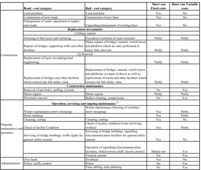
Table 0.17 Lifetimes by mode and group of components (road and rail). 28 Table 0.18 Applicable capital expenditure uplift (average cost escalation) 29 Table 0.19 Classification of cost categories into short run fixed costs and short run variable costs -

Road and rail. 30

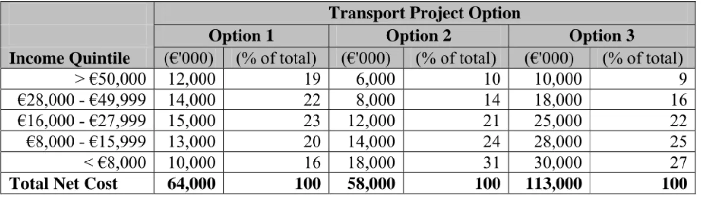
Table 0.20 Possible allocation factors for the allocation of variable costs to cost drivers. 31 Table 1.1 DG Regional Policy Guidelines, TINA, RAILPAG, HEATCO: a comparative overview. 5 Table 3.1 Example Distributional Matrix for a Transport Project Appraisal. 32 Table 3.2 Net present value (NPV) versus benefit cost ratio (BCR) 41 Table 3.3 The labelling of noise as costs or benefits determines the ranking list 41 Table 4.1 Recommended valuation methodologies. 54 Table 4.2 Recommended level of disaggregation for travel time savings. 57

Table 4.3 Reliability ratios. 67

Table 4.4 Approximating the underlying willingness-to-pay of traffic on the TEN-T. 71 Table 4.5 Recommended source for deriving passenger VTTS (based on 2004 survey of EU

member states appraisal methodology). 72

Table 4.6 Estimated VTTS values – work (business) passenger trips (€2002 per passenger per hour,

(9)

HEATCO D5 List of Tables

Table 4.7 Estimated VTTS values – non-work passenger trips (€2002 per passenger per hour, factor

prices) 74

Table 4.8 Estimated VTTS values – freight trips (€2002 per freight tonne per hour, factor prices) 75 Table 4.9 Estimated VTTS values – work (business) passenger trips (€2002 PPP per passenger per

hour, factor prices) 76

Table 4.10 Estimated VTTS values – non-work passenger trips (€2002 PPP per passenger per hour,

factor prices) 77

Table 4.11 Estimated VTTS values – freight trips (€2002 PPP per freight tonne per hour, factor prices) 78 Table 4.12 Use of local data or benefit transfer procedures. 79 Table 5.1 Recommendation for European average correction factors for unreported road accidents.

83 Table 5.2 Estimated values for casualties avoided (€2002, factor prices). 88 Table 5.3 Estimated values for casualties avoided (€2002 PPP, factor prices). 89 Table 6.1 Health and environmental effects for which exposure-response functions are established

(source: European Commission, 2005). 95

Table 6.2 Cost factors for road transport emissions* per tonne of pollutant emitted in €2002 (factor

prices). 97 Table 6.3 Cost factors for road transport emissions* per tonne of pollutant emitted in €2002 PPS

(factor prices). 98

Table 6.4 Cost factors for electricity production emissions* per ton of pollutant emitted in €2002

(factor prices). 99

Table 6.5 Cost factors for electricity production emissions* per ton of pollutant emitted in €2002 PPS

(factor prices). 100

Table 6.6 Impact factors for road transport emissions* (lost life expectancy in years of life lost per

1000 tonnes of pollutant emitted). 101

Table 6.7 Impact factors for electricity production emissions* (lost life expectancy in years of life lost per 1000 tonnes of pollutant emitted). 102 Table 6.8 Categorisation of effects and related impact categories (source: De Kluizenaar et al.,

2001). 104 Table 6.9 Cost factors (Central values) for noise exposure (€2002, factor costs, per year per person

exposed). High values and results for the new approach see Annex E. 106 Table 6.10 Cost factors (Central values) for noise exposure (€2002 PPP, factor costs, per year per

person exposed). High values and results for the new approach see Annex E. 110 Table 6.11 Impact indicator for noise exposure: percentage of adult persons highly annoyed per

person (all ages) exposed – based on functions in European Commission (2002),

assuming 80% of population are adults. 114

Table 6.12 Shadow prices based on Watkiss et al. (2005b), converted from ₤2000/t C to €2002 (factor prices) per tonne of CO2 equivalent emitted. 117 Table 7.1 Lifetimes in years by mode and group of components (road and rail). 124 Table 7.2 Example 1: "No re-investments" (million €) 125 Table 7.3 Example 2: "Re-investments" (million €) 125 Table 7.4 Ideas to reduce uncertainty/cures to optimism-bias. 126 Table 7.5 Applicable capital expenditure uplift (average cost escalation) 128 Table 7.6 Classification of cost categories into short run fixed costs and short run variable costs -

road and rail. 131

Table 7.7 Possible allocation factors for the allocation of variable costs to cost drivers. 132 Table 8.1 Approximating the underlying resource costs for operating vehicles on the TEN-T. 140

(10)

x

List of Figures

Figure 6.1 The Impact Pathway Approach for the quantification of environmental costs. 92

Figure 7.1 Whole life costing approach 120

Figure 7.2 Definition of optimism-bias uplifts within a certain class. Source: Based on the British Department for Transport (2004b, page 11) 128

Abbreviations

ATOC Association of Train Operating Companies BCR Benefit-Cost Ratio

CBA Cost Benefit Assessment

EIA Environmental Impact Assessment ESA Equivalent standard axles

FYRR First Year Rate of Return GWP Global Warming Potential HGV Heavy Goods Vehicle

IFI International financing institution IPA Impact Pathway Approach

IRR Internal Rate of Return IVT In Vehicle Time LGV Light Goods Vehicle

MS Member States

NPV Net Present Value

PDFH Passenger Demand Forecasting Handbook (UK) PPP Purchasing Power Parity

PVB Present Value of Benefits PVC Present Value of Costs

RNPSS Ratio of NPV and Public Sector Support VOC Vehicle Operating Costs

VSL Value of a Statistical Life VTTS Value of Travel Time Savings WTP Willingness to Pay YOLL Years of Life Lost

(11)

0 Summary

0.1 Introduction

The objective of this document is to propose harmonised guidelines for project assessment for trans-national projects in Europe. This includes the provision of a consistent framework for monetary valuation based on the principles of welfare economics, contributing in the long run to consistency with transport costing. These guidelines have been developed within the EC funded research project HEATCO, based on latest research results on the different aspects of transport project appraisal and on an analysis of existing practice in the EU countries and Switzerland.

The review of existing practice documented in Odgaard et al. (2005) and further analysed in Bickel et al. (2005a) has shown considerable variation. In the context of selecting and finan-cially supporting TEN-T projects, the need for consistent appraisal methodology arises. Thus, a consistent methodological framework for project appraisal has been developed and is de-scribed here. Apart from being used for TEN-T projects, it might also be used for other trans-national projects to ensure consistency across borders and the application of the state of the art methods. It is not the intention of HEATCO’s proposal for harmonised guidelines to stipu-late methods and values for national projects, however in the long run these guidelines might help to achieve a more harmonised approach also for national appraisal methods.

This summary gives an overview of the recommendations for harmonised guidelines for infrastructure project appraisal covering the following elements:

• General issues (incl. market valuation techniques, benefit transfer, treatment of non-monetised impacts, discounting and intra-generational equity issues, decision criteria, the project appraisal evaluation period, treatment of future risk and uncertainty, the marginal costs of public funds, producer surplus of transport providers, the treatment of indirect socio-economic effects),

• Value of time and congestion (incl. business passenger traffic, non-work passenger traffic, commercial goods traffic time savings and treatment of congestion, unexpected delays and reliability),

• Value of changes in accident risks (incl. accident impacts considered, estimating accident risks, valuing accident costs),

• Environmental costs (incl. air pollution, noise, global warming),

• Costs and indirect impacts of infrastructure investments (incl. capital costs for project implementation, costs for maintenance, operation and administration, changes in infra-structure costs on existing networks, optimism bias, residual value).

Country-specific fall-back values are suggested for application in cases where no state-of-the-art national values are available for valuation of

• time and congestion,

• accident casualties,

(12)

S2

Summary HEATCO D5

0.2 General issues

When carrying out a Cost-Benefit Analysis (CBA), we recommend the following 15 general principles:

1. Appraisal as a comparative tool. To estimate the costs and benefits of a project, one has to compare costs and benefits between two scenarios: the ‘Do-Something’ scenario, where the project under assessment is realised, and a ‘Do-Minimum’ scenario, which needs to be a realistic base case describing the future development. If there are several project alterna-tives, one has to create a scenario for each alternative and compare them with the ’Do-minimum case’.

2. Decision criteria. We recommend the use of NPV (net present value) to determine, whether a project is beneficial or not. In addition, depending on the decision-making con-text respectively the question to be addressed, BCR (benefit cost ratio) and RNPSS (ratio of NPV and public sector support) decision rules could be used.

3. The project appraisal evaluation period. We recommend the use of a 40 year appraisal period, with residual effects being included, as a default evaluation period. Projects with a shorter lifetime should, however, use their actual length. For the comparison of potential future projects, a common final year should be determined by adding 40 years to the open-ing year of the last project.

4. Treatment of future risk and uncertainty. For the assessment of (non-probabilistic) uncer-tainty, we consider a sensitivity analysis or scenario technique as appropriate. If resources and data are available for probabilistic analysis, Monte Carlo simulation analysis can be undertaken.

5. Discounting. It is recommended to adopt the risk premium-free rate or weighted average of the rates currently used in national transport project appraisals in the countries in which the TEN-T project is to be located. The rates should be weighted with the proportion of total project finance contributed by the country concerned. In lower-bound sensitivity analyses, in order to reflect current estimates of the social time preference rate, a common discount rate of 3% should be utilised. For damage occurring beyond the 40 year appraisal period (intergenerational impacts), e.g. for climate change impacts, a declining discount rate system is recommended.

6. Intra-generational equity issues. We recommend, at minimum, that a “winners and losers” table should be developed, and presented alongside the results of the monetised CBA. Distributional matrices for alternative projects might be created and compared amongst each other. Additionally stakeholder analyses should be undertaken as well. It is recom-mended to use local values to assess unit benefit and cost measures.

7. Non-market valuation techniques. If impacts in transport project appraisals cannot be expressed in market prices, but are potentially significant in the overall appraisal, we rec-ommend that – in the absence of robust transfer values – non-market techniques to esti-mate monetary values should be considered. We recommend that the choice of technique used to value individual impacts should be dictated by the type of impact and the nature of the project. However, Willingness to Pay (WTP) measures is preferable to cost-based measures. Values should be validated against existing European estimates.

8. Value Transfer.Value transfer means the use of economic impact estimates from previous studies to value similar impacts in the present appraisal context. Value transfers can be used when insufficient resources for new primary studies are available. The decision as to

(13)

HEATCO D5 Summary

whether to use unit transfers with income adjustments, value function transfer and/or meta-analyses will depend on the availability of existing values and experience to date with value transfers related to the impact in question.

9. Treatment of non-monetised impacts. We recommend, at a minimum, that if impacts cannot be expressed in monetary terms, they should be presented in qualitative or quanti-tative terms in addition to evidence on monetised impacts. If only a small number of non-monetised impacts can be assessed, sensitivity analysis may be used to indicate their po-tential importance. Alternatively, non-monetised impacts may also be included directly in the decision-making process by explicitly eliciting decision maker’s weights for them vis-à-vis monetised impacts.

10.Treatment of indirect socio-economic effects. We recommend that if indirect effects are likely to be significant, an economic model, preferably a Spatially Computable General Equilibrium (SCGE) model, should be used. Qualitative assessment is recommended, if indirect effects cannot be modelled due to limited resources (high costs for the use of ad-vanced modelling), insufficient availability of data, or lack of appropriate quantitative models or unreliable results.

11.Marginal Cost of Public Funds. Our recommendation is to assume a marginal cost of public funds of 1, i.e. not to use any additional cost (shadow price) for public funds. In-stead, a cut-off value for the RNPSS of 1.5 should be used when relevant.

12.Producer Surplus of Transport Providers. We recommend to estimate (changes in) the producer surplus generated by changed traffic volumes or by the introduction and adjust-ment of transport pricing regimes.

13.Accounting procedures. a) Factor costs should be the adopted unit of account. This re-quires measures expressed in market prices - which include indirect taxes and subsidies – to be converted to factor costs. b) We recommend to convert all monetary values into € with a price level for a fixed year. In this report, monetary values are given as €2002, i.e.

with 2002 as base year. However, the monetary values should be adjusted with the Pur-chasing Power Parity (PPP) as explained in Annex B, which also contains a table with PPP adjustment factors. However, these factors are only available for past years, whilst future PPP factors are likely to change as the economic growth rates differ amongst coun-tries. As we assume, that income and prices grow faster in Member States with currently low income, PPP factors will tend to converge closer to 1 in the future. Therefore, we recommend that two calculations are made – one with and one without PPP adjustment – assuming that the true value will lie between the two results. c) Monetary values, i.e. pref-erences, for non-market goods like reduced risk of getting ill or reduced damage to the environment will increase with increasing income; thus we recommend increasing mone-tary values based on GDP growth – a table with possible country-specific GDP growth is given in Annex B.

14.Up-dating of values. The unit values supplied in this report represent the state-of-the-art for the individual impacts addressed. Nevertheless, all values will be subject to change as new empirical evidence becomes available and methodological developments take place. As a consequence, we recommend that values are reviewed and up-dated on a regular ba-sis e.g. after three years at maximum.

15.Presentation of results. As far as possible, impacts should be expressed in both physical and monetary terms. The results of the sensitivity analysis and the non-monetised impacts should be reported together with the central monetised results.

(14)

S4

Summary HEATCO D5

0.3 Value of time and congestion

0.3.1 Valuation Methodology

The underlying principle in the VTTS (value of travel time savings) guidelines is that local values should be used wherever possible, provided that they have been developed using an appropriate methodology. If no such local values exist then ‘default’ or ‘fallback’ values derived from international meta-analyses of value of time studies should be used. These fallback values are set out in Table 0.3, Table 0.4 and Table 0.5.

Economic theory suggests that different methods of valuation for VTTS should be used for passenger trips during work, that is to say on employer’s business, for passenger-non-work trips, that is for commuting, shopping and leisure purposes, and for commercial goods traffic. As set out in Table 0.1 for each of these purposes we recommend a minimum acceptable methodology for the valuation of time savings. The cost saving approach for employer’s business and commercial traffic is based on a theoretical argument regarding the marginal productivity of labour. Such an approach assumes no utility impact on the worker and that all travel time savings can be transferred to productive output. The more sophisticated Hensher approach (Hensher, 1977) allows for the fact that not all travel time is unproductive and not all savings are transferred to extra work. Willingness-to-pay surveys are based on either the revealed or stated preferences of individuals.

Table 0.1 Recommended valuation methodologies.

Trip Purpose Minimum approach1 More sophisticated approach

Passenger – work Cost saving Hensher approach

Passenger – non-work Willingness-to-pay

Commercial Goods traffic Cost saving Willingness-to-pay

1_{In the absence of sufficient resources to survey VTTS using the minimum approach the}

mathematical relationships derived from the HEATCO VTTS meta-analysis should be used.

0.3.2 VTTS values Disaggregation

At a minimum, VTTS values should be disaggregated between work, passenger-non-work and commercial goods traffic. This is recommended because different valuation methods are used to calculate VTTS values for each of these purposes. Furthermore, due to the very different functions served by the various transport modes when transporting freight, commercial goods traffic should be disaggregated by mode at a minimum. For more sophisti-cated appraisals passenger VTTS could be disaggregated by mode and/or distance. A more data intensive and refined level of disaggregation would be to disaggregate by trip purpose, income, journey length and modal comfort. Disaggregation by income is strongly recom-mended for major infrastructure projects or projects that involve some form of user charging (tolled motorways, high speed rail, etc.). In such cases, consistency between values used in demand modelling and appraisal is required.

(15)

Walk, wait and interchange

In the absence of local data on travel time savings for walking, waiting and interchange, in-vehicle time should be weighted in order to reflect the additional willingness-to-pay for time savings. In-vehicle time should be weighted by 2 for walking time and 2.5 for waiting and interchange (or transfer) time.

Average waiting times for public transport services will vary systematically with the headway of the services. At high frequencies passengers arrive at random and the average idle time is half the headway. It is recommended that the modelling exercise explicitly models average waiting periods associated with the different service frequencies, and this time should be included in the appraisal weighted with a factor of 2.5. At lower frequencies arrival rates are not at random and average waiting times do not fully capture all the costs or benefits of a change in frequency. More complex appraisals may consider surveying values for these disbenefits which are often termed ‘inconvenience’ or ‘scheduling’ cost.

Sophisticated techniques exist for modelling and valuing the impact of travel times on many of the attributes associated with public transport (e.g. provision of information, seating whilst waiting, etc.). If the impact of such measures are to be modelled and valued the practitioner is referred to country appraisal manuals such as the Passenger Demand Forecasting Handbook (PDFH) in the UK (ATOC, 2002). It is outside the scope of these guidelines to provide such detailed advice.

Treatment of small time savings and sign of time saving

We recommend that a constant unit value for VTTS (i.e. per hour, per minute, per second) should be applied irrespective of the size or algebraic sign of the time saving. However, given the potential for errors in the measurement of small time savings within a transport model, we recommend that the proportion of the economic benefits derived from time savings attributable to small time savings (less than 3 minutes) is assessed.

Treatment of VTTS over time

For the estimation of future values of VTTS, we recommend to adjusts the VTTS using an adjusted per capital growth rate of GDP. For the adjustment - in the absence of local data - a default inter-temporal elasticity to GDP per capita growth of 0.7 is recommended, with a sensitivity test at 1.0 (for all passenger travel purposes, work and non-work and also for commercial goods traffic).

0.3.3 Treatment of Congestion

Congestion can affect the performance and quality of the transport system in a number of ways: increased travel times; overcrowding in public transport; deterioration of the ‘driving experience’ with stop-start conditions; and reliability problems. The understanding is limited of people’s preferences and the ability to model the effects brought about by a change in the transport system on many of these characteristics (except for increased average travel times). The technical challenge posed by modelling changes in reliability with existing methods and software cannot be overstated. At least a modelling system with a representation of space and time is required - congestion usually only affects certain parts of the transport network at

(16)

S6

Summary HEATCO D5

certain times of the day. The detailed representation of space and time within a modelling system can sometimes be at odds with the modelling simplifications necessary to analyse long distance (cross-European) trips that would be associated with the TEN-T.

Given the ready availability of data and tools to model the impacts of congestion it is felt that an appraisal should at least include changes in average travel times as a consequence of changing levels of congestion. More sophisticated appraisals, however, should consider the other impacts of congestion if data allow for.

Broadly speaking, there are two mutually exclusive approaches to modelling and appraising the reliability and quality impacts of congestion:

• Bottom-up approach- where each of the impacts is modelled separately. With this ap-proach we recommend using:

o Reliability: the standard deviation of the travel time can be used as the definition of

re-liability. Table 0.2 sets out the reliability ratios, which we recommend using in the ab-sence of local data.

o Quality: For public transport we recommend that a value of 1.5 times that of standard

in-vehicle-time is used for passengers on public transport who have to stand in over-crowded conditions. There is insufficient evidence on the individual components that comprise quality of the driving experience in congested conditions to make a recom-mendation on such values.

• Top-down approach – where an aggregate transport indicator is used to reflect a variety of reliability and quality conditions. Within this approach we recommend using:

o Road: if the volume to capacity ratio for a link is in excess of 1.0 then travel time

could be valued at 1.5 times standard in-vehicle-time. Such a value represents a con-flation of reliability and quality impacts.

o Public transport: an alternative to explicitly modelling public transport reliability is to

value average ‘delay’ or ‘lateness’ of services. In this situation we recommend using a VTTS value that is equivalent to that of waiting time (i.e. 2.5 times in-vehicle-time). Quality impacts associated with overcrowding are additional effects and therefore can also be included in the appraisal if this approach is adopted.

Table 0.2 Reliability ratios (Source: Hamer et al. (2005), Kouwenhoven et al. (2005a)).

Journey purpose Mode Reliability ratio*

Commuting (passenger) Car 0.8

Business (passenger) Car 0.8

Other (passenger) Car 0.8

All (passenger) Train 1.4

All (passenger) Bus/tram/metro 1.4

Commercial Goods Traffic Road 1.2

*The reliability ratio is the ratio of the value of one minute of standard deviation (i.e. value of reliability) to the value of one minute of average travel time.

(17)

There is little data on the value of congested conditions in airports, in train stations, on board airplanes and on board ships. If such conditions are considered important to the appraisal, it is recommended that local values are surveyed as part of the study.

0.3.4 Treatment of Uncertainty in VTTS values

Section 1.2 above identifies the recommendations for managing risk and uncertainty in an appraisal. As part of that analysis a number of sensitivity tests need to be undertaken. The following sensitivity tests for VTTS are recommended:

• VTTS values

o Local willingness-to-pay survey: if VTTS values for the appraisal are derived from a

local willingness-to-pay survey, then the appraisal results should be sensitivity tested to the upper and lower limits of the 95% confidence interval of the local VTTS values or +/- 10% whichever is larger.

o National VTTS values: if the appraisal is conducted using values set out in the national

appraisal guidance then the appraisal results should be sensitivity tested using values +/-20% of national VTTS values.

o Benefit transfer: if the VTTS values have been derived from some form of benefit

transfer procedure – such as the HEATCO meta-analysis – we recommend sensitivity testing the appraisal using values +/-40% of the benefit transfer values.

• Treatment of VTTS over time: uncertainty regarding the elasticity of GDP/capita growth implies that growth in VTTS over time should be sensitivity tested to elasticity to GDP/capita growth of 1.0.

• Small time savings: given the potential for errors in the measurement of small time sav-ings within a transport model, the appraisal should be sensitivity tested by excluding time savings (positive and negative) below 3 minutes.

0.3.5 Implementation of VTTS Guidelines

The underlying principle regarding the implementation of the above guidelines is that values of travel time savings used in an appraisal should:

(i) be developed according to the minimum standards set out above; and

(ii)reflect the underlying willingness-to-pay (WTP) of the users of the transport network in the vicinity of the scheme and on the parts of the transport network(s) affected by the scheme.

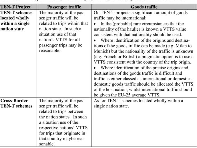
The implication of this is that users of the transport system should be allocated a willingness-to-pay that reflects incomes, journey lengths and trip purposes. This may result in attributing national VTTS values. Obviously a trade-off exists between sophistication and the practicality of implementing a sophisticated approach in any particular country. Additionally, the effort which the analyst endures to obtain values that represent the underlying willingness-to-pay should also reflect the scale of the scheme: Obviously greater efforts should be made for large schemes with significant capital costs than for small schemes, where reasonable ap-proximations to the underlying WTP maybe made. Some EU countries have well developed appraisal frameworks with large quantities of data available to the analyst whilst others do

(18)

S8

Summary HEATCO D5

not. In the latter situations it is unrealistic to expect scheme promoters to survey all the rele-vant data, therefore some values may have to be approximated and some may have to be imported from elsewhere. Appropriate assumptions will also have to be made in order to approximate the VTTS if the nationality or origins and destinations of traffic are unknown. The calculation of the economic benefits associated with travel time savings is very straight-forward. In essence it is the product of the five items of data:

(i) Demand - the number of passengers/vehicles/goods traffic making a particular origin-destination trip in the Scenario “Do Minimum” (D0) and in the Scenario “Do Something”

(D1);

(ii) Time saving – the time saving experienced by the users making that particular origin-destination trip (T0-T1); and

(iii)VTTS – the value of the travel time saving (for that segment of traffic)

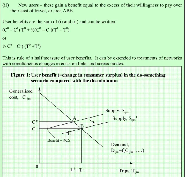
The travel time saving element of the consumer surplus for that origin-destination trip is calculated using the rule of a half (see Chapter 4):

½(D0+D1)*(T0-T1)*VTTS

The total user benefit from travel time savings is the sum of all time saving related consumer surpluses for all origin-destination movements.

Some vehicle operating cost models for commercial goods vehicles and business traffic in-clude the time elements of the journey (e.g. driver and crew wages). Care should be taken in such situations to avoid double counting this component in both time and vehicle operating cost benefits, both in modelling and appraisal.

It is our recommendation that modelling and appraisal values should reflect the same underly-ing willunderly-ingness-to-pay of the transport users and should only differ in their unit of account. Basing values of time within an appraisal on underlying willingness-to-pay has implications for the equitable treatment of people with different incomes within the appraisal framework. It is therefore recommended that the analyst in addition to reporting the aggregate monetised travel time savings benefits also reports the absolute time savings and the income brackets of the users to whom they accrue.

(19)

Table 0.3 Estimated VTTS values – work (business) passenger trips (€2002 per passenger per

hour, factor prices)

Business Country

Air Bus Car, Train

Austria 39.11 22.79 28.40 Belgium 37.79 22.03 27.44 Cyprus 29.04 16.92 21.08 Czech Republic 19.65 11.45 14.27 Denmark 43.43 25.31 31.54 Estonia 17.66 10.30 12.82 Finland 38.77 22.59 28.15 France 38.14 22.23 27.70 Germany 38.37 22.35 27.86 Greece 26.74 15.59 19.42 Hungary 18.62 10.85 13.52 Ireland 41.14 23.97 29.87 Italy 35.29 20.57 25.63 Latvia 16.15 9.41 11.73 Lithuania 15.95 9.29 11.58 Luxembourg 52.36 30.51 38.02 Malta 25.67 14.96 18.64 Netherlands 38.56 22.47 28.00 Poland 17.72 10.33 12.87 Portugal 26.63 15.52 19.34 Slovakia 17.02 9.92 12.36 Slovenia 25.88 15.08 18.80 Spain 30.77 17.93 22.34 Sweden 41.72 24.32 30.30 United Kingdom 39.97 23.29 29.02 EU (25 Countries) 32.80 19.11 23.82 Switzerland 45.41 26.47 32.97

(20)

S10

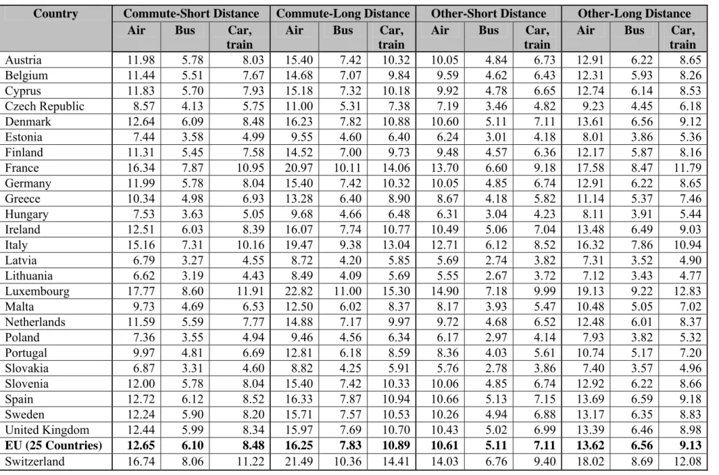
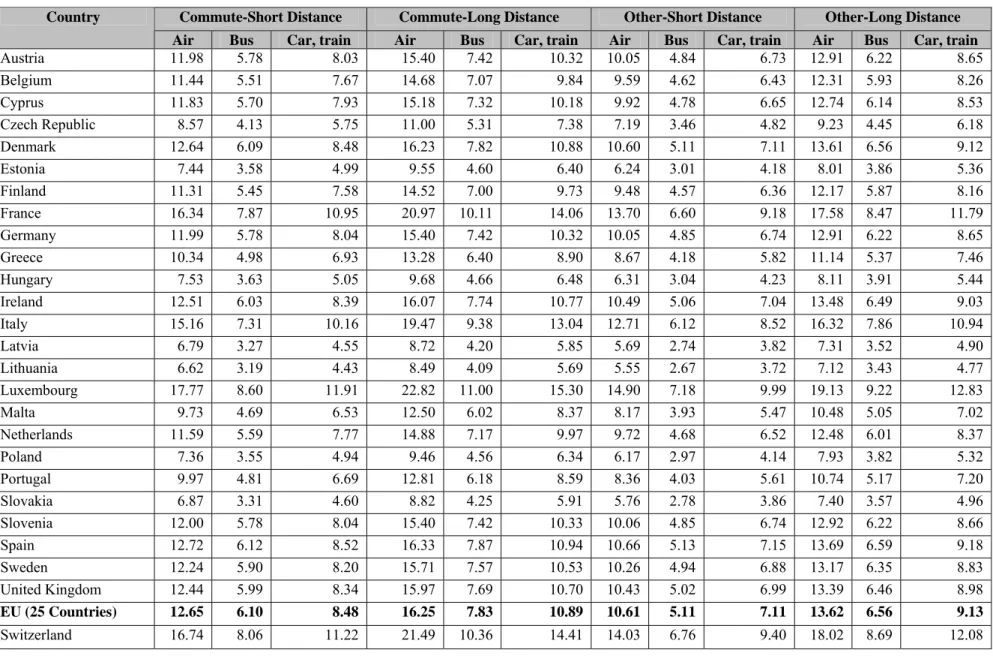
Table 0.4 Estimated VTTS values – non-work passenger trips (€2002 per passenger per hour, factor prices)

Commute-Short Distance Commute-Long Distance Other-Short Distance Other-Long Distance Country

Air Bus Car, train

Air Bus Car, train Austria 11.98 5.78 8.03 15.40 7.42 10.32 10.05 4.84 6.73 12.91 6.22 8.65 Belgium 11.44 5.51 7.67 14.68 7.07 9.84 9.59 4.62 6.43 12.31 5.93 8.26 Cyprus 11.83 5.70 7.93 15.18 7.32 10.18 9.92 4.78 6.65 12.74 6.14 8.53 Czech Republic 8.57 4.13 5.75 11.00 5.31 7.38 7.19 3.46 4.82 9.23 4.45 6.18 Denmark 12.64 6.09 8.48 16.23 7.82 10.88 10.60 5.11 7.11 13.61 6.56 9.12 Estonia 7.44 3.58 4.99 9.55 4.60 6.40 6.24 3.01 4.18 8.01 3.86 5.36 Finland 11.31 5.45 7.58 14.52 7.00 9.73 9.48 4.57 6.36 12.17 5.87 8.16 France 16.34 7.87 10.95 20.97 10.11 14.06 13.70 6.60 9.18 17.58 8.47 11.79 Germany 11.99 5.78 8.04 15.40 7.42 10.32 10.05 4.85 6.74 12.91 6.22 8.65 Greece 10.34 4.98 6.93 13.28 6.40 8.90 8.67 4.18 5.82 11.14 5.37 7.46 Hungary 7.53 3.63 5.05 9.68 4.66 6.48 6.31 3.04 4.23 8.11 3.91 5.44 Ireland 12.51 6.03 8.39 16.07 7.74 10.77 10.49 5.06 7.04 13.48 6.49 9.03 Italy 15.16 7.31 10.16 19.47 9.38 13.04 12.71 6.12 8.52 16.32 7.86 10.94 Latvia 6.79 3.27 4.55 8.72 4.20 5.85 5.69 2.74 3.82 7.31 3.52 4.90 Lithuania 6.62 3.19 4.43 8.49 4.09 5.69 5.55 2.67 3.72 7.12 3.43 4.77 Luxembourg 17.77 8.60 11.91 22.82 11.00 15.30 14.90 7.18 9.99 19.13 9.22 12.83 Malta 9.73 4.69 6.53 12.50 6.02 8.37 8.17 3.93 5.47 10.48 5.05 7.02 Netherlands 11.59 5.59 7.77 14.88 7.17 9.97 9.72 4.68 6.52 12.48 6.01 8.37 Poland 7.36 3.55 4.94 9.46 4.56 6.34 6.17 2.97 4.14 7.93 3.82 5.32 Portugal 9.97 4.81 6.69 12.81 6.18 8.59 8.36 4.03 5.61 10.74 5.17 7.20 Slovakia 6.87 3.31 4.60 8.82 4.25 5.91 5.76 2.78 3.86 7.40 3.57 4.96 Slovenia 12.00 5.78 8.04 15.40 7.42 10.33 10.06 4.85 6.74 12.92 6.22 8.66 Spain 12.72 6.12 8.52 16.33 7.87 10.94 10.66 5.13 7.15 13.69 6.59 9.18 Sweden 12.24 5.90 8.20 15.71 7.57 10.53 10.26 4.94 6.88 13.17 6.35 8.83 United Kingdom 12.44 5.99 8.34 15.97 7.69 10.70 10.43 5.02 6.99 13.39 6.46 8.98 EU (25 Countries) 12.65 6.10 8.48 16.25 7.83 10.89 10.61 5.11 7.11 13.62 6.56 9.13 Switzerland 16.74 8.06 11.22 21.49 10.36 14.41 14.03 6.76 9.40 18.02 8.69 12.08

(21)

Summary HEATCO D5

Table 0.5 Estimated VTTS values – freight trips (€2002 per freight tonne per hour, factor

prices)

Per tonne of freight carried1 Country Road Rail Austria 3.37 1.38 Belgium 3.29 1.35 Cyprus 2.73 1.12 Czech Republic 2.06 0.84 Denmark 3.63 1.49 Estonia 1.90 0.78 Finland 3.34 1.37 France 3.32 1.36 Germany 3.34 1.37 Greece 2.55 1.05 Hungary 1.99 0.82 Ireland 3.48 1.43 Italy 3.14 1.30 Latvia 1.78 0.73 Lithuania 1.76 0.72 Luxembourg 4.14 1.70 Malta 2.52 1.04 Netherlands 3.35 1.38 Poland 1.92 0.78 Portugal 2.58 1.06 Slovakia 1.86 0.77 Slovenia 2.51 1.03 Spain 2.84 1.17 Sweden 3.53 1.45 United Kingdom 3.42 1.40 EU (25 Countries) 2.98 1.22 Switzerland 3.75 1.54

1_{Value per tonne of freight carried and not for the maximum load of the vehicle or the weight}

(22)

S12

Summary HEATCO D5

Table 0.6 Estimated VTTS values – work (business) passenger trips (€2002 PPP per

passen-ger per hour, factor prices)

Business Country

Air Bus Car, train

Austria 37.50 21.85 27.23 Belgium 36.94 21.53 26.82 Cyprus 32.92 19.18 23.90 Czech Republic 36.59 21.31 26.57 Denmark 33.05 19.26 24.00 Estonia 31.76 18.52 23.07 Finland 34.61 20.17 25.13 France 36.57 21.31 26.56 Germany 34.53 20.12 25.07 Greece 34.07 19.86 24.74 Hungary 34.05 19.84 24.72 Ireland 35.43 20.65 25.73 Italy 36.91 21.51 26.81 Latvia 31.79 18.53 23.09 Lithuania 33.31 19.39 24.17 Luxembourg 46.14 26.88 33.50 Malta 36.99 21.56 26.85 Netherlands 36.13 21.06 26.24 Poland 32.34 18.85 23.48 Portugal 34.91 20.34 25.34 Slovakia 38.67 22.54 28.09 Slovenia 34.98 20.38 25.40 Spain 35.74 20.83 25.95 Sweden 35.24 20.54 25.59 United Kingdom 35.56 20.72 25.82 EU (25 Countries) 32.80 19.11 23.82 Switzerland 31.87 18.57 23.14

(23)

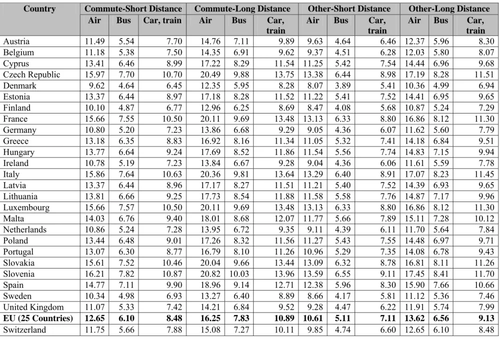
Summary HEATCO D5 Table 0.7 Estimated VTTS values – non-work passenger trips (€2002 PPP per passenger per hour, factor prices)

Commute-Short Distance Commute-Long Distance Other-Short Distance Other-Long Distance Country

Air Bus Car, train Air Bus Car, train

Air Bus Car, train

Air Bus Car, train Austria 11.49 5.54 7.70 14.76 7.11 9.89 9.63 4.64 6.46 12.37 5.96 8.30 Belgium 11.18 5.38 7.50 14.35 6.91 9.62 9.37 4.51 6.28 12.03 5.80 8.07 Cyprus 13.41 6.46 8.99 17.22 8.29 11.54 11.25 5.42 7.54 14.44 6.96 9.68 Czech Republic 15.97 7.70 10.70 20.49 9.88 13.75 13.38 6.44 8.98 17.19 8.28 11.51 Denmark 9.62 4.64 6.45 12.35 5.95 8.28 8.07 3.89 5.41 10.36 4.99 6.94 Estonia 13.37 6.44 8.97 17.18 8.28 11.52 11.22 5.41 7.52 14.41 6.95 9.65 Finland 10.10 4.87 6.77 12.96 6.25 8.69 8.47 4.08 5.68 10.87 5.24 7.29 France 15.66 7.55 10.50 20.11 9.69 13.48 13.13 6.33 8.80 16.86 8.12 11.30 Germany 10.80 5.20 7.23 13.86 6.68 9.29 9.05 4.36 6.07 11.62 5.60 7.79 Greece 13.18 6.35 8.83 16.92 8.16 11.34 11.05 5.32 7.41 14.18 6.84 9.51 Hungary 13.77 6.64 9.24 17.69 8.52 11.86 11.54 5.56 7.74 14.83 7.15 9.94 Ireland 10.78 5.19 7.23 13.84 6.67 9.28 9.04 4.36 6.06 11.61 5.59 7.78 Italy 15.86 7.64 10.63 20.36 9.81 13.64 13.29 6.40 8.91 17.07 8.23 11.45 Latvia 13.37 6.44 8.96 17.17 8.27 11.51 11.21 5.40 7.52 14.39 6.93 9.65 Lithuania 13.81 6.66 9.25 17.73 8.54 11.88 11.58 5.58 7.76 14.87 7.17 9.96 Luxembourg 15.66 7.57 10.50 20.11 9.69 13.48 13.13 6.33 8.80 16.86 8.12 11.30 Malta 14.03 6.76 9.40 18.01 8.68 12.07 11.77 5.66 7.89 15.11 7.28 10.12 Netherlands 10.86 5.24 7.28 13.95 6.72 9.35 9.11 4.39 6.11 11.70 5.64 7.84 Poland 13.44 6.48 9.01 17.26 8.32 11.56 11.27 5.43 7.55 14.48 6.97 9.71 Portugal 13.07 6.30 8.77 16.79 8.10 11.26 10.96 5.29 7.35 14.08 6.78 9.43 Slovakia 15.61 7.52 10.46 20.04 9.66 13.44 13.09 6.32 8.78 16.81 8.11 11.26 Slovenia 16.21 7.82 10.87 20.82 10.03 13.96 13.59 6.55 9.11 17.45 8.41 11.70 Spain 14.77 7.11 9.90 18.96 9.14 12.71 12.38 5.96 8.30 15.90 7.66 10.66 Sweden 10.34 4.98 6.93 13.27 6.40 8.89 8.66 4.17 5.81 11.12 5.36 7.46 United Kingdom 11.07 5.33 7.42 14.21 6.84 9.52 9.28 4.47 6.22 11.91 5.74 7.99

(24)

S14

Table 0.8 Estimated VTTS values – freight trips (€2002 PPP per freight tonne per hour, factor

prices)

Per tonne of freight carried1 Country Road Rail Austria 3.23 1.33 Belgium 3.22 1.32 Cyprus 3.10 1.27 Czech Republic 3.83 1.57 Denmark 2.76 1.14 Estonia 3.41 1.40 Finland 2.98 1.22 France 3.18 1.30 Germany 3.01 1.24 Greece 3.25 1.34 Hungary 3.64 1.49 Ireland 3.00 1.23 Italy 3.29 1.36 Latvia 3.50 1.43 Lithuania 3.67 1.50 Luxembourg 3.64 1.50 Malta 3.64 1.50 Netherlands 3.14 1.29 Poland 3.51 1.43 Portugal 3.39 1.39 Slovakia 4.24 1.74 Slovenia 3.39 1.39 Spain 3.30 1.36 Sweden 2.98 1.22 United Kingdom 3.04 1.25 EU (25 Countries) 2.98 1.22 Switzerland 2.63 1.08

1_{Value per tonne of freight carried and not for the maximum load of the vehicle or the weight}

of the vehicle.

0.4 Value of changes in accident risks

The recommendations given in the following, focus on a consistent set of monetary values for assessing accident risks and of factors for correcting underreporting for accident risks based on accident statistics. We assume that procedures for estimating accident risks for fatalities, severe and slight injuries have been established in the project planning process and are thus available for the appraisal.

(25)

We adopt a modified accident impact definition based on EUNET (Nellthorp et al. 1998)

• Fatality: death arising from the accident.

• Serious injury: casualties which require hospital treatment and have lasting injuries, but the victim does not die within the fatality recording period.

• Slight injury: casualties whose injuries do not require hospital treatment or, if they do, the effect of the injury quickly subsides.

• Damage-only accident: accident without casualties.

A 30 day period restriction for fatalities, as given in the original definition, is a pragmatic simplification for accident reporting, because it would be quite demanding to observe all severely injured persons for a longer time period, say e.g. 60 days. As there is evidence for considerable under-reporting due to the 30 day limit, we recommend correcting the available statistical data to include all fatalities due to accidents (see below).

It would be appropriate to distinguish at least between serious injuries entailing permanent invalidity and serious injuries where victims virtually recover entirely. However, often the necessary data are not available. Thus due to data limitations we recommend to use the EU-NET definition as default.

Underreporting of road accidents is a well recognized problem in official (road) accident statistics. Therefore, the official figures underestimate the true number of accidents. Based on a literature review, we conclude that underreporting of accidents is only relevant for road transport. We recommend to apply the correction factors for unreported accidents (= ratio all accidents / reported accidents) as given in Table 0.9. The correction factor given for fatalities of 1.02 should be applied in all countries alike, since here the problem is not underreporting, but that some victims die after expiry of the recording period of 30 days.

Table 0.9 Recommendation for European average correction factors for unreported road accidents.

Fatality Serious injury Slight injury Average injury Damage only

Average 1.02 1.50 3.00 2.25 6.00

Car 1.02 1.25 2.00 1.63 3.50

Motorbike/moped 1.02 1.55 3.20 2.38 6.50

Bicycle 1.02 2.75 8.00 5.38 18.50

Pedestrian 1.02 1.35 2.40 1.88 4.50

The valuation of an accident can be divided into direct economic costs, indirect economic costs and a value of safety per se. We recommend using values as follows:

a) Value of safety per se: WTP for safeguarding human life based on stated preference stud-ies carried out in the country concerned.

b) Direct and indirect economic costs (mainly medical and rehabilitation cost, administrative cost of legal system, and production losses): cost values for the country under assessment. c) Material damage from accidents: cost values for the average damage caused by accidents

(26)

S16

Summary HEATCO D5

If such values are not available for a) and b) the values provided in Table 0.10 may be used. The split into value of safety per se and economic costs is given in the main text. The values expressed in PPPs, show a much smaller range.

Since the uncertainties in estimating the value of safety per se are comparably large, we rec-ommend carrying out a sensitivity analysis for this value. Based on European Commission (2005) we recommend using v/3 as lower boundary and v*3 as high boundary of the sensitiv-ity analysis (with v = value of safety per se).

Wherever possible, the values used in demand modelling and valuation of effects should be consistent. If the values used in demand modelling comply with the requirements above, these should be used for valuation. If this is not the case the values, given in Table 0.10 should be used for demand modelling.

Table 0.10 Estimated values for casualties avoided.

Country Fatality Severe injury Slight injury Fatality Severe injury Slight injury

(€2002, factor prices) (€2002 PPP, factor prices)

Austria 1,760,000 240,300 19,000 1,685,000 230,100 18,200 Belgium 1,639,000 249,000 16,000 1,603,000 243,200 15,700 Cyprus 704,000 92,900 6,800 798,000 105,500 7,700 Czech Republic 495,000 67,100 4,800 932,000 125,200 9,100 Denmark 2,200,000 272,300 21,300 1,672,000 206,900 16,200 Estonia 352,000 46,500 3,400 630,000 84,400 6,100 Finland 1,738,000 230,600 17,300 1,548,000 205,900 15,400 France 1,617,000 225,800 17,000 1,548,000 216,300 16,200 Germany 1,661,000 229,400 18,600 1,493,000 206,500 16,700 Greece 836,000 109,500 8,400 1,069,000 139,700 10,700 Hungary 440,000 59,000 4,300 808,000 108,400 7,900 Ireland 2,134,000 270,100 20,700 1,836,000 232,600 17,800 Italy 1,430,000 183,700 14,100 1,493,000 191,900 14,700 Latvia 275,000 36,700 2,700 534,000 72,300 5,200 Lithuania 275,000 38,000 2,700 575,000 78,500 5,700 Luxembourg 2,332,000 363,700 21,900 2,055,000 320,200 19,300 Malta 1,001,000 127,800 9,500 1,445,000 183,500 13,700 Netherlands 1,782,000 236,600 19,000 1,672,000 221,500 17,900 Norway 2,893,000 406,000 29,100 2,055,000 288,300 20,700 Poland 341,000 46,500 3,300 630,000 84,500 6,100 Portugal 803,000 107,400 7,400 1,055,000 141,000 9,700 Slovakia 308,000 42,100 3,000 699,000 96,400 6,900 Slovenia 759,000 99,000 7,300 1,028,000 133,500 9,800 Spain 1,122,000 138,900 10,500 1,302,000 161,800 12,200 Sweden 1,870,000 273,300 19,700 1,576,000 231,300 16,600 Switzerland 2,574,000 353,800 27,100 1,809,000 248,000 19,100 United Kingdom 1,815,000 235,100 18,600 1,617,000 208,900 16,600 Notes: Value of safety per se based on UNITE (see Nellthorp et al., 2001): fatality €1.50 million (market price 1998 – €1.25 million factor costs 2002); severe/slight injury 0.13/0.01 of fatality; Direct and indirect economic costs: fatality 0.10 of value of safety per se; severe and slight injury based on European Commission (1994).

(27)

We recommend increasing values for future years based on a default inter-temporal elasticity to GDP per capita growth of 1.0. If accident costs prove to contribute an important part of the benefits quantified in an assessment, we recommend sensitivity testing with an income elas-ticity of 0.7.

Please note that the assumption of linearly growing values clearly requires explicit and careful demand modelling over time. If this is not the case, the results are likely to overestimate benefits from a transport project.

The recommended calculation procedure is as follows:

Step 1: quantification of changes in the number of fatalities, serious injuries, slight inju-ries, and material damage due to a project using local or national risk functions. Step 2: adjustment for underreporting of casualties with national (if available) or

Euro-pean factors.

Step 3: preparation of the cost factor table by increasing the cost factor according to the assumed country-specific GDP per capita growth for each year of the analysis. Step 4: multiplication of casualties with cost factors.

Step 5: reporting of casualties and costs.

0.5 Environmental costs

Our general recommendation is – wherever possible – to value impacts, not environmental burden (for example value mortality risks caused by PM10 emissions and not the emissions of

PM10) and to monetise impacts as far as possible using values based on the WTP concept. To

increase transparency and allow for alternative valuations both costs and (key) impacts should be reported.

In the following sections we provide values that can be used if no country-specific state-of-the art values are available for calculating environmental costs due to air pollution, noise and global warming.

0.5.1 Air pollution

We recommend using country-specific values taking into account local population density and regional climate. Cost factors measured in € per tonne of pollutant emitted in different environments (urban areas, outside built-up areas) are provided below. The list of pollutants should cover

• primary PM2.5 for transport emissions (PM10 for emissions from power plants), • NOx as precursor of nitrate aerosols and ozone,

• SO2 for direct effects and as precursor of sulphate aerosols, and • NMVOC as precursor of ozone.

(28)

S18

Summary HEATCO D5

Project related emissions should be calculated using national emission factors; if such factors are not available, emission factors from international sources can be applied, taking into account national vehicle fleet compositions as far as possible.

Existing research identified damage to human health as the most important effect in terms of quantifiable costs. In particular the reduction of life expectancy in terms of Years of Life Lost (YOLL) contributes to health costs. Therefore, YOLL is a good indicator for physical impacts caused.

Table 0.11 presents the recommended cost factors in € per tonne of pollutant emitted by road and other ground level transport (e.g. diesel trains), Please note however, that the monetary values given do not only assess YOLLs, but include a number of other health impacts and in addition damage to crops and materials. Table 0.13 presents the impact factors. The corre-sponding values for high stack emissions from electricity production in power plants are given in the main text.

The cost factors are estimated average values based on the spatial distribution of emissions within a country. The impacts and costs may vary within one country, particularly in large ones. The variation in costs due to NOx, NMVOC and SO2 between countries is mainly

caused by air chemistry (incl. ozone formation) and the population affected. For primary particulates no air chemistry is involved, therefore differences reflect the number of popula-tion affected, which is determined mainly by distance to the emission source and the prevail-ing wind direction.

The PPP adjusted values in Table 0.12 differ from the values in Table 0.11 only for costs due to primary particle emissions. NOx, NMVOC and SO2 have virtually no local effects as most

of their impact is caused after chemical transformation to other substances (ammonium ni-trates and sulphates, ozone); damages occur far from the emission source, mostly in other countries. For keeping modelling effort reasonable trans-boundary impacts are valued at European average values. Rounding masks differences between € and PPP results. In contrast, for primary particles local effects play an important role, therefore the PPP weighted cost factors differ from those expressed in real €.

(29)

Table 0.11 Cost factors for road transport emissions* per tonne of pollutant emitted in €2002

(factor prices).

Pollutant emitted NOx NMVOC SO2 PM2.5

Effective pollutant O3, Nitrates,

Crops

O3 Sulphates, Acid

deposition, Crops

primary PM2.5

Local environment urban outside built-up areas

Austria 4,300 600 3,900 450,000 73,000 Belgium 2,700 1,100 5,400 440,000 95,000 Cyprus** 500 1,100 500 230,000 20,000 Czech Republic 3,200 1,100 4,100 170,000 61,000 Denmark 1,800 800 1,900 520,000 54,000 Estonia 1,400 500 1,200 100,000 23,000 Finland 900 200 600 400,000 33,000 France 4,600 800 4,300 430,000 83,000 Germany 3,100 1,100 4,500 430,000 80,000 Greece 2,200 600 1,400 210,000 34,000 Hungary 5,000 800 4,100 150,000 54,000 Ireland 2,000 400 1,600 510,000 50,000 Italy 3,200 1,600 3,500 370,000 70,000 Latvia 1,800 500 1,400 80,000 22,000 Lithuania 2,600 500 1,800 90,000 28,000 Luxemburg 4,800 1,400 4,900 590,000 96,000 Malta (O3 estimated) 500 1,100 500 170,000 16,000 Netherlands 2,600 1,000 5,000 470,000 88,000 Poland 3,000 800 3,500 130,000 53,000 Portugal 2,800 1,000 1,900 210,000 37,000 Slovakia 4,600 1,100 3,800 110,000 49,000 Slovenia 4,400 700 4,000 220,000 55,000 Spain 2,700 500 2,100 280,000 41,000 Sweden 1,300 300 1,000 440,000 40,000 Switzerland 4,500 600 3,900 640,000 86,000 United Kingdom 1,600 700 2,900 450,000 67,000

Notes: Cost categories included are: human health, crop losses, material damages. * Values are applicable to all emissions at ground level (e.g. diesel locomotives). ** Estimated values as Cyprus outside of modelling domain.

(30)

S20

Summary HEATCO D5

Table 0.12 Cost factors for road transport emissions* per tonne of pollutant emitted in €2002

PPP(factor prices).

Effective pollutant O3, Nitrates,

Crops

O3 Sulphates, Acid

deposition, Crops

primary PM2.5

Austria 4,300 600 3,900 430,000 72,000 Belgium 2,700 1,100 5,400 440,000 95,000 Cyprus** 500 1,100 500 260,000 22,000 Czech Republic 3,200 1,100 4,100 270,000 67,000 Denmark 1,800 800 1,900 400,000 47,000 Estonia 1,400 500 1,200 160,000 27,000 Finland 900 200 600 360,000 30,000 France 4,600 800 4,300 410,000 82,000 Germany 3,100 1,100 4,500 400,000 78,000 Greece 2,200 600 1,400 270,000 38,000 Hungary 5,000 800 4,100 230,000 59,000 Ireland 2,000 400 1,600 440,000 46,000 Italy 3,200 1,600 3,500 390,000 71,000 Latvia 1,800 500 1,400 140,000 26,000 Lithuania 2,600 500 1,800 160,000 32,000 Luxemburg 4,800 1,400 4,900 730,000 104,000 Malta (O3 estimated) 500 1,100 500 240,000 20,000 Netherlands 2,600 1,000 5,000 440,000 86,000 Poland 3,000 800 3,500 190,000 57,000 Portugal 2,800 1,000 1,900 270,000 40,000 Slovakia 4,600 1,100 3,800 200,000 54,000 Slovenia 4,400 700 4,000 280,000 58,000 Spain 2,700 500 2,100 320,000 44,000 Sweden 1,300 300 1,000 370,000 36,000 Switzerland 4,500 600 3,900 460,000 76,000 United Kingdom 1,600 700 2,900 410,000 64,000

Notes: Cost categories included are: human health, crop losses, material damages. * Values are applicable to all emissions at ground level (e.g. diesel locomotives). ** Estimated values as Cyprus outside of modelling domain.

(31)

Table 0.13 Impact factors for road transport emissions* (lost life expectancy in years of life lost per 1000 tonnes of pollutant emitted).

Effective pollutant O3, Nitrates O3 Sulphates primary PM2.5

Austria 61 0.6 58 5,800 1,080 Belgium 57 1.3 81 6,200 1,470 Cyprus** 8 0.5 8 5,100 400 Czech Republic 50 1.0 58 5,900 1,180 Denmark 29 0.9 28 5,400 680 Estonia 18 1.5 17 5,300 590 Finland 11 0.2 9 5,100 450 France 65 0.8 65 6,000 1,280 Germany 53 1.2 65 5,900 1,220 Greece 20 0.2 20 5,400 670 Hungary 63 0.6 58 5,800 1,080 Ireland 30 0.7 25 5,300 640 Italy 50 0.8 54 5,800 1,120 Latvia 22 0.9 21 5,300 590 Lithuania 29 0.9 26 5,400 690 Luxemburg 70 1.5 73 6,000 1,330 Malta (O3 estimated) 8 0.5 8 5,100 400 Netherlands 56 1.1 74 6,000 1,320 Poland 46 0.8 49 5,800 1,070 Portugal 31 0.5 30 5,400 720 Slovakia 57 1.0 55 5,700 1,020 Slovenia 63 0.5 59 5,700 1,020 Spain 34 0.4 33 5,400 720 Sweden 15 0.4 15 5,200 530 Switzerland 68 0.7 59 5,800 1,120 United Kingdom 35 1.0 44 5,700 980

Notes: * values are applicable to all emissions at ground level (e.g. diesel locomotives). ** Estimated values as Cyprus outside of modelling domain.

We recommend increasing values for future years based on a default inter-temporal elasticity to GDP per capita growth of 1.0. If air pollution costs prove to contribute an important part of the benefits quantified in an assessment we recommend sensitivity testing with an income elasticity of 0.7.

Please note that the assumption of linearly growing values over time clearly requires explicit and careful emission modelling over time. If this is not the case, the results are likely to over-estimate benefits from a transport project, as vehicle emissions can be assumed to decrease considerably in the future. Information on the future development of emission factors can be found for instance at http://www.tremove.org/download/index.htm.

(32)

S22

Summary HEATCO D5

Step 1: quantification of change in pollutant emissions (NOx, SO2, NMVOC,

PM2.5/PM10) due to a project, measured in tonnes, using state-of-the-art national

or European emission factors.

Step 2: classification of emissions according to height of emission sources (ground-level vs. high stack) and local environment (urban – outside built-up areas). Ground level emissions are released from internal combustion engines, high stack emis-sions are released during electricity production in power plants.

Step 3: preparation of the cost factor table by increasing the cost factor according to the assumed country-specific GDP per capita growth for each year of the analysis. Step 4: calculation of impacts (multiplication of pollutant emissions by impact factor)

and costs (multiplication of pollutant emissions by cost factor). Step 5: reporting of impacts and costs.

0.5.2 Noise

For noise costs it is suggested to use country-specific values per person exposed to a certain noise level (see Table 0.14). The suggested impact indicator, which should be reported along-side with the monetary results, is the number of persons highly annoyed – see Table 0.15. We recommend increasing monetary values for future years based on a default inter-temporal elasticity to GDP per capita growth of 1.0. If noise costs prove to contribute an important part of the benefits quantified in an assessment we recommend sensitivity testing with an income elasticity of 0.7.

Please note that the assumption of linearly growing values over time clearly requires explicit and careful emission modelling over time. If this is not the case, the results are likely to over-estimate benefits from a transport project, as vehicle emissions are likely to decrease in the future.

Step 1: quantification of the number of persons exposed to certain noise levels (should be available from noise calculations) for the Minimum case and the Do-Something case.

Step 2: preparation of the cost factor table by increasing the cost factor according to the assumed country-specific GDP per capita growth for each year of the analysis. Step 3: calculation of impacts (multiply percentage of highly annoyed persons by

num-ber of persons exposed) and costs (multiply cost per person by numnum-ber of per-sons exposed) for both cases.

Step 4: subtraction of total costs for the Do-Something case from Do-Minimum case Step 5: reporting of costs and impacts (change in number of people highly annoyed).

(33)

Table 0.14 Cost factors for noise exposure for Finland (€2002, factor costs, per year per person

exposed; to derive €2002 PPP the values below are divided by the Finish PPP

ad-justment factor of 1.12). For values for all countries see main text.

Finland Central values New approach High values

Lden (dB(A)) Road Rail Aircraft Road Rail Aircraft Road Rail Aircraft

≥43 0 0 0 6 3 10 0 0 0 ≥44 0 0 0 6 3 11 0 0 0 ≥45 0 0 0 7 3 12 0 0 0 ≥46 0 0 0 8 4 14 0 0 0 ≥47 0 0 0 9 4 15 0 0 0 ≥48 0 0 0 10 5 16 0 0 0 ≥49 0 0 0 11 6 18 0 0 0 ≥50 0 0 0 12 6 19 0 0 0 ≥51 10 0 16 13 7 20 23 0 36 ≥52 20 0 32 14 7 22 47 0 72 ≥53 31 0 47 15 8 23 70 0 108 ≥54 41 0 63 17 9 25 93 0 144 ≥55 51 0 79 18 10 26 116 0 180 ≥56 61 10 95 19 10 27 140 23 216 ≥57 71 20 110 20 11 29 163 47 252 ≥58 81 31 126 22 12 30 186 70 288 ≥59 92 41 142 23 13 32 209 93 324 ≥60 102 51 158 24 14 33 233 116 360 ≥61 112 61 174 26 15 35 256 140 397 ≥62 122 71 189 27 16 36 279 163 433 ≥63 132 81 205 29 17 38 302 186 469 ≥64 143 92 221 30 18 39 326 209 505 ≥65 153 102 237 32 19 40 349 233 541 ≥66 163 112 252 33 20 42 372 256 577 ≥67 173 122 268 35 21 43 395 279 613 ≥68 183 132 284 36 22 45 419 302 649 ≥69 193 143 300 38 23 46 442 326 685 ≥70 204 153 316 40 24 48 465 349 721 ≥71 270 219 388 98 82 106 545 429 813 ≥72 287 236 410 106 90 114 575 459 856 ≥73 304 253 433 115 98 122 605 489 899 ≥74 321 270 456 123 106 130 635 519 942 ≥75 338 287 478 132 114 139 665 549 985 ≥76 355 305 501 140 122 147 695 579 1028 ≥77 372 322 524 149 131 155 725 609 1071 ≥78 390 339 546 158 139 163 756 639 1114 ≥79 407 356 569 166 147 172 786 669 1157 ≥80 424 373 592 175 155 180 816 700 1200 ≥81 441 390 614 183 164 188 846 730 1242

Notes: All values include health effects and annoyance. Central values comprise the WTP for reducing annoy-ance based on stated preference studies (see Working group on health and socio-economic aspects, 2003). For “New approach” annoyance was based on dose-response functions; monetary values were taken from the HEATCO surveys (see Navrud et al. 2006). High values include annoyance valuation based on he-donic pricing as applied in UNITE (see Bickel et al. 2003).

(34)

S24

Summary HEATCO D5

Table 0.15 Impact indicator for noise exposure: percentage of adult persons highly annoyed per person (all ages) exposed – based on functions given in European Commission (2002), assuming 80% of population are adults.

Lden Road Rail Aircraft

dB(A) % % % ≥43 0.4 0.1 0.3 ≥44 0.8 0.3 0.6 ≥45 1.1 0.4 1.0 ≥46 1.5 0.5 1.4 ≥47 1.9 0.6 2.0 ≥48 2.2 0.7 2.5 ≥49 2.6 0.8 3.2 ≥50 2.9 1.0 3.9 ≥51 3.3 1.1 4.6 ≥52 3.7 1.3 5.4 ≥53 4.2 1.5 6.3 ≥54 4.6 1.7 7.2 ≥55 5.1 2.0 8.2 ≥56 5.6 2.3 9.3 ≥57 6.2 2.6 10.4 ≥58 6.8 2.9 11.5 ≥59 7.5 3.3 12.7 ≥60 8.3 3.8 14.0 ≥61 9.0 4.3 15.3 ≥62 9.9 4.8 16.7 ≥63 10.8 5.4 18.1 ≥64 11.9 6.1 19.6 ≥65 12.9 6.8 21.2 ≥66 14.1 7.6 22.7 ≥67 15.4 8.5 24.4 ≥68 16.8 9.5 26.1 ≥69 18.2 10.5 27.8 ≥70 19.8 11.6 29.6 ≥71 21.5 12.8 31.5 ≥72 23.3 14.1 33.4 ≥73 25.2 15.4 35.3 ≥74 27.2 16.9 37.3 ≥75 29.4 18.4 39.4 ≥76 31.7 20.1 41.5 ≥77 34.1 21.9 43.6 ≥78 36.7 23.8 45.8 ≥79 39.4 25.8 48.0 ≥80 42.3 27.9 50.3 ≥81 45.3 30.1 52.6