Antagonistic structural patterns in complex networks

Mar´ıa J. Palazzi,1_{Javier Borge-Holthoefer,}1 _{Claudio J. Tessone,}2 _{and Albert Sol´e-Ribalta}1 1_{Internet Interdisciplinary Institute (IN3), Universitat Oberta de Catalunya, Barcelona, Catalonia, Spain}

2_{URPP Social Networks, Universit¨at Z¨urich, Switzerland}

Identifying and explaining the structure of complex networks at different scales has become an important problem across disciplines. At the mesoscale, modular architecture has attracted most of the attention. At the macroscale, other arrangements –e.g. nestedness or core-periphery– have been studied in parallel, but to a much lesser extent. However, empirical evidence increasingly suggests that characterizing a network with a unique pattern typology may be too simplistic, since a system can integrate properties from distinct organizations at different scales. Here, we explore the relationship between some of those organizational patterns: two at the mesoscale (modularity and in-block nestedness); and one at the macroscale (nestedness). We analytically show that nestedness can be used to provide approximate bounds for modularity, with exact results in an idealized scenario. Specifically, we show that nestedness and modularity are antagonistic. Furthermore, we evince that in-block nestedness provides a parsimonious transition between nested and modular networks, taking properties of both. Far from a mere theoretical exercise, understanding the boundaries that discriminate each architecture is fundamental, to the extent modularity and nestedness are known to place heavy constraints on the stability of several dynamical processes, specially in ecology.

PACS numbers: 89.65.-s, 89.75.Fb,

The detection and identification of emergent structural pat-terns has been a main focus in the development of modern network theory. Such interest is not surprising, because these arrangements lie at the core of the discipline as one of the keys to the origins –which are the assembly rules that led to an ob-served pattern?– and dynamics –how is the system’s activity constrained by the structure?– of a network. In addition to these essential questions, the identification of structural sig-natures is a difficult taskper se, which explains as well why so much attention has been put on the technical problem.

Undoubtedly, in this context, modularity [1, 2] stands out: the organization of a network as a set of cohesive subgroups has, by far, concentrated most of the efforts [3–7]. Modular architecture is widespread [8–12] and responds to the intu-ition that similar elements in a complex system tend to flock together. However, there are other architectural principles be-yond community structure which may play more important roles. In ecology, for instance, scholars have faced the need to define and quantify other patterns, demonstrated to be more relevant in certain scenarios. This is the case of nestedness [13, 14], a concept that has been crucial to understand the stability and diversity of ecological systems [15, 16]. Other, more intricate, possibilities have also been explored [17, 18], like core-periphery structures [19, 20] –and its extension to the mesoscale [21]– are good examples of comparatively less studied architectures.

In these settings, the accent has been mainly placed on designing heuristics and improving algorithms [12, 20, 22]; understanding the dynamical constraints that those patterns impose [23, 24]; or describing plausible microscopic rules that make those patterns emerge [15, 25–27]. However, we have very limited knowledge on how different structural sig-natures may be intertwined, or how –if ever– they affect and limit each other. Indeed, we have examples in which two or more structural features (say, nestedness and modularity) have been jointly considered [28–31]. But such consideration over-looked to what extent the inherent constraints of one pattern

limit –or boost– the presence of the other. Furthermore, there is extensive evidence that modular and nested architectures play a critical role in relation to the stability of the dynam-ics of ecological systems [15, 16, 32, 33], economdynam-ics [34, 35] and social sciences [31]. Thus, understanding the possibility of coexistence of these structural patterns may shed light on the dynamical trade-offs that either arrangement can facilitate. In [31], the authors observe that modularity and nested-ness exhibit an anti-correlated behavior, suggesting that, at least in empirical data, these arrangements hardly coexist. In this work, we depart from this shallow evidence to first ex-plore experimentally, and then analytically, the structural re-lationship between three structural patterns: nestedness on the macroscopic side, modularity and in-block nestedness at the mesoscale. We analytically characterize these measures in an idealized family of networks, which allows us to precisely de-rive to what extent the macroscale organization places strict bounds to the emergence of mesoscale patterns. Eventually, we provide soft bound estimations for less restricted scenar-ios,i.e.real networks.

In a perfectly nested network, the set of neighbors of lower degree nodes are a subset of those with larger degree [36]. Such network is typically represented by a presence-absence matrixaij, and the degree of nestednessN, can be formally

defined as [37] N = 2 NT    NT X ij _O ij− hOiji kj(NT −1)Θ(ki−kj) _ , (1)

whereOij =Pkaikajkquantifies the overlap between nodes

iandj;kicorresponds to the degree of nodei; andΘ(·)is the

Heaviside step function, that ensures thatOij has a positive

contribution whenki ≥kj. Additionally,Oijis conveniently

corrected by a null model that discounts the expected overlap if links where drawn randomly,hOiji. NT is the size of the

network.

2 A modular structure is a rather ubiquitous mesoscale

struc-tural organization in which nodes are organized forming groups, i.e. devoting many links to nodes in the same group, and fewer links towards nodes outside. One of the most popu-lar methods to identify communities is through the maximiza-tion of the modularityQ [1]. The original equation can be

rewritten as Q= B X c=1 " lc L − _d c 2L 2# , (2)

whereBis the number of communities,Lis the total number

of links in the network,lcis the total number of links in

com-munityc, anddcis the sum of the degrees of all nodes in such

community.

The possibility of a combined nested-modular organization has been debated in different contexts [37–39]. One conceiv-able form of coexistence is in terms of hybrid structures, as described by Lewinsohnet al. in [17]. The general layout of these networks is modular, but interactions within each mod-ule (or block) are expected to be nested. In contrast, modular-ity makes no assumption on the internal organization of com-munities. Worth highlighting, this hybrid structure reframes nestedness, originally a macroscale feature, to the mesoscopic level –it can now be interpreted as an in-block nested structure withB = 1. The degree of in-block nestedness of a network

I[37] can be computed as I = 2 NT    NT X i,j _O ij− hOiji kj(Ci−1) Θ(ki−kj)δ(αi, αj) _ . (3)

Here,αirepresents the community nodeibelongs to, andCi

its size. δ(αi, αj)corresponds to the Kronecker delta, equal

to one only if nodesiandjbelong to the same community. In order to experimentally assess the dependence between the different presented structural measures, we rely on a prob-abilistic network generation model [37]. This model is able to generate structures (with and without noise) that smoothly interpolate between the different structural patterns of interest by recourse of 4 parameters: the number of modulesB, the fraction of inter-modular linksµ(inter-block noise), the frac-tion of links outside the perfect nested structurep(intra-block

noise), and the shape of the nested structureξ(cf.

Supplemen-tal Material).

We have measured _N, and optimized Qand _I for more

than2_×105 _{networks on a wide range of parameters: B}

∈

[1,9];ξ_∈[1.5,7];p_∈ [0,0.6]; andµ_∈[0,0.6]. Restricting

pandµ to0.6 allows us to introduce a high level of noise while still preserving some underlying mesoscale structure. For modularity and in-block nestedness optimization, we have used the extremal optimization algorithm [3], adapted to the corresponding objective functions (Eqs. 2 and 3, respectively). Community size ofNB = 50was assumed, so as we add

communities we are also increasing the size of the network, the total number of nodes being NT = BNB. Fixing NT

and reducing the size of the communities while increasingB

produces equivalent results.

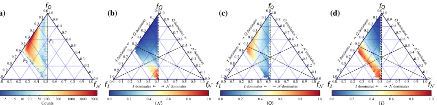
Figure 1 shows the results represented over four ternary heatmap plots. A ternary plot, or simplex, is a three-variable diagram in which the sum of the variables is a constant –1 in this case– (for further details cf. Supplemental Material). Panel (a) shows a density plot of the generated networks over the simplex, and the colorbar indicates the amount of net-works in each bin of the ternary plot. Relying on these results, it is apparent that the most frequent architecture is predom-inantly modular. This is expected since most generated net-works have blocks (B >1), and in-block nested networks are more restrictive, in terms of internal organization, than modu-lar ones. The color code in panels (b), (c) and (d) reports the average absolute value of_N, Qand_I. Dashed black lines

have been added as visual aids to evincedominanceregions. A quick glance already shows that the highest values ofN

andQnever overlap, whileIbridges between them. This is a valuable insight for the analytical results in the remainder of the article.

Another outstanding feature in Fig. 1 is the existence of sharp boundaries in the ternary plots. The first boundary,F1in

panel (a), is induced by the definitions ofN andI: as stated, Eq. 3 reduces to Eq. 1 whenB = 1. Translated to coordinates on the simplex,F1simply reflects that the contribution ofN

is always equal or smaller than the contribution ofI,f_{N ≤} f_I. More interesting, however, is the existence ofF2, which

suggests that there is an inherent limit that prohibits in-block nestedness to dominate further overQ. On close inspection

(see Fig. S3 of the Supplemental Materials), networks which map ontoF2have high values ofξand very low values ofp

andµ. We build on this finding to construct our analytical approach below.

The specific configuration of parameters alongF2in Fig. 1

points at a well-defined family of network configurations: a ring of star graphs,Gs hereafter. Indeed, an extreme shape

parameter (ξ → ∞), perfectly nested intra-block structure (p = 0) and minimum inter-block connectivity (µ ≈ 0) to guarantee a single giant component, render a network model which depends only onB, ranging from a single star (B= 1) to a set of stars (B >1) connected with a single link through their central nodes. In other words,Gsprovides the closest

compatible network architecture for the boundaryF2. Given

a ring of star graphs withBcommunities andNB nodes per

community, we can analytically derive the exact valuesN,I

andQ.

Nestedness. We obtain the analytical expression for N

from the expression in Eq. 1. The pair overlap of a generalist node (the center of each star subgraph),g, with a specialist

node (periphery of a star),s, isOgs/ks= 1ifgandsbelong

to the same star (and 0 otherwise). For all those pairs (regard-less of the star they belong to), the null model contribution is

hOgs/ksi= (NB+ 1)/BNB. We can obtain in a similar way

the terms for the the generalist-generalist pairs between stars. Summing up all the contributions, the final expression forN

is: N = BN 3 B−BNB2 −3BNB+B+ 2NB+ 2 BNB(BNB2 +BNB−NB−1) . (4)

(a) (b) (c) (d)

FIG. 1. Panel (a) shows the distribution of the generated networks over the ternary plot. The color bar indicates the amounts of networks in each bin. Panels (b), (c) and (d) show the average absolute value ofN,QandI, respectively.

Modularity. While the optimal partition for an arbitrary network cannot be easily obtained, this is not the case forGs

where each star in the ring forms a community. Thus, we can easily derive the contribution of each star to the totalQ

following Eq. 2. The first element islc=NB−1. The second

element (the amount of links of the network) includes links within and between communities,L = B(NB −1) +B =

BNB. The last term, the sum of the degrees of all the nodes in

communityc, corresponds todc = 2NB. Assembling these,

we obtain the modularity ofGsas

Q=B " NB−1 BNB − _2N B 2BNB 2# = 1₋ 1 NB − 1 B, (5)

which is equivalent to the general expression derived in [40]. In-block nestedness. The derivation ofIresembles that of

N, with the difference that only nodes within the same com-munity contribute; thus, all stars have the same contribution. Focusing now on each star, we have only two contributing terms to the sum: the pair overlap between specialist nodes,

s, and the pair overlap of the generalist node,g, with the spe-cialists. In both cases, the contribution is 1. The null model corrections arehOgsi=kgks/BNB = (NB+ 1)/BNBand

hOssi=ksks/BNB= 1/BNB. Finally, the size of the

com-munities isCg =Cs=NB. Replacing all the contributions

in Eq. 3, we obtain I= 1₋ 3 BNB − 2 NB . (6)

All the expressions presented above were obtained consid-ering a closed ring, on which the number of intercommunity links isB. For the casesB = 1andB = 2, the number of intercommunity links isB₋1and the degree of the generalist nodes iskg =NB−1andkg =NB, respectively (cf.

Sup-plemental Materials for details on these cases).

We now focus on the bounds that_N andQimpose on each

other in some important limits. These correspond to scenarios in which the number of blocks,B, and the size of the blocks,

NB, tend to∞.

We start withNB → ∞. In this case, Eqs. 4 and 5 reduce

to lim NB→∞N = 1 B, NBlim→∞ Q= 1−_B1, (7)

which implies that, under these circumstances,N andQare complementary –in accordance with the empirical results in [31]. This result proves analytically the antagonism that exists between these two structural patterns.

With respect to the caseB _{→ ∞}, Eqs. 4 and 5 turn now

lim

B→∞N = 0, Blim→∞Q=

NB−1

NB

. (8)

These results fit the expectation that, with increasingB, the

negative contribution of non-overlapping nodes through the null model overcomes the decreasing positive contributions realized.

Finally, with respect to in-block nestedness, the analytical calculations in both limits yield

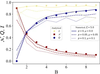
lim NB→∞I = 1 lim B→∞I= NB−2 NB (9) Noteworthy, the generated synthetic networks follow closely the predictions in limiting cases: Fig. 2 reports the analytical estimation of_N,Qand_I(Eqs. 4-6, symbols in the

figure) againstB, and the numerical results for networks gen-erated under different parameters. As the gengen-erated networks deviate from the ring of starsGs(i.e.p >0andµ > 0),

re-sults show a worse fit to the analytical prediction. The mutual bounds that_N andQimpose on each other are obvious,

ob-serving a perfectly anti-correlated behavior between nested-ness and modularity. Finally, as the networks transition from a nested (B= 1) to a modular (B >1) architecture, the values of in-block nestedness remain very high and almost constant. The previous results open a new front to understand the co-occurrence of macro- and mesoscale patterns in complex net-works. Complementary to the inherent limits ofQ[40, 41], we have now evidence that a certain connectivity arrangement (i.e. nestedness) places hard limits to modularity, at least in extreme settings. This certainty paves the way to obtain esti-mations forQprior to computationally costly endeavors:

in-deed, relaxing those conditions to realistic parameters, soft bounds forQmay be defined. The derivation of these bounds are presented below.

We start from aGsof sizeNT =BNB. From here, Eq. 4

can be rewritten in terms ofNT andB, and an estimation on

the number of blocks as a function ofN andNT can be

ob-tained, i.e.B∗ _{= f(N, N}

4

2

4

6

8

B

0.0

0.2

0.4

0.6

0.8

1.0



,

Q

,



FIG. 2. Comparison of the analytical (symbols) and numerical (lines) values ofN,Q,Iwith respect toB. All the calculations were per-formed by takingNB = 50andξ = 5. The values forpandµ

parameters are indicated in the plot legend.

Iare thus readily available, applyingB∗_{to Eqs. 4-5, i.e.} as-suming that the network structure lies on the boundary F2.

With the actual measure ofN, and upper estimations forQ

andI, we can obtain the relative fraction that each measure contributes to the ternary plot along theF2boundary,f_N↑,fQ↑

andf_I↑.

To obtain the lower bounds for Q, we observe from

Fig. 1(b) that, if we move from boundaryF2to boundaryF1

on thefQ-axis direction, i.e. horizontally in Fig. 1, theN

val-ues are approximately constant with respect to the contribu-tions ofQ(f_Q↑ andf_Q↓). This allows us to make an approxi-mation for the contributions ofQin the ternary plot atF1as

f_Q↓ ≈ f_Q↑. Additionally, we know thatN = I at boundary

F1. Thus,

f_Q↓ = Q

Q+I+N =

Q

Q+ 2N, (10)

from which a lower bound forQcan be obtained.

Figure 3 shows the values ofQas a function ofN for the previous synthetic ensemble (_∼2_×105_{networks; panel (a),}

grey dots); and 57 real unipartite networks (panel (b), red dots) [37]. In panel (a), the values of the theoretical upper and lower bounds are plotted in colors, the color bar indicating the net-work size. Our approximation ofQbounds is in good

agree-ment with actual values obtained after optimization: most of

the optimizedQvalues lie within the estimated soft bounds.

Despite the wide range of parameters –clearly far from limit-ing cases– estimated upper bounds behave likeQ = 1_{− N} almost perfectly. While these bounds are trivial forN ≈ 0, we observe that intermediate values of nestedness provide rel-evant information about the possible mesoscale organization of the network. Qvalues above the upper bound correspond

to networks with a single communityB = 1 and perfectly nested structure,p= 0 (see Fig. S4). These networks –less than 0.1% of the total– are dense enough to allow a partition

withB >1where the nodes of higher degree are gathered in a

block, resulting in values ofQlarger than expected [37].

Val-ues below the lower bound approximation are more numerous –although still a small fraction of the total. This imprecision shows that there is room to improve the underlying assump-tion, i.e. thatN values are constant with respect to the con-tributions ofQ. In the same spirit, upper and lower bounds

for_Ican be as well approximated from the actual value of_N (see Fig. S5). For the sake of completeness,Q-_Iscatter plots

are shown in Fig. S6, where we see thatIandQcan coexist, i.e. there is no clear map from one to the other. Remarkably, bound estimation for real networks in Fig. 3(b) closely fol-lows the approximation for synthetic networks: the inferior and superior trends of black dots are the predicted lower and upper bounds. It is worth highlighting, that bound estimation –which has a very low computational cost– renders non-trivial information for some networks (N &0.2).

While the study of macro- and mesoscale arrangements in complex networks has been studied in depth, we know lit-tle about how they affect each other. Understanding and, above all, quantifying such pattern interactions becomes nec-essary for many reasons. First, because empirical evidence suggests the concurrence of more than one pattern within the same network [28–31]. Second, because a preliminary ap-proximation of the mesoscale structural features of a network is appealing, at the face of prohibitive costs to analyze very large amounts of data. Further, the interplay between nested-ness and modularity is thought fundamental to decipher the dynamical behavior of many empirical systems (like ecologi-cal, economic, and technological networks among others). In this work, we have quantified, numerically and analytically, the interference between nestedness (at the macroscale) and modularity and in-block nestedness (at the mesoscale). We show that modularity and nestedness are antagonistic archi-tectures: the growth of one implies the decline of the other, and bounds to modularity can be estimated even in far from idealized settings. Intermediate nested-modular regimes are possible, pointing directly at in-block nested structures as the natural transition between the other two.

[1] M. E. Newman and M. Girvan, Physical review E69, 026113 (2004).

[2] M. E. Newman, Proceedings of the national academy of sci-ences103, 8577 (2006).

[3] J. Duch and A. Arenas, Physical review E72, 027104 (2005). [4] V. D. Blondel, J.-L. Guillaume, R. Lambiotte, and E. Lefebvre,

Journal of Statistical Mechanics: theory and experiment2008, 10008 (2008).

[5] M. E. Newman, Physical review E70, 056131 (2004). [6] E. A. Leicht and M. E. Newman, Physical review letters100,

118703 (2008).

(a) 0.0 0.2 0.4 0.6 0.8 1.0



Q

FIG. 3. Panel (a) show the values ofQobtained after optimization (grey dots), plotted againstN for over2×105generated networks and panel (b) for the set of unipartite social network (57 networks) analyzed in [37]. Colored upper and lower bounds ofQhave been obtained from Eqs. 5-6 andB∗=f(_N, NT). The color bar indicates the network’s size.

[8] W. W. Zachary, Journal of Anthropological Research33, 452 (1977).

[9] R. Guimer`a and L. A. N. Amaral, Nature433, 895 (2005). [10] K. A. Eriksen, I. Simonsen, S. Maslov, and K. Sneppen,

Phys-ical Review Letters90, 148701 (2003).

[11] L. A. Adamic and N. Glance, inProceedings of the 3rd inter-national workshop on Link discovery(ACM, 2005) pp. 36–43. [12] S. Fortunato, Physics Reports486, 75 (2010).

[13] W. Atmar and B. D. Patterson, Oecologia96, 373 (1993). [14] J. Bascompte, P. Jordano, C. J. Meli´an, and J. M. Olesen,

Proceedings of the National Academy of Sciences100, 9383 (2003).

[15] E. Th´ebault and C. Fontaine, Science329, 853 (2010). [16] U. Bastolla, M. A. Fortuna, A. Pascual-Garc´ıa, A. Ferrera,

B. Luque, and J. Bascompte, Nature458, 1018 (2009). [17] T. M. Lewinsohn, P. In´acio Prado, P. Jordano, J. Bascompte,

and J. M. Olesen, Oikos113, 174 (2006).

[18] M. Almeida-Neto, P. R Guimar˜aes Jr, and T. M Lewinsohn, Oikos116, 716 (2007).

[19] S. P. Borgatti and M. G. Everett, Social Networks 21, 375 (2000).

[20] P. Rombach, M. A. Porter, J. H. Fowler, and P. J. Mucha, SIAM Review59, 619 (2017).

[21] S. Kojaku and N. Masuda, Physical Review E 96, 052313 (2017).

[22] J.-H. Lin, C. Tessone, and M. Mariani, Entropy20, 768 (2018). [23] A. Arenas, A. D´ıaz-Guilera, and C. J. P´erez-Vicente, Physical

Review Letters96, 114102 (2006).

[24] S. Allesina and S. Tang, Nature483, 205 (2012).

[25] C. Y. J. Leung and J. S. Weitz, Physical Review E93, 032303 (2016).

[26] M. D. K¨onig, C. J. Tessone, and Y. Zenou, Theoretical Eco-nomics9, 695 (2014).

[27] T. Verma, F. Russmann, N. Ara´ujo, J. Nagler, and H. J. Her-rmann, Nature Communications7, 10441 (2016).

[28] J. M. Olesen, J. Bascompte, Y. L. Dupont, and P. Jordano, Proceedings of the National Academy of Sciences104, 19891 (2007).

[29] M. A. Fortuna, D. B. Stouffer, J. M. Olesen, P. Jordano, D. Mouillot, B. R. Krasnov, R. Poulin, and J. Bascompte, Jour-nal of Animal Ecology79, 811 (2010).

[30] C. O. Flores, J. R. Meyer, S. Valverde, L. Farr, and J. S. Weitz, Proceedings of the National Academy of Sciences108, E288 (2011).

[31] J. Borge-Holthoefer, R. A. Ba˜nos, C. Gracia-L´azaro, and Y. Moreno, Scientific Reports7, 41673 (2017).

[32] D. B. Stouffer and J. Bascompte, Proceedings of the National Academy of Sciences108, 3648 (2011).

[33] S. Allesina, J. Grilli, G. Barab´as, S. Tang, J. Aljadeff, and A. Maritan, Nature Communications6, 7842 (2015).

[34] S. Bustos, C. Gomez, R. Hausmann, and C. A. Hidalgo, PloS one7, e49393 (2012).

[35] S. Saavedra, D. B. Stouffer, B. Uzzi, and J. Bascompte, Nature 478, 233 (2011).

[36] Without loss of generality, in the following we consider purely unipartite networks. The extension to bipartite ones is trivial. [37] A. Sol´e-Ribalta, C. J. Tessone, M. S. Mariani, and J.

Borge-Holthoefer, Physical Review E96, 062302 (2018).

[38] C. O. Flores, S. Valverde, and J. S. Weitz, The ISME Journal 7, 520 (2013).

[39] S. J. Beckett and H. T. Williams, Interface Focus3, 20130033 (2013).

[40] S. Fortunato and M. Barthelemy, Proceedings of the National Academy of Sciences104, 36 (2007).

[41] A. Lancichinetti and S. Fortunato, Physical Review E 84, 066122 (2011).

Supplemental Material for

“Antagonistic Structural Patterns in Complex Networks”

Mar´ıa J. Palazzi1_{, Javier Borge-Holthoefer}1_{, Claudio J. Tessone}2_{and Albert Sol´e-Ribalta}1

1_{Internet Interdisciplinary Institute (IN3), Universitat Oberta de Catalunya, Barcelona, Catalonia, Spain} 2_{URPP Social Networks, Universit¨at Z¨urich, Switzerland.}

(Dated: November 9, 2018)

The following section provides a detailed description of the network generation model employed to carry out the experimen-tally explore the structural relationship between nestedness, modularity and in-block nestedness. The model is a version of the one developed by Sol´e-Ribaltaet al. in [1] modified to generate size increasing networks with a fixed block size, instead of networks with fixed size, as in the original formulation.

I. SUPPLEMENTAL SECTION I: PROBABILISTIC MODEL FOR THE SYNTHETIC NETWORK GENERATION We generated synthetic in-block nested networks employing the benchmark graph model introduced in [1]. The model is implemented in terms of links probabilities, and asks for four parameters: the number of modulesB, the fraction of inter

modules links µ, the fraction of links outside the perfect nested structure p, and the shape parameter ξ, that represents the

slimness of the nested structure.

The perfect nested structure is generated using a function inspired in thep-norm ball equation, written as

fn(x) = 1−(1−x1/ξ)ξ, (1)

whereξ_∈[1,_∞)andx_∈[0,1]. The perfect nested structure is constructed by adding a link into each matrix position whose center lies above the curve in Eq. 1, resembling an upper left triangle. Afterwards, starting with a fixed community size and given a number of communitiesB, we construct the adjacency matrix of a network by buildingbBcblocks of sizenrand a

remaining block of size{B}nr, such that, the total size of the network isNr=Bnr, forming a block diagonal matrix1,2.

The probability of having a link between two nodesiandjinside a block is given by

P(Acij) = [(1−p+ppr)Θ(jNr−fn(iNr)) +pr(1−Θ(jNr−fn(iNr))](1−pi), (2)

The term within square brackets is related to the intra-block noise, beingpthe probability of removing a link from the perfect nested structure. Hence, the term(1₋p)corresponds to the probability of not altering the link. The second,ppr, corresponds to

the probability of recovering a link after removal andpr=pE(Nr−E+pE)−1, corresponds to the probability of selecting link

Aijfrom the distribution of removed links, whereEis the number of links in the network. The first two terms are restricted by

the Heaviside functionΘ, to the region of perfect in-block nestedness. Finally, the term(1₋pi)corresponds to the probability

of not removing the link in the process of generating inter-block noise, wherepi=µ(B−1)/Bandµ∈[0,1].

Finally, the probability of a inter-block link is given by,

P(Ao ij) = 2Epi 2(B−1)N2 r = µE N2 rB , (3)

the numerator corresponds to the number of removed links from the blocks, and the denominator corresponds to the possible places where each of those links can be relocated.

Figure S1 shows several examples of the networks the model is able to generate. Perfectly nested networks are generated with

B= 1and varying values ofξ, then fixingp=µ= 0. With the same settings andB >1, perfect in-block nested networks are obtained. Ideal modular networks are generated fixingµ= 0and varying values ofpandξ. Parametersp=µ = 1generate Erd˝os-R´enyi networks, regardless ofB(bottom-right).

1_{b·crefers to the integer part function} 2_{{·}refers to the fractional part function}

FIG. S1: Examples of synthetic network generation with the model introduced in [1]. The top and middle rows show the effects of the shape parameterξand the number of blocksB, respectively, in a noiseless scenario (p=µ= 0). The bottom row provides some examples of the effect of the noise parameterspandµ.

II. CONSTRUCTION AND READING OF THE TERNARY PLOT

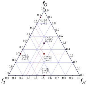
A ternary plot or simplex is a three-variable diagram on which each point in the plot represents the proportions between the three considered variables, and is obtained asfx= _x+y+zx ,fy = _x+y+zy andfz= _x+y+zz . In our case, each axis corresponds

to the fractional values of the structural patterns we analyze: the bottom-left vertex represents purely in-block nested networks (fractional values:fN =fQ= 0,fI = 1), the bottom-right represents networks that are purely nested (fN = 1,fQ=fI= 0), and the top vertex those networks that are purely modular (fN =fI= 0,fQ = 1). This representation is convenient to explore

which network structural configurations map onto which region on the ternary plot.

0.0 0.1 0.2 0.3 0.4 0.5 0.6 0.7 0.8 0.9 1.0 1.0 0.9 0.8 0.7 0.6 0.5 0.4 0.3 0.2 0.1 0.0 0.0 0.1 0.2 0.3 0.4 0.5 0.6 0.7 0.8 0.9 1.0  ≈ 0.5;  ≈ 0.5; Q ≈ 0.  ≈ 0.0;  ≈ 0.66; Q ≈ 0.3  ≈ 0.33;  ≈ 0.33; Q ≈ 0.33  ≈ 0.25;  ≈ 0.25; Q ≈ 0.5  ≈ 0.0;  ≈ 0.1; Q ≈ 0.9

f

f

f

FIG. S2: Representation of the three variables in the ternary plot showing exemplar points with different proportions.

III. SUPPLEMENTAL SECTION II: ANALYTIC EXPRESSIONS ALONGF2FOR THE CASES OFB= 1ANDB= 2 This section provides a complementary formulation for two particular cases of the ring of star graphs,Gs. In the main text,

3 andIfor the cases of a single star (B= 1) and two stars connected through their central nodes (B = 2). As stated in the main text, for these two situations, we have to take into account the change in the number of inter-community links and the degree of the generalist nodes.

A. Nestedness 1. A single star graph,B= 1

The computation of the pair overlap for the evaluation of nestedness whenB = 1requires only the following terms: the pair overlap of a generalist node (the center of each star subgraph),g, with the specialist nodesswhich isOgs/ks= 0; and the pair

overlap between all the specialists nodesOss/ks = 1, the degree of the generalist node iskg = NB−1and the null model

correctionshOgsi=kgks/BNB = (NB−1)/BNBandhOssi=ksks/BNB= 1/BNB N = 2 NB(BNB−1) −N_BNB−1 B (NB−1) + 1₋ 1 BNB _(N B−2)(NB−1) 2 = (NB−2)(NB−1) N2 B − 2(NB−1) 2 N2 B(NB−1) , (4)

2. Two star graph,B= 2

For this scenario we have to take into account the change on the degree of the generalist nodekg=NBand additional terms

such as: the pair overlap between the two generalistsOgg/kg, the pair overlap between a generalist with the specialist from the

other communityOgsout/ks, and the pair overlap between a specialist with the specialists from the other communityOssout/ks. Finally, we obtain N = BN 3 B−BNB2 −6NB2 + 8NB−3 BN2 B(BNB−1) (5) B. Modularity 1. A single star graph,B= 1

Starting with the equation for modularity expressed as sum over the communities (Eq. 2 of the main text), we obtain the total number of links in the network and the number of links per community for a single star graphNB−1, and the sum of the degrees

of the nodes in the communitydc= 2(NB−1). Now, we have the maximum modularity forB= 1.

Q=B " (NB−1) (NB−1) − _2(N B−1) 2(NB−1) 2# = 0, (6)

2. Two star graph,B= 2

WhenB = 2the total number of links changes to L = B(NB −1) + 1and the sum of the degrees of the nodes in the

Q=B " (NB−1) B(NB−1) + 1− _2N B−1 2(B(NB−1) + 1) 2# = 2 " (NB−1) 2(NB−1) + 1 − _2N B−1 2(2(NB−1) + 1) 2# = (2NB−2) 2NB−1 − 1 2 , (7) C. In-block nestedness 1. A single star graph,B= 1

Once again, we know that we will have only two contributing terms to our sum; the pair overlap between specialists(s)nodes and the pair overlap of the generalist(g)node with the specialists. Additionally, we know that for this case the degree of the generalist node iskG=NB−1and the rest of the terms are: the number of specialists nodesNs= (NB−1), the null model

correctionshOg,si=kgkg/BNB = (NB−1)/BNB andhOs,si=ksks/BNB = 1/BNB, an the size of the communities is

C=NB. Finally the analytical expression for in-block nestedness whenB= 1reads,

I= 2 NB −(NB−1)/BNB (NB−1) (NB−1) + ₁ −1/BNB (NB−1) (NB−2) (NB−1) 2 = 2 NB −(NB_N−1) B + _(N B−1)(NB−2) 2NB , (8)

2. Two star graph,B= 2

Now, forB = 2we have that the degree of the generalist node iskG=NB. Substituting this term we obtain a new expression

for the in-block nestedness as

I= 2 NB −_N1 B + _(2N B−1)(NB−2) 4NB , (9)

IV. SUPPLEMENTAL FIGURE 3

Figure S3 shows the results with respect to the parameters of the probabilistic network generation model employed to perform the numerical exploration as explained in the main text (Fig 1). The model is described in detail in the Supplemental Section I. Panel (a)-(d) show the results with respect to varying values of the number of blocks (B), shape parameter (ξ), intra-block (p)

and inter-block noise (µ), respectively. The color bar indicates the mean value of the respective parameter in each bin of the simplex.

5

(a) (b) (c) (d)

FIG. S3: Ternary plots representing results for∼2_×105_{networks as in the main text. In this case, color in each bin of the simplex indicates} the average number of blocksB(A); average shape parameterξ(B); average intra-block noisep(C); and finally average inter-block noiseµ

(D).

V. SUPPLEMENTAL FIGURE 4

Figure S4 shows the values ofQplotted against_N, for the all the generated networks employed in the numerical exploration

in the main text (_∼2_×105_{). The corresponding upper and lower bounds were plotted on top. The color bar, in each case,}

indicates the values of the respective parameters of the probabilistic network generation model (number of blocks (B), shape parameter (ξ), intra-block (p) and inter-block noise (µ), respectively).

(a) (b) (c) (d)

FIG. S4: Optimized values ofQplotted againstN, for the generated networks. The values of the corresponding upper and lower bounds were plotted on top (black dots). The color bar indicates the value of the respective parameters of the probabilistic network generation model (number of blocks (B), shape parameter (ξ), intra-block (p) and inter-block noise (µ), respectively).

VI. SUPPLEMENTAL FIGURES 5 AND 6

For the sake of completeness, we have plotted the values of_Iagainst_N (Fig. S5) andQagainst_I(Fig. S6).

Similar to Fig. 3A in the main text, upper and lower bounds forIhave been calculated in Fig. S5, taking actual measurements ofN as a starting point. Remarkably, none of the optimized values ofIviolates such bounds. This is no surprise with respect to lower bounds, sinceIreduces toN whenB= 1, thus the lower bound simply represents the hard limitI=N. But even the upper bounds, which represent an estimation, are in excellent agreement with respect to the optimized values ofI.

On the other hand, the main lesson from Fig. S6 is the fact that, unlikeQand_N, other patterns can coexist, i.e. there is no

FIG. S5: Values ofIobtained after optimization (grey dots), plotted againstN for the generated networks. Upper and lower bounds ofIare plotted in colors. The color bar indicates the network’s size

(a) (b) (c) (d)

FIG. S6: Optimized values ofQplotted against the optimized values ofI, for the generated networks. The color bar indicates the value of the respective parameters of the probabilistic network generation model. Panel (a) show the results with respect to the number of blocks. Panel (b) correspond to the shape parameterξ. Panels (c) and (d) correspond to the noise parameterspandµ, respectively.

[1] A. Sol´e-Ribalta, C. J. Tessone, M. S. Mariani, and J. Borge-Holthoefer. Revealing in-block nestedness: detection and benchmarking.Phys. Rev. E, 97(6), 062302, 2018.