The Adjustable Balance Mortgage:
Reducing the Value of the Put
Brent W. Ambrose, Ph.D.
Institute for Real Estate Studies
Smeal College of Business
The Pennsylvania State University
University Park, PA 16802
(814) 867-0066
[email protected]
and
Richard J. Buttimer, Jr., Ph.D.
Department of Finance
Belk College of Business Administration
The University of North Carolina at Charlotte
9201 University City Boulevard
Charlotte, NC 28223-0001
(704) 687-7695
[email protected]
The Adjustable Balance Mortgage:
Reducing the Value of the Put
ABSTRACT
We propose a new mortgage contract that endogenously captures the risk of house price declines to minimize default risk resulting from changes in the underlying asset value while still retaining contract rates near the cost of a standard fixed-rate mortgage. By reducing the role of the legal system in mitigating house price risk, the new mortgage reduces the negative externalities and social costs arising from defaults. In other words, the new mort-gage minimizes the need to use the legal foreclosure system to deal with the economic risk of house price declines.
JEL Classification: G0, G13, G18, G2, G21, G28, R28
Introduction
Why do borrowers default? Modern option pricing theory shows that the preponderance of defaults are a result of the home price declining to less than the value of the outstanding mortgage. Prior to the development of this theory, however, mortgage default was assumed to result from either a moral failing on the part of the borrower or from cash flow problems that prevented the borrower from repaying the debt. As neither cause could be hedged, the mortgage contract developed out of the legal traditions of contract enforcement in order to minimize borrower default risk. In the U.S., these legal traditions center on the use of foreclosure laws to take the underlying property from a borrower in default in order to satisfy
the lender’s loss on the defaulted debt.1
Periods of economic turmoil, however, illustrate with stark clarity the inherent inefficiencies of financial contracts designed for previous eras and provide the impetus for financial inno-vation and reform. For example, prior to the Great Depression, the typical U.S. mortgage was a 5-year, interest-only note. The non-amortizing feature of these loans exposed lenders to significant default risk, which was confirmed when housing prices plummeted following
the stock market crash of 1929, leading to massive mortgage foreclosures during the 1930s.2
As part of the New Deal legislation enacted to respond to the financial crisis of the Great Depression, the new Federal Housing Administration (FHA) led the efforts to create the 30-year, fully amortizing fixed-rate mortgage (FRM) that became the standard instrument
for the next 75-years.3
The current mortgage default crisis resulting from the housing bubble of 2004 to 2006 demon-strates the dramatic deadweight costs associated with using the legal system (i.e. foreclosure) to minimize borrower defaults, and suggests the need for a new mortgage that will eliminate or significantly reduce the risks associated with volatile property markets. The financial
cri-sis also demonstrates a fundamental flaw in the current housing finance system: the threat of foreclosure is not sufficient to prevent widespread default when house prices fall significantly. Thus, we propose a new “adjustable balance” mortgage contract that endogenously captures the risk of house price declines to minimize default risk resulting from changes in the under-lying asset value while still retaining contract rates near the cost of a standard mortgage. By reducing the role of the legal system, the new mortgage reduces the negative externalities and social costs arising from defaults resulting from house price risk. In other words, the new mortgage minimizes the need to use the legal system to deal with the economic risk of house price declines.
Our analysis proceeds as follows: In Section , we describe the economic and legal treatment of mortgage default. Section then presents the new Adjustable Balance Mortgage (ABM) concept. Section presents a formal model for pricing this mortgage. Our pricing model allows for fully endogenous borrower prepayment and default, and thus allows us to solve for the equilibrium contract interest rate across products. Thus, we are able to explicitly price the automatic modification features of this product relative to the traditional fixed-rate mortgage (FRM) contract. Section presents the numerical analysis of the ABM and FRM contracts. Section follows with a discussion of the impact of incorporating default transaction costs into the analysis. Finally, Section concludes.
Economic Incentives vs. Legal Costs of Default
Economic theory shows that all mortgages have two primary sources of uncertainty: interest rates and house prices. The contractual treatment of these risks, however, is asymmetric. The mortgage contract explicitly addresses interest rate risk, but it contains no similar
treatment of housing price risk. As a result, defaults must be litigated as opposed to being resolved contractually. This litigation is expensive for both parties and imposes externalities and deadweight losses on society.
To illustrate this disparity in treatment of risk, consider first interest rate risk. The right of the borrower to prepay is explicitly allowed in most residential contracts and explicitly controlled in most commercial mortgages. Furthermore, borrowers can elect to take interest rate risk through the adjustable-rate mortgage (ARM), or pay the lender (through higher contract rates) to bear this risk with a fixed-rate mortgage (FRM). Lenders can elect to issue FRMs or ARMs depending upon their risk preferences. Competitive forces in the lending market have resulted in a wide variety of mortgage alternatives (with different adjusting periods, interest rate caps and floors, and payment options) that allow lenders and borrowers to contract on the degree of interest rate risk each side wishes to bear.
The market, however, has not evolved similar flexibility with respect to housing price risk,
as traditional mortgage contracts are silent with respect to this risk.4 Indeed, from a purely
contractual standpoint the borrower is the one that bears all of the housing price risk. One of the principal insights gained from the application of option pricing theory to mortgage contracts, however, is that the borrower implicitly has the ability to hedge exposure to house price risk through default: if house prices fall enough the borrower can simply default and
“sell” the house to the bank.5,6 Thus, the reality is that under the current system borrowers
and lenders explicitly share the risk of a decline in housing prices with lenders taking the
risk of borrower default.7
The net effect of the current legal framework surrounding the mortgage system is that lenders actually bear, albeit indirectly, house price risk. This creates two problems for lender. First, they must utilize the courts in order to resolve a default – a costly process both in terms of money and time. Second, because the exposure is indirect it is very difficult to hedge
this risk using any type of financial instrument. Although the relatively new futures market for house prices offers a limited ability to hedge housing markets in certain cities, the S&P Case-Shiller index-based derivatives are very costly to use as hedging instruments because of
basis risk.8 This basis risk stems from the effect of the interaction of house prices and interest
rates on the options to default and prepay. In fact, the low trading volume associated with the S&P Case-Shiller indexes suggests that market participants do not find these contracts
sufficient to hedge default risk on the traditional mortgage contracts.9
As a result of the difficulty in hedging default risk, mortgage contracts and the legal tradition
surrounding them were designed to minimize the potential for borrower default.10 The legal
system imposes deadweight costs on both the borrower and the lender in order to provide incentives for both parties to avoid default. Indeed, if one assumes that mortgage contracts were designed to deter a moral problem, then it would make sense to make default as costly
as possible.11 In fact, the legal foreclosure process does exactly this. For example, Hatcher
(2006) reports that a leading mortgage lender estimates that foreclosures cost over $50,000 per incident. Earlier analysis by Ambrose and Capone (1996) using data from the early 1990s noted that typical direct costs to the lender associated with foreclosure (representing legal and sales expenses) were approximately 11 percent of the initial mortgage loan amount, in addition to the unrecovered loss on the loan balance. Finally, borrowers who default face higher credit costs in the future while lenders face uncertain costs over holding and selling the collateral property.
Instead of focusing on the “moral” aspect of the borrower’s ability to pay, we propose a new mortgage contract that effectively minimizes the borrower’s incentive resulting from declining house prices to exercise the embedded put option. Our new mortgage automatically resets the principal balance at various dates to the minimum of the originally scheduled balance or the value of the house, reducing the borrower’s incentive to default if the house value
declines.12 We refer to this contract as the Adjustable Balance Mortgage (ABM).13
The Adjustable Balance Mortgage (ABM)
At origination, the ABM is like a fixed-rate mortgage in that it has a fixed contract rate, maturity term, and is fully amortizing. At fixed, pre-set intervals, the lender and the bor-rower determine the value of the house. If the house value is lower than the then originally scheduled balance for that date, the loan balance is set equal to the house value, and the monthly payment is re-calculated based on this new value. If the house retains its initial value or increases in value, then the loan balance and payments remain unchanged just as in a standard fixed rate mortgage.
Obviously, the process for determining the mortgage collateral value is critical to the success of the ABM. We envision that the house value will be determined through a repeat-sales index, or some other form of an area-wide index. We recognize that this approach suffers from basis risk, but we believe that it offers the fewest drawbacks possible and the most
benefits over other alternatives.14 First, the use of an area house price index eliminates the
need for costly (and time consuming) independent appraisals. Second, and perhaps more importantly, adjusting the collateral value to an area house price index (e.g. city or regional index) eliminates the risk of moral hazard created by adjusting the mortgage balance to the specific collateralized property. If the mortgage balance were tied explicitly to the value of the house, then the borrower would have an incentive and the ability to intentionally reduce the house value through neglect. Third, from the lenders’ perspective the house price
changes reflected in an index mirror their systematic risk exposure to a city or region.15
the effects of basis risk and how the ABM contract mitigates it, consider the following two scenarios: First, the house value increases but the index either declines or stays flat; and second, the house value decreases but the index increases. In the first case, the mortgage is reset to a lower value when the asset value did not fall, and thus the burden of the basis risk is born by the lender. The lender, however, would presumably have a portfolio of these loans and, assuming that the index correctly captures the general area price movement, then on average the portfolio would be priced accurately. Furthermore, this form of basis risk is a
standard concern in portfolio hedging.16 Thus, even though the lender bears basis risk, they
could greatly mitigate it through both portfolio effects and through hedging with derivatives.
The second instance of basis risk works to the disadvantage of the borrower, although we argue that the design of the ABM minimizes this effect. Under this scenario the house value declines but the index increases or stays flat. In this case the balance should be reduced, but would not be. Although this denies the borrower some of the benefit from the ABM, their balance does not go up as would be the case with other alternative models that have been proposed and are discussed below. Further, the borrower is no worse off than they would be under a standard fixed rate mortgage, and, in fact, would still have the option to default. It would also be possible to envision an appeals process, something similar to property tax appeals, whereby a borrower who felt that changes in the index materially misrepresented changes in the value of the home could pay to have the house independently appraised.
An example
To illustrate the adjustment process, assume that the house price index declined from origi-nation to the first adjustment date and consider the following three scenarios at the second adjustment date: an upward movement in house prices, no change in house prices, or a
further decline in house prices. In the first case, the house value index increases between the first and the second adjustment dates. Thus, the balance is increased to the minimum of the new house value or the originally scheduled balance at the second adjustment date. As a result, the monthly payment goes up, but it does not exceed the mortgage payment specified at origination.
In the second case, the house value is exactly the same as at the first adjustment date. The balance is set to the minimum of the scheduled balance for that month or the house value. If the original amortization has reached the point where the balance would be less than the house value, then, of course, the payment is just the original payment. If we have not reached that point, however, then the balance is set to the house value and the payment is recalculated - this means that from the first reset to the second reset date the balance would remain constant (actually, it would amortize each month, but then reset to the old value because the house valued remained constant.)
Finally, in case three, the house value declines between the first and second adjustment dates. Thus, the new balance is the new house price and the monthly payment is adjusted lower accordingly.
The ABM results in an explicit risk-sharing between the borrower and lender with respect to house prices. Before the loan balance is reset, the borrower will have lost whatever initial equity they had in the property, plus any equity that they would have built-up through the amortization process. Should the house price fall below the balance triggering a reset, and the house value then subsequently rises, the lender recovers their lost value first. In addition, if the house value rises above the originally scheduled balance on a reset date, then the owner begins to recover their equity as well. Note that the provision for the borrower to recover equity provides an economic incentive for the borrower to maintain the property even in the face of substantial price declines. Standard mortgages lack this economic incentive and
evidence clearly shows that borrowers fail to maintain their properties when anticipating
future default.17
Comparison of the ABM to other alternative contracts
Our adjustable balance mortgage is similar in spirit to a number of recently proposed al-ternative mortgages contracts, including the Danish “mark-to-market” mortgage, the “buy your own mortgage” (BYOM) innovation proposed by Hancock and Passmore (2008), and the “continuous workout mortgage” (CWM) proposed by Shiller (2009). Each of these al-ternatives attempts to limit borrower default.
As Svenstrup and Willeman (2006) point out, the Danish mortgage gives the borrower the option to prepay at the mortgage market value rather than at par (as in the U.S.). During periods when market interest rates are higher than the contract rate, the mortgage market value is less than the loan balance (par value). Thus, the Danish mortgage might reduce the incentive to default if the house value is less than the mortgage balance and the mortgage market value is less than the house value, as the borrower has the option to prepay at the lower market value. However, in order to realize this gain, the borrower must incur significant transaction costs (either in the form of mortgage origination fees if they refinance or through sales expenses and taxes associated with sale and relocation.)
Furthermore, while interest rates do play a part in the decision to default, as we show below they are not the primary cause of defaults. The primary cause of default is a decline in the value of the underlying collateral and the Danish mortgage does not address this issue. For example, consider the scenario where the value of the underlying property declined by 25%, but market interest rates remained at the level at loan origination. As a result, the
borrower would have to make a prepayment that was larger than the value of the collateral. Thus, to the extent that property value declines are significantly greater than reductions in the mortgage value due to increases in mortgage interest rates, the borrower will retain an
incentive to engage in strategic default.18
Finally, even if mortgage interest rates increase sufficiently to offset a decline in the house price, and thus transform what would have been a default event into a prepayment event, the Danish mortgage still relies upon sufficient market liquidity for the borrower to be able to secure a new mortgage. Clearly during the recent mortgage liquidity crisis in the U.S., this was not always the case.
The ABM, in contrast, does not suffer from these problems. First, the balance of the loan, and hence the prepayment amount required to pay it off, explicitly incorporates the value of the underlying collateral. Second, the adjustments are endogenous to the loan contract, and unlike the Danish mortgage, do not rely upon the liquidity of the mortgage market to reduce the default incentive.
Borrowing from the Danish concept, Hancock and Passmore (2008) propose a mortgage that gives the borrower the right to pay the lender the proceeds from the house sale rather than the par value, in essence giving the borrower insurance against declines in the house value. We see two difficulties with the BYOM system. First, in order to realize the benefits of the plan, the borrower has to sell the house, as the mortgage payment and balance are never adjusted downward if the house price declines. These sales are costly, and once again rely upon liquidity in the housing market. Second, and more importantly, the BYOM exposes the lender to significant moral hazard as the borrower has control over the underlying asset price. Indeed, the borrower would have an extremely strong incentive to accept side payments that were not formally part of the sales contract in order to reduce the contracted sales price of the house. One can even envision a scenario where two unscrupulous BYOM borrowers
would agree to “sell” their houses to each other at low prices, pay off the BYOM mortgages at these lower prices, and then later on sell their original houses back to each other; that is, in essence they would enter into a repurchase agreement with the intent of defrauding the BYOM lender. Given borrower behavior during the subprime bubble, it is clear that moral hazard is a significant issue, and the BYOM mortgage lender would have large exposure to it.
While one could envision a system of auditing sales contracts under the BYOM plan, this would be a costly and intrusive process. The ABM in contrast does not expose the lender to this type of moral hazard risk. Further, because the adjustments are endogenous to the mortgage, the borrower does not have to sell their house to reap the benefits of the mortgage resets.
The continuous workout mortgage (CWM) advocated by Shiller (2009) is similar to the ad-justable balance mortgage in that the mortgage balance is automatically adjusted to changes in a neighborhood (or area) house price index. The continuous workout mortgage advocated by Shiller (2008) originally proposed to adjust the mortgage terms based on fluctuations in borrower income. Shiller (2009) suggested a variation that adjusts the mortgage balance based on changes in an area house price index but deferred development of the contract details. However, unlike the ABM, the CWM concept is designed to keep the borrower’s equity constant. The CWM decreases the mortgage balance when home prices decline and increases the balance when home prices rise. Shiller (2009) does not explicitly describe how these adjustments would work, and in particular, he leaves open the issue of whether there would be limits to increases in the balance of the mortgage if the house price index rose.
Although Shiller does not discuss the upward adjustment process, this is critical to the design of the contract. At first blush it would appear to be reasonable to assume that if there were no limits on the downward adjustment when the index fell then there should be no limits
on the upward adjustments either. Unlimited upward adjustments, however, create at least three significant problems.
First, unlimited upward adjustments have the potential to create a housing affordability problem. If house prices increase more rapidly than wages, then borrowers that face budget constraints may find that they cannot make the increased mortgage payment. This would be especially problematic in areas where house prices increased very rapidly, as happened in several places in the U.S. during the 2000’s. While it would be true that the borrower would be wealthier because their house would be worth commensurately more, they would have no ability to monetize that increased wealth except by selling the home.
Second, in essence unlimited upward adjustments grant the lender an equity position in the house. Thus, the mortgage balance increases if the home prices rise, limiting the capital accumulation feature of home ownership that is often considered one of the major benefits of home ownership. This may create a disincentive for the borrower to improve or even maintain the home. It would also encourage a borrower to try to time the sale or refinancing of a home to avoid sales when home prices are increasing.
Third, the unlimited upward adjustments would expose the borrower to enhanced basis risk. If the index increased while the individual house price declined, then the borrower would have a very strong incentive to default. Under this scenario, a borrower would find their balance and payments increasing even though their actual house value was declining.
The ABM balance adjustment process eliminates or significantly mitigates all of these issues. It is designed such that the monthly payment never exceeds the original payment amount, thus eliminating the risk that the borrower would face an affordability problem caused by an increase in the home price index. Second, the ABM balance never exceeds the original
As a result, the ABM preserves the borrower incentive to maintain and improve the home. Even if the home price declines significantly, such that the borrower effectively has a 100% LTV mortgage, once house prices rose to their original level, the borrower would begin to accumulate equity again, creating an incentive for the borrower to maintain the home. Finally, although the ABM does suffer from some basis risk, as previously discussed, this basis risk is significantly smaller and the consequences to the borrower are much less onerous than that associated with unlimited adjustments. Under the ABM, the basis risk may result in the borrower not getting a balance and payment reduction to which they should be entitled, but under unlimited upward adjustments their balance and payment would actually increase.
Recently, Piskorski and Tchistyi (2010) develop a theoretical model of an “optimal” mortgage contract that attempts to explain the recent growth in the use of option adjustable-rate mortgages and interest-only mortgages. Their model extends the framework developed in the finance literature on dynamic optimal contract design by introducing a stochastic interest
rate.20 However, their model focuses on volatility in borrower income with respect to an
exogenous boundary as the condition for default and explicitly ignores the role of asset price declines in motivating strategic default. In contrast, our development of the ABM focuses on reducing or eliminating the endogenous strategic default condition inherent in all mortgage contracts.
In addition to innovative mortgage products, a number of commercial firms have attempted to introduce option contracts on house appreciation that would provide some protection to the borrower from a decline in house prices. For example, EquityRock has attempted to create a real estate option contract that provides the homeowner with the ability to sell a
portion of the future equity appreciation in exchange for a guaranteed payout.21 Although
this contract does provide the homeowner with some insurance protection in the event of house price declines (though the guaranteed payout), the contract does not eliminate the
incentive for borrowers to engage in strategic default if asset values decline.
A Formal Contingent Claims Model of the ABM
As is customary in the mortgage pricing literature, we develop a model of the ABM by utilizing the insights from Black and Scholes (1973) to note that in a perfect capital market the present value of a contingent claim (such as a mortgage contract) is:
𝑉(𝑟, 𝐻, 𝑇) =𝐸
[
𝑒−∫0𝑇𝑟(𝑡)𝑑𝑡𝑉(𝑟, 𝐻, 𝑇)] (1)
where 𝑉(𝑟, 𝐻, 𝑇) is the terminal value of the mortgage contract expiring at 𝑇, and𝐸 is the
risk-neutral expectations operator. The model contains two sources of uncertainty, interest rates (𝑟) and house prices (𝐻). We assume interest rates follow the Cox, Ingersoll, and Ross (1985) process:
𝑑(𝑟) = 𝛾(𝜃−𝑟)𝑑𝑡+𝜎𝑟
√
𝑟𝑑𝑧𝑟 (2)
where𝜃 is the steady state mean rate,𝛾 is the speed of adjustment factor,𝜎𝑟 is the volatility
of interest rates, and 𝑑𝑧𝑟 is a standard Wiener process.
For the second risk factor, we assume the physical house price follows the standard stochastic process,
𝑑𝐻
where 𝛼 is the total return to housing, 𝑠 is the service flow, 𝜎𝐻 is the volatility of housing
returns, and 𝑑𝑧𝐻 is a Wiener process. Assuming the correlation coefficient between 𝑑𝑧𝐻 and
𝑑𝑧𝑟 is 𝜌, and substituting the risk-neutral drift rate 𝑟 for 𝛼 in equation (3), then equation
(1) is the solution to the following partial differential equation (PDE)
1 2𝐻 2𝜎2 𝐻 ∂2𝑋 ∂𝐻2 +𝜌𝐻 √ 𝑟𝜎𝐻𝜎𝑟 ∂2𝑋 ∂𝐻∂𝑟 + 1 2𝑟𝜎 2 𝑟 ∂2𝑋 ∂𝑟2 +𝛾(𝜃−𝑟) ∂𝑋 ∂𝑟 + (𝑟−𝑠)𝐻 ∂𝑋 ∂𝐻 + ∂𝑋 ∂𝑡 −𝑟𝑋 = 0 (4)
solved backwards through time.
Clearly the ABM is a highly-path dependent mortgage, and as such does not have a closed-form solution. As a result, we use a numerical method based on Nelson and Ramaswamy (1990) to value the mortgage and to solve for equilibrium contract rates. This method
doubly transforms the two state variables, 𝑟 and 𝐻, to allow for a simpler two-dimensional
binomial-model.22 We model the ABM and a standard fixed-rate mortgage (FRM) within
this bivariate-binomial lattice.
Boundary Conditions at Maturity (𝑇
)
Given that we can model the evolution of𝑟and𝐻, we must define the appropriate boundary
conditions for the FRM and the ABM. Since the model uses backwards-induction, we begin with the boundary conditions at the terminal time. Consider first the terminal boundary
conditions for the FRM with an annual contract rate 𝑟𝑐 and where the monthly mortgage
payment (𝑃 𝑀𝑇𝑡) is given by:
𝑃 𝑀𝑇𝑡=B0∗ [ 𝑟𝑐/12 1− 1 (1+𝑟𝑐/12)𝑡 ] , (5)
for 𝑡 = 1 to𝑇 and where 𝐵0 is the mortgage balance at origination. At termination, the
present value of the promised payments, 𝐴𝑇, is given as:
𝐴𝑇 =𝑃 𝑀 𝑇𝑇. (6)
Furthermore, the values of default, prepayment, and the mortgage are given as:
𝐷𝑇 = 𝑚𝑎𝑥[0, 𝑃 𝑀𝑇𝑇 −𝐻𝑇] (7)
𝐶𝑇 = 0 (8)
𝑉𝑇 = 𝐴𝑇 −𝐶𝑇 −𝐷𝑇. (9)
The terminal boundary conditions for the ABM are similar since the borrower only faces one decision at the terminal time step, make the final payment or default. However, the ABM is operationally much more complex because the payment amount is not fixed, but rather is
conditional upon the balance remaining after the last reset date, denoted as 𝑇 −𝑇𝑅, where
𝑇𝑅 is the number of months following the last reset date.
At time 𝑇, we do not know with certainty the balance at the last reset date because we do
not know the path of house values through time. We do, however, know the upper bound, which is the originally scheduled balance for that reset date. Because of the structure of the bivariate binomial lattice, we also know that only a finite number of potential mortgage
balances exist as of that reset date.23 From the potential balances at 𝑇 −𝑇
𝑅, we then
determine the finite number of potential balances that exist at termination 𝑇.
terminal values for default, prepayment, the promised mortgage payment, and the value of the mortgage conditional upon the payment value. Formally, we make the ABM payment
conditional upon the balance at the previous resetting date,𝐵𝑙𝑎𝑠𝑡.24 This is given by:
𝑃 𝑀𝑇𝑇∣𝐵𝑙𝑎𝑠𝑡 =Blast ∗ [ 𝑟∗ 𝑐/12 1− 1 (1+𝑟∗ 𝑐/12)𝑇𝑅 ] , (10) where𝑟∗
𝑐 represents the ABM contract interest rate set at origination. The boundary
condi-tions for the ABM are:
𝐴𝑇∣𝐵𝑙𝑎𝑠𝑡 = 𝑃 𝑀𝑇𝑇∣𝐵𝑙𝑎𝑠𝑡 (11)
𝐷𝑇∣𝐵𝑙𝑎𝑠𝑡 = 𝑚𝑎𝑥[0, 𝑃 𝑀𝑇𝑇∣𝐵𝑙𝑎𝑠𝑡−𝐻𝑇] (12)
𝐶𝑇∣𝐵𝑙𝑎𝑠𝑡 = 0 (13)
𝑉𝑇∣𝐵𝑙𝑎𝑠𝑡 = 𝐴𝑇∣𝐵𝑙𝑎𝑠𝑡−𝐶𝑇∣𝐵𝑙𝑎𝑠𝑡 −𝐷𝑇∣𝐵𝑙𝑎𝑠𝑡. (14)
As we work backwards in time we eventually get to time 𝑇 −𝑇𝑅 at which point we discard
the extraneous values. Of course, the actual balance at time 𝑇 −𝑇𝑅 is itself a function of
the balance at time𝑇 −2∗𝑇𝑅. However, the uncertainty does partially resolve at each reset
date, providing sufficient resolution of the uncertainty to allow us to work our way back to time 0, at which point all uncertainty resolves. The uncertainty applies to all calculations that are dependent upon the balance of the loan, including payments, the default option, and the prepayment option.
Boundary Conditions Prior to Maturity (𝑡 < 𝑇
)
For both the FRM and the ABM at payment dates other than the terminal date, the bor-rower chooses between one of three actions. First, the borbor-rower can make the schedule payment, thus continuing the mortgage. Second, the borrower can terminate the mortgage via prepayment. Third, the borrower can terminate the mortgage through default. For the FRM, the present value of the future promised payments is:
𝐴𝑡=𝑃 𝑀𝑇𝑡+
𝐸[𝐴𝑡+1]
(1 +𝑟𝑡)
, (15)
where𝐸[𝐴𝑡+1] is the expected value of𝐴at the next time step.25 The payoff to continuation
is:
𝑉𝑡 =𝐴𝑡−𝐶𝑡+−𝐷+𝑡 , (16)
where𝐶+
𝑡 equals the expected present value of the future prepayment option (𝐶𝑡+=𝐸[𝐶𝑡+1]/(1+
𝑟𝑡)), and𝐷+𝑡 is the expected present value of the future default option (𝐷+𝑡 =𝐸[𝐷𝑡+1]/(1 +
𝑟𝑡)).
Recognizing that the borrower selects one of three choices, then the value of prepayment
(𝐶∗ 𝑡) is given as: 𝐶∗ 𝑡 = ⎧ ⎨ ⎩ 𝐶𝑡+= 𝐸[𝐶𝑡+1]
(1+𝑟𝑡) if the borrower makes the scheduled payment
𝐴𝑡−𝐵𝑡 if the borrower prepays
0 if the borrower defaults
Similarly, the value of default (𝐷∗ 𝑡) is given as: 𝐷∗ 𝑡 = ⎧ ⎨ ⎩ 𝐷+
𝑡 = 𝐸(1+[𝐷𝑡𝑟+1𝑡)] if the borrower makes the scheduled payment
𝐴𝑡−𝐻𝑡 if the borrower defaults
0 if the borrower prepays
(18)
Thus, for example, if the borrower prepays then the lender only receives the balance from the loan:
𝐴𝑡−𝐶𝑡∗−𝐷∗𝑡 =𝐴𝑡−(𝐴𝑡−𝐵𝑡)−0 = 𝐵𝑡 (19)
or if the borrower defaults then the lender receives the collateral:
𝐴𝑡−𝐶𝑡∗−𝐷∗𝑡 =𝐴𝑡−0−(𝐴𝑡−𝐻𝑡) = 𝐻𝑡 (20)
Therefore, the lender receives𝐴𝑡−𝐶𝑡+−𝐷𝑡+ if the borrower makes the scheduled payment,
the outstanding balance (𝐵𝑡) if the borrower prepays, or the house value (𝐻𝑡) if the borrower
defaults. The borrower will select the option that maximizes their wealth, or that equiva-lently minimizes the wealth of the lender. As a result, the value of loan to the lender is given as:
For the ABM, the borrower applies the same logic. That is, the borrower minimizes the wealth of the lender in order to maximize their wealth. The difference is that all of the equations that are dependent upon the balance of the loan at the last reset date must be noted as being conditional values. Thus,
𝐴𝑡∣𝐵𝑙𝑎𝑠𝑡 =𝑃 𝑀𝑇𝑡∣𝐵𝑙𝑎𝑠𝑡+
𝐸[𝐴𝑡+1∣𝐵𝑙𝑎𝑠𝑡]
(1 +𝑟𝑟)
(22)
is the present value of the promised stream of payments, conditional on the balance at the
last resetting date (𝐵𝑙𝑎𝑠𝑡). The value of continuation therefore is:
𝑉𝑡∣𝐵𝑙𝑎𝑠𝑡 =𝐴𝑡∣𝐵𝑙𝑎𝑠𝑡 −𝐶
+
𝑡∣𝐵𝑙𝑎𝑠𝑡 −𝐷
+
𝑡∣𝐵𝑙𝑎𝑠𝑡, (23)
where the conditional values 𝐶+
𝑡∣𝐵𝑙𝑎𝑠𝑡 and 𝐷
+
𝑡∣𝐵𝑙𝑎𝑠𝑡 are still the expected present value of the
prepayment and default options in the future, conditional upon the balance at the last reset date.
As before, the values of prepayment and default are given as:
𝐶∗ 𝑡∣𝐵𝑙𝑎𝑠𝑡 = ⎧ ⎨ ⎩ 𝐶𝑡+∣𝐵𝑙𝑎𝑠𝑡 = 𝐸[𝐶𝑡+1∣𝐵𝑙𝑎𝑠𝑡]
(1+𝑟𝑡) if the borrower makes the scheduled payment
𝐴𝑡∣𝐵𝑙𝑎𝑠𝑡−𝐵𝑡∣𝐵𝑙𝑎𝑠𝑡 if the borrower prepays
0 if the borrower defaults
and 𝐷∗𝑡∣𝐵𝑙𝑎𝑠𝑡 = ⎧ ⎨ ⎩ 𝐷+ 𝑡∣𝐵𝑙𝑎𝑠𝑡 = 𝐸[𝐷𝑡+1∣𝐵𝑙𝑎𝑠𝑡]
(1+𝑟𝑡) if the borrower makes the scheduled payment
𝐴𝑡∣𝐵𝑙𝑎𝑠𝑡−𝐻𝑡∣𝐵𝑙𝑎𝑠𝑡 if the borrower defaults
0 if the borrower prepays
(25)
Finally, from the lender’s perspective, the value of the loan to the lender is:
𝑉𝑡∣𝐵𝑙𝑎𝑠𝑡 =𝑚𝑖𝑛(𝐴𝑡∣𝐵𝑙𝑎𝑠𝑡−𝐶 + 𝑡∣𝐵𝑙𝑎𝑠𝑡−𝐷 + 𝑡∣𝐵𝑙𝑎𝑠𝑡, 𝐵𝑡∣𝐵𝑙𝑎𝑠𝑡, 𝐻𝑡)≡𝐴𝑡∣𝐵𝑙𝑎𝑠𝑡 −𝐶 ∗ 𝑡∣𝐵𝑙𝑎𝑠𝑡−𝐷 ∗ 𝑡∣𝐵𝑙𝑎𝑠𝑡. (26)
We also note that at any interior point other than a payment due-date, the borrower does not have to take any action should they elect to default. Their default decision will only become apparent at the next payment due-date. As a result, at the non-payment due dates, the boundary conditions do not consider the case of immediate default.
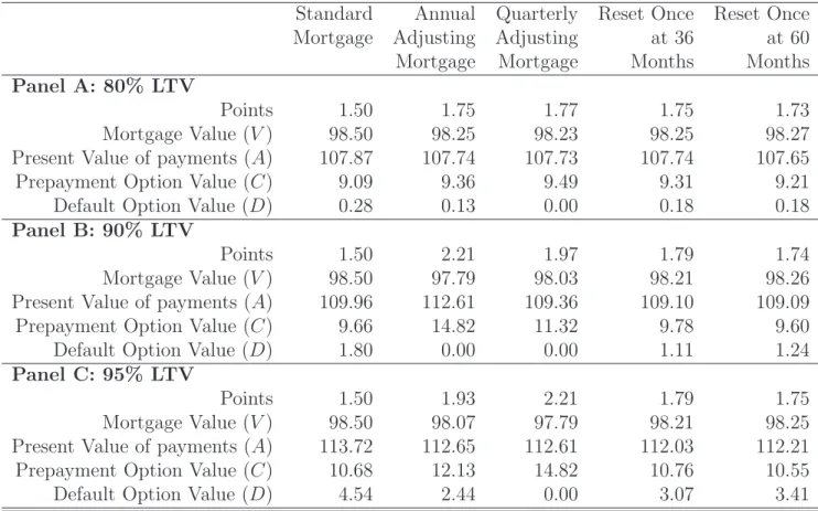
Numerical Analysis
As mentioned above, the path dependency inherent in the ABM precludes a closed form solution and thus we use numerical analysis to solve the equilibrium contract rates and option values. Table 1 summarizes the input parameters used in the numerical analysis. These parameter values are generally consistent with the input parameters used in the literature. We begin the analysis by presenting in Table 2 results showing the equilibrium contract for each mortgage type (FRM and multiple reset-option ABMs) under three common loan-to-value ratio assumptions (80%, 90%, and 95%.) In order to highlight the costs associated
with the ABM, we present four alternative versions. First, we present an annual adjusting contract (the balance is adjusted annually at the mortgage origination anniversary). Second, we demonstrate the impact of more frequent adjustments by pricing a quarterly adjusting contract. Third, we show the pricing for two contracts that reset only once during the mortgage life (at month 36 and month 60). Obviously, many other adjustment date variations
are possible and the alternatives shown in Table 2 are representative.26
The results in each Panel in Table 2 are in equilibrium. That is, we solved for the contract
rate for each mortgage which equates the value of the mortgage (𝑉) with the cash received
at time origination. We assume that the borrower pays 1.5 points at origination and thus the equilibrium “par” value of the mortgage is $98.50. We also present the equilibrium origination values for the present value of the payments (𝐴), the value of the borrower’s prepayment option (𝐶), and the value of the default option (𝐷).
We note that two major results or implications come from Table 2. First, the equilibrium contract rates for the ABM variants are typically 25 to 40 basis points higher than for the standard FRM. For example, in Panel C (the 95% LTV assumption), we note that the equilibrium FRM contract rate is 6.22% while the annual ABM and quarterly ABM have equilibrium contract rates of 6.46 percent and 6.64%, respectively. Thus, the quarterly ABM has an equilibrium contract rate that is 42 basis points greater than the standard FRM contract. In contrast, the premium required for the quarterly ABM under the 80% LTV assumption (Panel A) is only 13 basis points and the premium under the 90% LTV case (Panel B) is 23 basis points. Intuitively, as the LTV increases, the borrower’s initial equity position declines and the probability of the collateral value falling below the mortgage balance increases. As a result, the ABM is more valuable to the borrower for higher LTV contracts and hence the equilibrium contract rate premium increases to compensate the lender for bearing the additional house price risk.
Since the ABM is designed to shift house price risk from the borrower to the lender, Table 2 shows that the ABM dramatically reduces the financial value of the default option, as expected. For example, the annual ABM reduces the value of default by approximately 36% (from 4.54 to 2.9 in the 95% LTV case) while the examples with one-time adjustments at months 36 and 60 only reduce the default value by about 19% and 25%, respectively. How-ever, moving from the annual adjustment to a quarterly adjustment completely eliminates the financial (or rational) incentive for default. Thus, the quarterly ABM is more effective at reducing the value of (i.e. future economic incentive for) default than any of the others.
The second major result evident in Table 2 is that the value of the prepayment option goes up substantially for the ABM contracts. However, the prepayment option value increase is not due to the increase in the equilibrium contract rate, but rather because of the fact that default is no longer a competing source of termination. Although the equilibrium contract rate is higher for the ABM mortgages than for the FRM mortgage, the difference across contract rates is not large. Thus, the factor driving the increase in prepayment is the fact that under the ABM, the borrower does not have the competing risk of default. As a result, borrowers will prepay more rapidly. Furthermore, faster expected prepayment under the ABM is good news from a lender’s hedging standpoint since prepayments will be more tightly tied to interest rate changes.
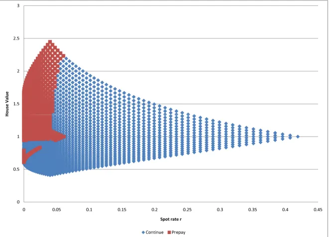
To see the effect on prepayment, consider Figures 1 and 2 that show the borrower’s default, prepayment, and continue regions in state space (house price and interest rate) 36 months
after origination for the standard FRM and quarterly ABM, respectively.27 In essence, the
state space figures show the interaction of house prices and interest rates on the borrower’s decision to continue or terminate the mortgage. For example, the green region in Figure 1 shows the default region for a borrower in a standard FRM at month 36. As expected, default is optimal when house prices have declined (less than 1.0) and spot interest rates are
relatively low (less than 15 percent). The red region reveals the combination of house prices and interest rates where the borrower would optimally prepay the mortgage at month 36 and the blue region represents the combinations of house prices and interest rates where the
borrower would find it optimal to make the next payment.28 In comparison, Figure 2 shows
the borrower’s termination regions at month 36 for the quarterly ABM. Consistent with the results presented in Table 2, the green default region is not present in Figure 2 indicating that default is not an optimal decision for the borrower. However, Figure 2 does show the increase in the value of prepayment as certain regions of the state space where house prices and interest rates are low are dominated by prepayment.
As noted above, the equilibrium contract rates for the various ABM contracts are approxi-mately 25 to 40 basis points from the FRM base case. Thus, we consider whether the increase in the equilibrium contract rate is low enough to induce borrowers to prefer the ABM con-tract over the standard FRM concon-tract. In other words, how much would a borrower be willing to pay, in the form of a higher contract interest rate, to eliminate the potential for
future negative equity?29 In order to answer this question, we recognize that, under the
ABM, mortgage insurance would be either unneeded or priced at such a low rate (to cover frictional, non-financial defaults) that the net cost to the borrower might actually be less than under an FRM. Another way of thinking about the issue of contract desirability is to ask, if the lender kept the contract rate fixed at the current FRM rate, how many points would the borrower have to pay for this loan? In Table 3 we answer this question by holding the interest rate constant at the standard FRM contract rate that balances the contract (as-suming the borrowers pays 1.5 points) and varying the total points paid at origination. For example, in Table 3 Panel C (the 95% LTV mortgage), we assume the mortgage interest rate is 6.2170% for all contracts. We see that for the annual adjusting ABM, the borrower would have to pay 42 basis points more in up-front interest (1.93 points versus 1.5 points under the FRM). For the quarterly adjusting contract that eliminates financially induced default, the
borrower would have to pay 71 basis points more than under the standard FRM contract. In contrast, typical private mortgage insurance (PMI) contracts require the payment of 0.5% (50 basis points) of the loan balance each year while the Federal Housing Administration (FHA) charges an up-front fee of 1.5% (150 basis points) of the loan amount plus a monthly fee. Clearly the additional costs associated with the quarterly adjusting ABM are below the standard costs associated with PMI and substantially lower than the costs associated with FHA insurance.
Our model also allows us to consider the impact of uncertainty, as reflected in the volatility assumptions underlying the stochastic state processes, on the default values and equilibrium interest rates. Thus, in table 4 we report the equilibrium contract values corresponding to the standard mortgage, the annual adjusting mortgage, and the quarterly adjusting mortgage
for combinations of house price volatility (𝜎𝐻) and interest rate volatility (𝜎𝑟). Table 4
reports the results assuming loan-to-values ratios at origination of 80%, 90%, and 95% for
the following volatility combinations: [𝜎𝐻 = 𝜎𝑟 = 5%], [𝜎𝐻 = 5%, 𝜎𝑟 = 15%], [𝜎𝐻 =
15%, 𝜎𝑟 = 5%], and [𝜎𝐻 = 𝜎𝑟 = 15%]. As before, we price the mortgages in equilibrium
with a par value of $98.50. Turning to Panel C (LTV=95%), we find several interesting features. Consistent with option pricing theory, increasing the underlying volatility of the state processes increases the value of the embedded options to default and prepay. For
example, looking at the annual adjusting ABM, we see that increasing 𝜎𝑟 by a factor of
three from 5% to 15% (holding 𝜎𝐻 constant at 5%) increases the value of prepayment from
3.15 to 19.75 and the value of default from 0.14 to 0.57, respectively. Interestingly, increasing the house price volatility by a factor of three has an even greater effect on prepayment than
the corresponding increase in interest rate volatility. For example, increasing 𝜎𝐻 from 5% to
15% (holding 𝜎𝑟 constant at 5%) increases the value of prepayment from 3.15 to 22.11 and
Table 4 also highlights the highly complex interaction between prepayment and default depending upon the assumption regarding the state process volatility. For example, consider the results for the standard mortgage contract. Across all LTV assumptions, we see that
increasing the house price volatility (𝜎𝐻) increases the value of the default option. For
example, looking at the 95% LTV case, we see that increasing 𝜎𝐻 from 5% to 15% (holding
𝜎𝑟 constant at 5%) increases the default value from 0.19 to 10.03. However, for the quarterly
ABM, the same increase in 𝜎𝐻 actually causes the value of default to decrease from 0.06 to
0.00. In other words, default become less likely under the quarterly ABM when house price volatility is high.
Default Transaction Costs
Although we find the difference in equilibrium contact rates to be small, that is a matter of subjective opinion. Thus, we now focus on the following question: Do reasonable circum-stances exist where the ABM contract would have a lower contract rate than a standard FRM? If we assume that the lender faces unrecoverable transactions costs associated with default, then the answer is unequivocally affirmative. Lenders do clearly face such costs. For example, consider that lenders normally hire a real estate agent to sell the foreclosed property, at a typical cost of 6% in most parts of the US. In addition, lenders face other costs including insurance, maintenance, property taxes, and/or utilities while the house is being marketed. Based on these costs, some have estimated that transactions cost may exceed
30% of the outstanding loan balance.30 Note that in our context, transaction costs include
only the costs associated with the delinquency and foreclosure process, and not the loss in value from the house itself.
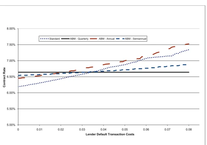
reflect the worst case for the lender when calculating the equilibrium contract rates, we let the lender face default transaction costs but not the borrower. As a result, this creates a wedge in the mortgage value between the borrower and lender at origination. In order to compensate the lender for the anticipated costs if default occurs, all contract rates are higher. As a result, prepayment is higher in general. In order to demonstrate the effect of various levels of transaction costs, we calculated the equilibrium contract rate at every level of lender transaction cost from 0 to 10% (of original house value.) Figure 5 plots the equilibrium contract rates for lender default transaction cost levels for each of the mortgage contracts assuming a 95% LTV. Figure 5 clearly shows that if lender default transaction costs are very low (less than 3% of the original house value), then the standard FRM contract has the lowest contract interest rate. However, at higher levels of lender default costs (greater than 4%), the semiannual and quarterly adjusting ABM contracts have equilibrium contract rates less than the standard fixed-rate mortgage. In other words, under any reasonable assumption of non-recoverable lender default losses, the quarterly adjusting ABM contract would have a lower interest rate to the borrower than the current standard FRM for high LTV mortgages.
The results are less intriguing at an 80% LTV, where our analysis indicates that the FRM always has a lower equilibrium contract rate than the ABM variations. However, this result is largely determined by the fact that default is relatively rare with an 80% LTV mortgage. For example, in Table 2 we saw that the value of default was approximately 28 basis points for the FRM option and 13 basis points for the annual ABM contract. In addition, the defaults, when they do happen, tend to occur later in the life of the mortgage since it takes time for the house value to fall below the mortgage balance in order to trigger an optimal default. As a result, present value discounting effects also come into play. Nevertheless, it is the case that at 80% LTV, the FRM always has a lower equilibrium contract rate than the ABM suggesting that the ABM contract would be preferred by borrowers seeking higher
LTV contracts.
Conclusion
Following the tradition that economic crises often spur financial innovations, we propose a new fixed-rate mortgage contract that mitigates the risks associated with downward move-ments in house prices. Similar to the adjustable-rate mortgage that shifts interest rate risk from the lender to the borrower, our new adjustable balance mortgage (ABM) shifts house price risk from the lender to the borrower. The ABM automatically resets the principal balance at various dates to the minimum of the originally scheduled balance or the value of the house.
Using a standard bivariate-binomial lattice model, we demonstrate numerically that the value of the borrower’s default option declines as the frequency of balance resets increases. Our analysis reveals that the borrower’s default option is effectively eliminated under a quarterly balance adjusting mortgage. Since we solve the contract values in equilibrium, our analysis shows that for a 95% LTV mortgage, the cost to the borrower for the quarterly ABM, in the form of a higher contract interest rate, is 42 basis points relative to the standard fixed-rate contract. However, under any scenario assuming reasonable dead-weight losses to the lender from default, our analysis demonstrates that the ABM has lower contract rates than the standard fixed-rate mortgage when the loan-to-value ratio is above 80%.
As previously mentioned, the interaction of the default and prepayment options in a fixed rate mortgage make it very difficult to hedge default risk using any of the currently existing property derivatives. The same problem plagues prepayment hedging, although until recently default was so rare (and had so little value) that it did not preclude interest rate hedging.
However, under the ABM, lenders now have an incentive to use a derivative contract, like the existing CME house price contracts and the option contracts, in particular, to hedge against the risk of the house value declining. For example, consider a lender (or investor) holding a portfolio of mortgages originated in Phoenix. Since the lender is exposed to the systematic risk of the overall Phoenix housing market (as reflected in the changes in the broad Phoenix housing index), a natural incentive now exists to use the CME Phoenix futures contract to hedge this risk.
One advantage of using an exchange-traded, fixed-term contract, such as those offered on the CME, for hedging is that their periodic expiration would provide natural hedge re-balancing points. Re-balancing is necessary because the loans amortize over time leading to a decline in the lender’s exposure to house price risk. Furthermore, house prices increases will lessen the lender’s short-term exposure to house price declines, allowing for a smaller hedge. Developing an optimal hedging regime for this contract is an avenue for future research.
Acknowledgements
We thank Scott Frame, Michael LaCour-Little, Doug McManus, Anthony Sanders, Matthew Spiegel, Bob Van Order and the seminar participants at Freddie Mac, the 2009 Penn State Accounting Research Conference, the University of Connecticut, the University of Buffalo, the 2009 Xiamen University-UNC Charlotte Quantitative Finance Conference, and the 2010 American Real Estate and Urban Economics Association Meeting for their helpful comments and suggestions.
Notes
1See Fisher (2006) for a discussion of the legal roots in twelfth century English common
law to modern default and foreclosure practice in the U.S.
2See Clauretie and Sirmans (2006) for an excellent brief history of the U.S. mortgage
market. To reinforce the risk associated with the pre-1930’s mortgages, Clauretie and Sir-mans (2006) report that Savings and Loan associations had foreclosed on one-fifth of their mortgage loans by 1935.
3In another example of mortgage innovation arising during a financial crisis, the now
com-mon adjustable-rate mortgage (ARM) became widely accepted during the high inflationary period of the late 1970s and early 1980s as it allowed lenders to mitigate the significant interest rate risk associated with the traditional fixed-rate mortgage. See Van Order and Fisher (2006) for a discussion of the historical development of the ARM.
4Recognizing that house price risk exists, lenders may require that borrowers purchase
mortgage insurance, but this typically only provides partial loss coverage in the event the borrower defaults.
5Early research applying option pricing techniques to mortgages include Dunn and
Mc-Connell (1981a and 1981b), Buser and Hendershott (1984), Epperson et al. (1985), Foster and Van Order (1984), Kau et al. (1992, 1995), Schwartz and Torous (1992), and Titman and Torous (1989) among others. See Kau and Keenan (1995) for a survey of the extant literature. Schwartz and Torous (1992) note that default is exercised under a joint condition that the value of the house (1) is less than the present value of the mortgage payments and (2) is less than the outstanding principal amount. In addition, Kau and Kim (1994) explain why borrowers do not default exactly when the house value falls below the mortgage value by noting that the value of future default can be significant and can lead to decisions not to
default in the present.
6While it is true that in some States lenders could sue the borrower for a deficiency
judge-ment, in many States lenders are explicitly prevented from pursuing deficiency judgments. Further, if a borrower has few other assets then even in those States where lender can pursue deficiency judgments, they will rarely bother to do so.
7We note that the present value of the mortgage includes the present value of defaulting
or prepaying in the future - options given up if one defaults or prepays today. Further, the present value of default must also include any benefits that accrue from default above the simple cessation of payments. For example, these benefits include living in the house “rent free” during the foreclosure period. See Ambrose and Buttimer (2000) and Ambrose, Buttimer, and Capone (1997) for an explicit treatment of the “free rent” benefit that accrues to the borrower during default.
8The Chicago Mercantile Exchange (CME) began trading the S&P Case-Shiller Metro
Area Home Price Indices in 2006 for 10 metro areas.
9See Shiller (2008) for a discussion of various house price risk insurance schemes involving
the use of CME contract.
10Jaffe and Sharpe (1996) provide an extensive discussion of the economic and legal theories
regarding mortgage contracts.
11Jaffe and Sharpe (1996) explicitly note that certain legal scholars view mortgage
con-tracts as moral promises and should be enforceable as such.
12The house value would be determined either through a Case-Shiller-Weiss (CSW) type
index or other automated valuation system; individual appraisals at each adjustment date would not be feasible due to transactions costs.
percent-of-house-value ratio on specific dates, however, our modeling of this contract demon-strates that type of process is too costly to implement.
14In the derivatives literature, basis risk refers to the difference between the spot price
of an asset and a derivatives contract used to hedge that asset. Thus, in the context here, we use the term basis risk to refer to the risk that changes in the borrower’s house and the repeat-sales index are not perfectly correlated.
15One potential concern about adjusting the mortgage balance based on an index is the
impact that distressed sales have on the value of the index such that the index may not reflect “fair” values. While this may be a concern in the current financial environment with many areas experiencing foreclosure sales, we would argue that, in equilibrium, the adoption of the ABM would eliminate (in the absence of basis risk) the incentives for borrower strategic default and thus would greatly reduce the incidence of distressed sales impacting the index.
16As a result, standard techniques exist to hedge portfolio level basis risk, with the simplest
being to adjust the hedge ratio of any derivative used to hedge the portfolio.
17Although the ABM contract as formulated here gives the lender the first right to
re-cover losses if house prices appreciate subsequent to a significant decline, the borrower still retains an incentive to maintain the house because the risk-neutral expected return is still positive, and they would want to capture those benefits. Furthermore, even at 0% equity, the borrower’s equity can go no lower (because it would always just be reset in the future.) Thus, because the long-run drift rate is positive, even borrowers anticipating future short-run declines in prices still have an incentive to remain in their mortgage (if, as shown below, the adjustments are sufficiently frequent.) Finally, the choice of loan-to-value adjustment is arbitrary. For example, one could easily reset the mortgage balance to a 95% LTV – essentially recapitalizing the borrower. Obviously, such a reset would be offset at mortgage origination through a higher mortgage contract rate.
18For example, for a 95% LTV mortgage originated with 5% contract rate, property values
would only have to fall 15% in order to eliminate the advantage of repaying the mortgage at the market value, assuming that market rates were 100 basis points above the contract rate at origination. To put this into perspective, many markets in the U.S. experienced greater than 20% price declines while mortgage rates remained relatively constant. As a result, these borrowers would still retain significant incentives to strategically default even with a Danish “mark-to-market” mortgage.
19The lender is short the equity in the house, but under a traditional FRM, the lender is
short that same equity via the borrower’s ability to default. The advantage of the ABM is that the exposure to home equity is now direct and hedgeable.
20See DeMarzo and Sannikov (2006) and DeMarzo and Fishman (2007).
21The success of this effort is unclear as EquityRock is not originating new contracts at
the time of this writing (May 2010).
22This numerical technique is well established in the mortgage literature and is fully
de-scribed in several papers including Ambrose, Buttimer, and Capone (1997), and Hilliard, Kau, and Slawson (1998).
23As only a finite number of nodes exist in the lattice, only a finite number of paths and
hence a finite number of potential balances could have existed at time 𝑇 −𝑇𝑅. This is
equivalent to knowing the distribution of possible values in a continuous variable/continuous time solution.
24To be completely accurate, the value is conditional upon the balance at𝑇−𝑇
𝑅, which is
itself conditional upon the path that has been taken to get to time𝑇 −𝑇𝑅. For expositional
clarity, we suppress the notation for this second level of conditionality.
25Note that even with the FRM, we have to consider the expected value of 𝐴
of the stochastic nature of 𝑟𝑡+1.
26For example, one could consider a mortgage that gives the borrower the option to demand
a reset at any time prior to maturity.
27Recall that we use a Nelson-Ramaswamy double transformation that involves both a
log-transformation and then a combination of the log-transformed variables. The doubly-transformed state space is, as one would expect, rectangular in shape. To present the information in a meaningful manner, however, we undid these transformations in the figures, resulting in the triangular shape. However, the graph is not probability weighted, that is it shows the borrower’s decision at every node in the state space regardless of the probability of
reaching that node. The nodes where 𝑟 >10% or where 𝐻 >1.5 have very low probability
of being reached. The vast majority of the probability mass is bounded by .01 < 𝑟 < .10
and .5< 𝐻 <1.5.
28State space graphs can be produced for any point over the life of the mortgage.
Obvi-ously, the default, prepay, and continue regions will shift through time. We selected month 36 in Figures 1 and 2 to illustrate the interactions of the borrower options to terminate the mortgage.
29A similar question centers around the borrower’s choice between adjustable-rate (ARM)
contracts and fixed-rate (FRM) contracts.
30See Pence (2003), Capone (1996), and Clauretie and Herzog (1990) for estimates of
default and foreclosure costs.
31Other research has focused on borrower transaction costs and have assumed no cost for
References
Ambrose, Brent W., and Richard J. Buttimer, Jr., “Embedded Options in the Mortgage
Contract,” The Journal of Real Estate Finance and Economics, 21:2 (2000) 95-111.
Ambrose, Brent W., Richard J. Buttimer, Jr., and Charles A. Capone, Jr., “Pricing Mortgage
Default and Foreclosure Delay,”Journal of Money, Credit, and Banking, 29:3 (August 1997)
314-325.
Ambrose, Brent W. and Charles A. Capone, Jr., “Cost-Benefit Analysis of Single-Family
Foreclosure Alternatives,” Journal of Real Estate Finance and Economics, 13: (1996)
105-120.
Ambrose, Brent W. and Charles A. Capone, Jr., “The Hazard Rates of First and Second
Default,” The Journal of Real Estate Finance and Economics, 20:3 (2000) 275-293.
Ambrose, Brent W., Charles A. Capone, Jr., and Yongheng Deng, “Optimal Put Exercise:
An Empirical Examination of Conditions for Mortgage Foreclosure,” Journal of Real Estate
Finance and Economics, 23:2 (2001) 213-234.
Black, Fisher, and Myron Scholes. “The Pricing of Options and Corporate Liabilities.”
Journal of Political Economy 81 (1973), 637-54.
Buser, S.A. and P.H. Hendershott. “Pricing Default-Free Fixed Rate Mortgages,” Housing
Finance Review (1984) 3:4 405-429.
Capone, Jr., C.A. Providing Alternatives to Mortgage Foreclosure: A Report to Congress.
Washington, D.C.: U.S. Department of Housing and Urban Development. (1996).
Capozza, Dennis R., Dick Kazarian, and Thomas A. Thomson. “The Conditional Probability
of Mortgage Default,” Real Estate Economics, 26:3 (1998), 359-390.
Clauretie, T.M. and T. Herzog. “The effect of state foreclosure laws on loan losses: Evidence
from the mortgage insurance industry,”Journal of Risk and Insurance 56:3 (1990), 221-233.
Cox, John C., Jonathan E. Ingersoll, Jr. and Stephen A. Ross. “An Intertemporal General
Equilibrium Model Of Asset Prices,” Econometrica 53:2 (1985), 363-384.
DeMarzo, P.M., and M.J. Fishman. “Optimal Long-term Financial Contracting,” Review of
Financial Studies 20: 2079-2128.
DeMarzo, P.M., and Y. Sannikov. “A Continuous-Time Agency Model of Optimal
Contract-ing and Capital Structure.” Journal of Finance 61: 2681-2724.
Dunn, K.B., and McConnell, J.J. “ Valuation of GNMA Mortgage-Backed Securities,”
Dunn, K.B., and McConnell, J.J. “A Comparison of Alternative Models for Pricing GNMA
Mortgage-Backed Securities,”Journal of Finance (1981b) 36:2 471-484.
Epperson, J.F., J.B. Kau, D.C. Keenan, and W.J. Muller III. “Pricing Default Risk in
Mortgages.” AREUEA Journal (1985) 13:3 152-167.
Fisher, L.M. “Renegotiation in the Common Law Mortgage and the Impact of Equitable
Redemption.” Journal of Real Estate Finance and Economics (2006) 32:1 61-82.
Foster, C., and R. Van Order. “An Option Based Model of Mortgage Default.” Housing Finance Review 3 (1984), 351-72.
Hancock, D. and w. Passmore, “Three Initiatives Enhancing the Mortgage Market and
Promoting Financial Stability,” The B.E. Journal of Economic Analysis & Policy: Vol. 9 :
Iss. 3 (Symposium), (2009) Article 16.
Hatcher, D. “Foreclosure Alternatives: A Case for preserving Homeownership.” Profitwise
News and Views (February 2006), 1-4
Hilliard, Jimmy, James B. Kau, and Carlos Slawson. “Valuing Prepayment and Default in
a Fixed Rate Mortgage: A Bivariate Binomial Pricing Technique.” Real Estate Economics
26:3 (1998), 431-468.
Hilliard, Jimmy E., Adam L. Schwartz, and Alan L. Tucker. “Bivariate Binomial Options
Pricing With Generalized Interest Rate Processes.” Journal of Financial Research 19:4
(1996), 585-602.
Herzog, J.P. and J.S. Early. “Home Mortgage Delinquency and Foreclosure.” New York: National Bureau of Economic Research. (1970).
Jackson, J., and D. Kasserman. “Default Risk on Home Mortgage Loans: A Test of
Com-peting Hypotheses.” Journal of Risk and Insurance 3 (1980), 678-90.
Kau, James B. and Donald C. Keenan. “An Overview of the Option-Theoretic Pricing of
Mortgages.” Journal of Housing Research 6:2 (1995), 217-244.
Kau, James B., Donald C. Keenan, Taewon Kim. “Transaction Costs, Suboptimal
Termina-tion, and Default Probabilities.” Journal of the American Real Estate and Urban Economics
Association 21:3 (1993), 247-264.
Kau, James B., Donald C. Keenan, Taewon Kim. “Default Probabilities for Mortgages.”
Journal of Urban Economics 35:3 (1994), 278-296.
Kau, James B., and Taewon Kim. “Waiting to Default: The Value of Delay.” Journal of
the American Real Estate and Urban Economics Association 22:3 (1994), 539-551.
Kau, James B., Donald C. Keenan, Walter J. Muller, III, and James F. Epperson. “A
Generalized Valuation Model for Fixed-Rate Residential Mortgages.” Journal of Money,
Kau, James B., Donald C. Keenan, Walter J. Muller, III, and James F. Epperson. “Option Theory and Floating-Rate Securities with a Comparison of Adjustable- and Fixed-Rate
Mortgages.” Journal of Business 66 (1993), 595-618.
Kau, James B., Donald C. Keenan, Walter J. Muller, III, and James F. Epperson. “The
Valuation at Origination of Fixed Rate Mortgage with Default and Prepayment.” Journal
of Real Estate Finance and Economics (1995) 11(1) 5-39.
Merton, R. “Theory of Rational Option Pricing,” Bell Journal of Economics (1973).
Pence, K.M. “Foreclosing on Opportunity: State Laws and Mortgage Credit,” Board of Governors of the Federal Reserve System (May 13, 2003).
Piskorski, Tomasz, and Alexei Tchistyi. “Optimal Mortgage Design.” Review of Financial
Studies (2010, in press).
Quigley, John M., and Robert Van Order. “Explicit Tests of Contingent Claims Models of
Mortgage Default,” Journal of Real Estate Finance and Economics 11:2 (1995), 99-118.
RPX Monthly Housing Market Report, Radar Logic (October 31, 2008 www.radarlogic.com). Schwartz, Edwardo S. and Walter N. Torous. “Prepayment, Default, and the Valuation of
Mortgage Pass-through Securities.” Journal of Business 65:2 (1992), 221-239.
Shiller, R.J. “Policies to Deal with the Implosion in the Mortgage Market,”The B.E. Journal
of Economic Analysis & Policy: Vol. 9 : Iss. 3 (Symposium), (2009) Article 4.
Shiller, R.J., The Subprime Solution, Princeton, NJ: Princeton Press. (2008).
Svenstrup, M. and S. Willeman. “Reforming Housing Finance: Perspectives from Denmark.”
Journal of Real Estate Research 28:2 (2006), 105-128.
Titman, S. and W.N. Torous. “Valuing Commercial Mortgages: An Empirical Investigation
of the Contingent-Claims Approach to Pricing Risky Debt.” Journal of Finance (1989) 44:2
345-373.
Van Order, R. and L.M. Fisher. “Economics of the Mortgage and Mortgage Institutions: Differences between Civil Law and Common Law Approaches.” Ross School of Business Working Paper No. 1081 (December 2006).
von Furstenberg, G. “Default Risk on FHA-Insured Home Mortgages as a Function of the
Term of Financing: A Quantitative Analysis.” Journal of Finance 24 (1969), 459-77.
von Furstenberg, G., and R.J. Green. “Home Mortgages Delinquency: A Cohort Analysis.”
Journal of Finance 29 (1974), 1545-48.
Williams, A.O., W. Bernake, and J. Kenkel. “Default Risk in Urban Mortgages: A