Next train to the polycentric city : The effect of railroads on subcenter formation

(1)

DOCUMENT DE TREBALL

XREAP2016-06

NEXT TRAIN TO THE POLYCENTRIC CITY:

THE EFFECT OF RAILROADS ON

SUBCENTER FORMATION

Miquel-Àngel Garcia-López(IEB, XREAP)

Camille Hemet

(2)

Next train to the polycentric city:

The effect of railroads on subcenter formation

Miquel-Àngel Garcia-López

∗†

Universitat Autònoma de BarcelonaandInstitut d’Economia de Barcelona

Camille Hémet

∗‡

Ecole Normale Supérieure (PSE)andInstitut d’Economia de Barcelona

Elisabet Viladecans-Marsal

∗§

Universitat de Barcelona and Institut d’Economia de Barcelona April2016

Abstract: Recent evidence reveals that transportation’s

improve-ments within metropolitan areas have a clear effect on population and job decentralization processes. Yet, very little has been said on how these improvements affect the spatial organization of the economic activity in the suburbs. This paper analyses the effects of trans-portation’s changes on employment subcenters formation. Using data from metropolitan Paris between 1968 and 2010, we first show that

rail network improvements cause the expected job decentralization by attracting jobs to suburban municipalities. Our main contribution is to show that the new rail transit clearly affects the spatial organization of employment through the number and size of the employment subcen-ters: not only does the presence of a rail station increase the probability of a suburban municipality of belonging to a subcenter by 5 to 10 %,

but a10% increase in municipality proximity to a suburban station is

found to increase its chance to be part of a subcenter by3to5%.

Key words: urban spatial structure, decentralization, subcenters, polycentric city, transportation

jelclassification: R11, R12, R14, R4, O2

∗_{We are very grateful to Gilles Duranton for his very helpful comments and advice. Thanks also to Corentin Trevien}

and Thierry Mayer for their very helpful GIS maps, to Daniel P. McMillen for his R routines to apply his subcenter identification method, and to Diego Puga, Matt Turner, Henry Overman, Jacques Thisse, Jean-Claude Prager, Laurent Gobillon, Ilias Pasidis and seminar and conference participants for their comments and suggestions. Financial support from the Société du Grand Paris, the Ministerio de Ciencia e Innovación (research projects ECO2010-20718 (M.A.

Garcia-López), and ECO2010-16934and ECO2013-41310-R (E. Viladecans-Marsal)), Generalitat de Catalunya (research

projects 2014SGR1326 (M.A. Garcia-López) and2014SGR420(E. Viladecans-Marsal)), and the "Xarxa de Referència

d’R+D+I en Economia Aplicada‘ is gratefully acknowledged.

†_{Corresponding author. Department of Applied Economics, Universitat Autònoma de Barcelona, Edifici B, Facultat}

d’Economia i Empresa,08193Cerdanyola del Vallès, Spain (e-mail:_{[email protected]}; phone: +34 93 581 4584; website:http://gent.uab.cat/miquelangelgarcialopez).

‡_{Ecole Normale Supérieure (PSE),}₄₈_{Boulevard Jourdan,}₇₅₀₁₄_{Paris, France (e-mail:}_{[email protected]}_;

phone: +33(0)1 43 13 62 25; website:_{http://sites.google.com/site/camillehemet}).

§_{Department of Public Economics, Universitat de Barcelona, Avinguda Diagonal}₆₉₀_, ₀₈₀₃₄_{Barcelona, Spain}

(3)

1. Introduction

Over the past fifty years, the Paris metropolitan area has been undergoing an unprecedented process of employment decentralization, whereby the employment share of the central city (Paris) fell from more than45% in1968to less than a third today. In the meantime, national and regional

governments have dedicated huge amount of money to improve public transportation in the area, with particular attention paid to the rail transit network. Suggestive evidence of this investment is provided by the Regional Express Rail (Réseau Express Régional in French, RER henceforth), a new and more efficient regional railway network that started operating in1975and represented

about 600kilometers of rails in 2010. The main goal of this paper is thus to investigate the role

played by the improvement of rail transit between 1968 and 2010on Paris’ job decentralization

process and in particular on the formation of employment subcenters.

We organize our investigation in three parts. First, we study the effects of transit on the intrametropolitan distribution of employment: Does rail transit foster local employment growth and decentralization in metropolitan Paris? We not only show that there is concentration around transit (employment growth increases with proximity to rail stations), but we also provide evidence that transit actually causes job decentralization (employment growth in central Paris declines with proximity to rail stations).

Second, we analyze the spatial pattern of job decentralization: Is Paris decentralization diffuse or clustered around subcenters? The McMillen’s nonparametric approach (McMillen,2001) allows

us to identify employment subcenters in all six census years. The number of subcenters grew from 21 in 1968 to 35 in 2010, some municipalities emerging as (part of) subcenters over the

period while others were dropped out during the process. More importantly, our analysis reveals that employment growth in the subcenters during this period was very intense, both in absolute and relative terms. As a result, it seems clear that the spatial pattern of job decentralization in Paris is reinforcing the polycentric nature of its urban spatial structure.

Finally, we reach to the key question suggested before and our contribution to literature. We investigate the role played by transportation on the emergence of those employment subcenters: Does rail transit cause subcenter formation? Our results show that the answer is ’yes’: (1) the

presence of a rail station increases the probability of a suburban municipality of being (part of a) subcenter by 5%, and (2) a 10% increase in municipality proximity to a suburban station causes

about a 3% increase in its probability of being (part of) a subcenter. These results are robust to

subcenter size and definition, and we only find that the effects are heterogeneous in terms of the type of rail: the suburban train and the Regional Express Rail (RER). While the effects for suburban train are similar to the average results mentioned above, the effect of the RER are much higher: the presence of a RER station increases the probability of being (part of) a subcenter by

10%, and the corresponding effect of getting10% closer to a RER station amounts to5%.

Our investigation contributes to the literature in three ways. As far as we know, we are the first to simultaneously study employment decentralization and subcenter formation in a very long time period. AsDuranton and Puga(2015) point out, very little is known about the details

(4)

of the spatial patterns of decentralized employment1

and the frontier of knowledge was defined

15 years ago by Glaeser and Kahn (2001) and McMillen and Smith (2003). Using data at the

county level for 335US cities, Glaeser and Kahn (2001) show that job decentralization between 1950 and 1990 was mainly diffuse. On the contrary, McMillen and Smith (2003) use 1990 data

at the Transportation Analysis Zone level to identify employment subcenters in62 US cities and

find that they are mainly polycentric2

. In our paper, we analyze trends in job decentralization in a non-US city, Paris, and track the emergence of its employment subcenters from1968to2010using

data at a fine spatial scale, the municipality. Our results reveal that the recent spatial pattern of job decentralization in Paris have reinforced its polycentric spatial configuration that was already apparent in1968.

Second, this paper is the first to empirically study the role played by transportation on subcenter formation and thus the first to provide empirical evidence that supports theoretical models of urban spatial structure. As is well known, transportation plays a crucial role in the spatial distribution of residences and firms within cities. In the classical monocentric city model, transportation (accessibility) is the main factor that determines urban land use (Duranton and Puga,2015). In nonmonocentric models, the emergence of subcenters (and their number) depends

on the interplay between agglomeration economies, transportation and population (Fujita and Ogawa, 1982, Helsley and Sullivan, 1991, Henderson and Mitra, 1996, Henderson and Slade, 1996, Berliant, Peng, and Wang, 2002, Lucas and Rossi-Hansberg, 2002, Anas and Kim, 1996,

Berliant and Wang, 2008). From an empirical point of view, McMillen and Smith(2003) are the

only ones to explore the connection between transportation and subcenters. Because their work is restricted to 1990, they can only focus on the number of subcenters and not on subcenter

formation. Furthermore, since the number of subcenters is arguably determined simultaneously with transportation (and metropolitan population), this paper provides an interesting description of the data but not an estimate of causal effects as noted by Duranton and Puga(2015). In our

paper, we study the causal effect of transportation on subcenter formation by using decennial census data from 1968 to 2010 to track transportation improvements and the emergence of

subcenters in metropolitan Paris. We followDuranton and Turner(2012) and address endogeneity

concerns relying on Instrumental Variables (IV) techniques with a historical instruments built on the19th century railroads (1870). Our results confirm this causality.

A final contribution of our research is further our understanding of the role of transportation infrastructure on shaping cities. Transportation fosters urban growth (Duranton and Turner,

2012), population suburbanization (Baum-Snow, 2007, Garcia-López, 2012, Baum-Snow, Brandt,

Henderson, Turner, and Zhang, 2015, Garcia-López, Holl, and Viladecans-Marsal, 2015b),

em-ployment decentralization (Baum-Snow,2010,2014), and modify zoning (Garcia-López, Solé-Ollé, 1

Most papers characterize the intrametropolitan location of employment by identifying subcenters and/or estimat-ing density functions: whileGiuliano and Small(1991),McDonald and Prather(1994) andMcMillen(2001,2004) show

the existence of employment subcenters in some US cities,Glaeser and Kahn(2004) consider that job decentralization is

mainly diffuse and directly related with cars. Others study the determinants of intrametropolitan growth (e.g.Boarnet,

1994,Bollinger and Ihlanfeldt,1997,2003,Garcia-López and Muñiz,2013,Mayer and Trévien,2015) and of growth in

(within) subcenters (e.g.Giuliano and Small,1999,Genevieve, Redfearn, Agarwal, and He,2012,Garcia-López,2012) 2

Similar results are obtained byArribas-Bel and Sanz-Gracia(2014) using local indicators of spatial association

(5)

and Viladecans-Marsal,2015). Our results indicate that transportation also influences the spatial

pattern of decentralized employment by fostering the emergence of employment subcenters. The paper is organized as follows. Section 2 describes the main features of population,

employment and rairload changes in the Paris metropolitan area over the past fifty years, and shows that railroad improvements actually caused the observed employment decentralization process. Section3 explores the pattern of this process, revealing that is has been clustered rather

than diffused. Section4analyses the influence of railroad transit on the employment subcenters

formation and finally Section5, summarizes and concludes.

2. Does rail transit foster local growth and decentralization?

The main purpose of our paper is to establish whether rail transit causes subcenter formation. Prior to answering this question, we need to assess the role played by rail transportation in employment growth and in the decentralization process in the Paris metropolitan area.

2.1 Growth, decentralization and rail transit in the Paris metropolitan area

This study focuses on the Paris metropolitan area, a French administrative region known asIle de France. Composed of1,300municipalities, it is the densest and most populated metropolitan area

in France, with 981inhabitants per square kilometer in2010for a total of11,786,234inhabitants.

It is also the region with the highest employment density, with a total of 5,668,902 jobs in2010

(21.6% of French employment). Relying on detailed population and employment data at the

municipal level from six census waves (1968, 1975, 1982, 1990, 1999 and 2010), we are able to

track the evolution of the urban spatial structure of the Paris metropolitan area over the past forty years. We also use precise transportation data, provided byMayer and Trévien (2015) and

the IAU, to characterize the changes in the area’s public transportation over the period. This data illustrates two features that will be central to our analysis: (1) the Paris metropolitan area is

undergoing a process of employment decentralization in which its central city (Paris) loses jobs in favor of suburban locations, and (2) its public transportation infrastructure is based on a rail

transit network that has been dramatically improved since the1960s.

The decentralization process can be illustrated by noting that the number of jobs in the CBD (Paris) declined by 7.1% between 1968and 2010. Over the same period, while the metropolitan

area as a whole grew by about one third, the share jobs located in Paris dropped from 45.3%

to 31.7%. This evolution of jobs’ location, which is described more precisely in Appendix A

Table A.1, reveals that Paris is decentralizing both in absolute and relative terms3. Additional

evidence of this decentralization process comes from estimating the traditional monocentric density function for each census year. Using municipal data, we regress the log of employment density on the distance to the center of the CBD (Paris). In order to take nonlinearities into account, our estimations are based on a nonparametric method known as Locally Weighted

3

We generally refer to our companion paperGarcia-López, Hémet, and Viladecans-Marsal(2015a) (Section2) for

(6)

Regression (LWR), with a bandwidth of0.54(McMillen,2001)5. The LWR density estimates drawn

in Figure 1clearly illustrate the decentralization process between 1968 (blue line) and2010(red

line). Indeed, between these two dates, employment density in the most central municipalities (0 to 10 km from the CBD) decreased, while it increased in municipalities located between 10

and60km from the CBD, in line with a decentralization of jobs from the CBD towards suburban

municipalities. We can also note a reduction in employment density for the most peripheral (mostly rural) municipalities (more than60km from the CBD). This, combined with the increase

observed for the suburban municipalities indicate the emergence of new suburban subcenters (and reinforcement of existing ones).

Figure1: Employment decentralization in metropolitan Paris,1968–2010

2010 1968 -4 -2 0 2 4 6 0 20 40 60 80 100 distance to Paris (CBD) ln (D e n si ty)

Note:Density estimates based on LWR with a window size of0.5.

The second fact we want to emphasize is the recent improvement of rail transit in the Paris metropolitan area. The transportation infrastructure of the Paris metropolitan area today is mostly based on a railroad network made of more than 1,600 km of lines and including four

network types, as illustrated in Figure A.1 of Appendix A. First, a suburban train (henceforth train) connecting Paris to the rest of the metropolitan area (suburbs as well as some of the most remote rural municipalities), that underwent substantial improvement over the 1960s. Second,

the Paris region is endowed with a regional express network (Réseau Express Régional in French, RER henceforth) which started operating during the second half of the1970s. Like the train, the

RER connects Paris to the suburbs, but for a shorter maximum distance of about 30 km. Most

of the RER lines follow the train lines and were designed to improve the existing train network. An important distinction between the train and RER networks is that the latter has connections

4

A window size of0.5means that the nearest50% of observations are weighted. 5

(7)

within Paris. This means the RER enables passengers to commute from one part of the Paris Metropolitan Area to another, going through Paris, but without having to switch to another train to cross the city. This represents a clear improvement to regional transit overall. As a whole, the RER network increased its number of lines from 1 to 5, its total length from 39 to 587 km, its

number of stations from22to 243, and its number of municipalities with stations from16to 167

between 1975and2010. In addition to these regional railroad networks, Paris is characterized by

a very dense subway system (métrohenceforth), which started in1900, and is mainly connecting

areas within Paris. Between 1968and2010, the métro network kept expanding, such that a few

métro stations are now located beyond Paris, in the immediate outskirts of the CBD. The city of Paris and its closest suburban area (the first ring of municipalities out of Paris) also enjoy a tramway network. This fourth network is much more recent, dating back from the beginning of the1990s, and is still expanding6.

Finally, it is important to note that the origins of these rail transit networks can be traced back to the 19th century. In the empirical strategy of the following sections, we exploit this link to

correct for the potential biases related to the endogenous location of rail stations and subcenter formation. In particular, we rely on IV techniques with two historical instruments as sources of exogenous variation: the distance to the nearest1870railroad line and a dumy variable indicating

whether a give municipality was crossed by a railroad line in1870. In AppendixBwe extensively

document and discuss the validity of these 1870rail variables as instruments for the location of

modern railroad stations. A very close identification strategy is developed in our companion paper (Garcia-Lópezet al.,2015a), to which we refer for further details.

2.2 Proximity to rail transit and local growth

We can now turn to the main goal of this section: to assess the role played by rail transportation on the job decentralization process that we just identified, and on employment growth more generally. Using the1968–2010employment data and the location of railway stations for the1,300

municipalities of the Paris metropolitan area, we therefore analyze the role of rail transportation on employment growth. To this aim, we estimate a growth function, focusing on the effects of proximity to railway stations by regressing the change in employment density on the distance between the center of the municipality and the nearest station:

∆tln(Employment density)=β0+β1×ln(distance to the nearest station)t−1 +β2×ln(densities)t−1+β3×ln(distance to CBD) +

∑

i (β_4,_i×geography_i) +

∑

i (β_5,_i×history_i) +

∑

i (β_6,_i×socioeconomy_i_,_t₋₁) (1)

We control for characteristics related to the initial urban spatial structure of metropolitan Paris such the distance to the CBD, and employment and population densities in year t-1). Also for

6

Our companion work (Garcia-López et al., 2015a) provides a more thorough description of this transportation

(8)

municipal geography with altitude, index of terrain ruggedness, and elevation range variables. History variables are the population levels between1962 and year t-2 and dummy variables for

municipalities (1) that were Roman settlements (based on DARMC7 maps), (2) that were major

towns between the 10th and the 15th centuries (based on DARMC maps), and (3) between the 16th and the19th centuries (based onBairoch,1988), and (4) with a monastery built between the 12th and16th centuries (based on DARMC maps). Socioeconomic variables are computed for year t-1and are the unemployment rate, the shares of employment in Manufacturing, in Construction,

and in Services, the share of executives and professionals, and the share of population with university degree.

In order to address endogeneity concerns between railroad and employment location, we estimate Eq. (1) by two stage least squares (TSLS) and instrument the distance to the nearest

modern railroad station with the distance the nearest1870railroad line.

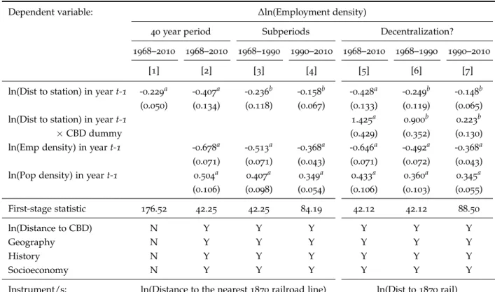
Table1: The effect of rail transit on employment growth and decentralization, TSLS estimates

Dependent variable: ∆ln(Employment density)

40year period Subperiods Decentralization?

1968–2010 1968–2010 1968–1990 1990–2010 1968–2010 1968–1990 1990–2010

[1] [2] [3] [4] [5] [6] [7]

ln(Dist to station) in yeart-1 -0.229a -0.407a -0.236b -0.158b -0.428a -0.249b -0.148b

(0.050) (0.134) (0.118) (0.067) (0.133) (0.119) (0.065)

ln(Dist to station) in yeart-1 1.425a 0.900b 0.223b

×CBD dummy (0.429) (0.352) (0.130)

ln(Emp density) in yeart-1 -0.678a -0.513a -0.368a -0.646a -0.492a -0.368a

(0.071) (0.071) (0.043) (0.071) (0.072) (0.043)

ln(Pop density) in yeart-1 0.504a 0.407a 0.349a 0.433a 0.360a 0.345a

(0.106) (0.098) (0.054) (0.106) (0.103) (0.055) First-stage statistic 176.52 42.25 42.25 84.19 42.12 42.12 88.50 ln(Distance to CBD) N Y Y Y Y Y Y Geography N Y Y Y Y Y Y History N Y Y Y Y Y Y Socioeconomy N Y Y Y Y Y Y

Instrument/s: ln(Distance to the nearest1870railroad line) ln(Dist to1870rail)

ln(Dist1870rail)×CBD dummy

Notes: 1300 observations in each regression. Robust standard errors are in parentheses. a, b, and c indicates

significant at1,5, and10percent level, respectively.

The estimated coefficients are displayed in Table 1. In columns 1 and 2, the results for the

whole1968–2010period show that the further away a municipality was from a station, the more

its employment density decreased over the period. To put it differently, these estimates reveal that proximity to rail stations fosters employment growth. Decomposing the total period into two

7

The Digital Atlas of Roman and Medieval Civilizations (DARMC) is a website with free GIS maps for the Roman and medieval worlds (seedarmc.harvard.edu/icb/icb.do).

(9)

subperiods (columns 3and4) shows that this concentration around transit is observable both at

the beginning and at the end of the period, but is more marked in the early years of the period (1968to1990), corresponding to the first and main improvements of the railway network.

Evidence of the decentralization process described in the previous subsection is presented in columns 5 to 7, in which the regressions control for the interaction between the distance

to the closest railway station and a dummy variable indicating the CBD. The coefficients for this interaction term reveal that conditional on belonging to the CBD (the 20 arrondissements of

Paris), getting closer to rail station tends to reduce employment over time, a clear sign of job decentralization.

Finally, we can note that the estimated coefficients for proximity to rail stations remain stable when we control for the proximity to highway ramps, as reported in AppendixD. These regres-sions also show that the distance to the closest highway ramp does not relate to employment growth.

3. Is Paris decentralization diffuse or clustered around subcenters?

After establishing that the Paris metropolitan area went through a job decentralization process related to the improvement of the railway transportation network, we now want to characterize the spatial pattern of this process: Does decentralization follow a polycentric spatial pattern, reinforcing existing secondary centers (subcenters) and/or fostering the emergence of new ones? Or does it rather reflect a dispersed spatial pattern, in which suburban land is occupied by low-density settlements? To answer these questions, we first identify subcenters for each census year between1968and2010before analyzing the evolution of employment inside these subcenters

versus noncentral locations between1968and2010. 3.1 Identifying and characterizing subcenters

An employment subcenter is a place with a significantly larger employment density than nearby locations that has a significant effect on the overall spatial distribution of jobs. We identify employment subcenters using the method first developed by McDonald and Prather (1994) and

improved by McMillen (2001). The main idea is to estimate densities following a monocentric

spatial pattern. The predicted densities obtained are then substracted from the corresponding real densities. The positive and statistically significant residuals are finally selected.

While McDonald and Prather (1994) estimate by OLS a two dimensional density function

(log of employment density on the distance to CBD), as in Figure 1, McMillen (2001) suggests

estimating a three-dimensional density function (log of employment density on north-south and east-west distances to CBD) with a Locally Weighted Regression (LWR). Both improvements allow to take into account geographical differences, which, in terms of the spatial pattern of densities, can occur in any direction from the CBD (e.g. steeper density gradients on the north side than on the south side of the city). They additionally allow to define any type of monocentric spatial pattern: concave, convex or linear.

(10)

We therefore estimate the following employment density function:

ln(Employment density)=γ0+γ1×north-south distance to CBD +γ2×east-west distance to CBD

(2)

where density is measured as jobs per hectare, and distances are in kilometers. The CBD is defined as the 20 arrondissementsthat make up the city of Paris. Distance to CBD is the distance

to the centroid of the4th arrondissement(corresponding to the town-hall of Paris).

Since our estimates are based on LWR, we need to define a bandwidth. AsMcMillen (2001)

points out, this is a critical choice because we need a monocentric benchmark. We experiment with alternative window sizes ranging from 1% to 9% and from 10% to 90% (see Table C.1 in

AppendixC). After visual inspection, we find that the first monocentric spatial structure appears when the nearest50% observations are included in each local regression. Interestingly, this is the

value used by McMillen (2001) for some US cities. We also experimented with a selection rule

based on the Akaike information criterion. However, the selected window size (7%) was clearly

related to a polycentric spatial structure (see and compare Tables C.1andC.2in AppendixC).

Second, for each site we compute the residual as the difference between the log of real employment density and the estimated log of employment density. We then select those that are significantly positive, according to their own standard errors that can vary over space (McMillen,

2001). We use two critical thresholds, 1.96 and 1.64, that are associated with a 5% and a 10%

significance level, respectively.

Finally, we group the selected sites in subcenters when they are contiguous. We use a "queen" criterion for contiguity: two sites (municipalities) are contiguous if they share at least one point in their boundaries. SeeMcMillen(2001,2003) andGarcia-López(2010) for further details on this

procedure.

This methodology enables us to identify subcenters for each census year between 1968 and 2010, which are described in Table 2. For each year, we report two figures, corresponding to

subcenters identified using positive residuals significant at the5and at the10% level, respectively.

From Panel A, we can see that the number of subcenters identified at the5% level (respectively, at

the10% level) increased from20to26(respectively from21to35) between1968and2010. Panel B

reveals that these subcenters hosted1,756,000jobs in2010(respectively1,979,000), corresponding

to an increase of about 600,000 jobs since 1968(respectively 560,000). We can also observe that

subcenters are heterogeneous in terms of size, with an increasing number of large subcenters (more than20,000jobs), in line with the decentralization process: in1968, between15% and20%

of subcenters hosted more than 20,000 jobs, contrasting with a range of 42% to 50% in 2010.

Finally, we want to emphasize that the number of subcenters and the number of jobs in the subcenters do not differ much whether the subcenters are identified using positive residuals a the

5% level or at the 10% level. We will henceforth use the subcenters identified at the 10% level in

(11)

Table2: Employment subcenters in metropolitan Paris,1968–2010

1968 1975 1982 1990 1999 2010

Resid. significant at: 5% 10% 5% 10% 5% 10% 5% 10% 5% 10% 5% 10%

Panel A: Number of subcenters

All subcenters 20 21 26 27 30 32 29 34 31 34 26 35

≥10,000jobs 7 8 13 14 18 16 19 21 19 19 19 23

≥20,000jobs 3 4 8 7 9 12 13 13 13 12 13 15

Panel B: Jobs (’000) in subcenters

All subcenters 1,152 1,419 1,319 1,667 1,237 1,665 1,373 1,788 1,441 1,782 1,756 1,979

≥10,000jobs 1,088 1,350 1,254 1,601 1,169 1,582 1,326 1,720 1,369 1,693 1,714 1,909

≥20,000jobs 1,022 1,290 1,184 1,501 1,040 1,513 1,252 1,618 1,281 1,602 1,624 1,788

Note:LWR estimates use a window size of0.5(i.e., the nearest of the50% observations).

Table3 further describes the identified subcenters (at the10% level) regarding the number of

municipalities they encompass. We can first notice that the number of municipalities that form a subcenter of their own or that are part of a subcenter is quite stable, from 88 in 1968 to 89 in 2010, oscillating between 93 to 97 in the meantime. The last line of Panel A illustrates a certain

stability in the composition of subcenters: among all the municipalities belonging to a subcenter,

57 are constantly identified as a subcenter (or as part of a subcenter) over time. The remaining

municipalities may have emerged as part of a subcenter at some point, or, alternatively, stopped being considered as such.

Table3: Municipalities in employment subcenters in metropolitan Paris, 1968–2010

1968 1975 1982 1990 1999 2010

Panel A: All subcenters

All municipalities 88 97 93 95 95 89

Emerging as (part of) subcenters – 18 7 11 12 5

Disappearing as (part of) subcenters – 9 11 9 12 11

Always in subcenters 57 57 57 57 57 57

Panel B: Subcenters≥10,000jobs

Panel C: Subcenters≥20,000jobs

Note:Employment subcenters identified usingMcMillen(2001)’s method with a LWR window size of50%, and for

(12)

3.2 The spatial pattern of decentralization

In order to determine the spatial pattern of employment decentralization, we now compare the evolution of employment inside and outside these subcenters over the period of interest.

Table4displays the number of jobs in each type of area (e.g. subcenter versus non-central) for

all census years (columns1to6), and the corresponding variation between1968and2010(column 7). In the non-constant geographypanel (Panel A), the figures correspond to all subcenters and all

non-central locations identified at a given date, some of them having appeared or disappeared as subcenters since the previous wave. In other words, the geography is not constant in the sense that the municipalities included in the Subcenters category (or, by symmetry, in the Non-central

category) differ between two points in time. By contrast, the figures reported in the constant geography panel (Panel B) correspond to geographical zones that are fixed over time according to various criteria. Here, the geography is constant in the sense that the municipalities included in each type of zone considered are the same at each point in time. For instance, the Always subcenters category includes the 57 municipalities that are identified as a subcenters (or part of

one) in all six years, while the Always noncentral group refers to municipalities that were not identified as (part of) a subcenter in anyyear. Similarly, the 35municipalities identified as (part

of) a subcenter in 2010 are included in the Subcenters in 2010 group for all years, even if they

may not have been (part of) a subcenter before2010, while the remaining1,265municipalities go

under theNon-central in2010label. Finally,1968Non-central to subcentersrefers to municipalities that were non-central in1968 and, at some point, became (part of) a subcenter and remained as

such until 2010, while municipalities that were (part of) a subcenter in1968 and, at some point,

lost this status up to2010are labeled as1968Subcenters to non-central.

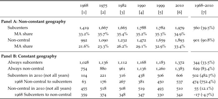
Table4: The spatial pattern of decentralized employment in metropolitan Paris,1968–2010

1968 1975 1982 1990 1999 2010 1968–2010

[1] [2] [3] [4] [5] [6] [7]

Panel A: Non-constant geography

Subcenters 1,419 1,667 1,665 1,788 1,782 1,979 560(39.5%)

MA share 33.2% 35.7% 35.4% 35.2% 35.3% 34.9%

Non-central 992 1,090 1,232 1,472 1,659 1,893 901(90.8%)

MA share 21.6% 23.3% 26.2% 29.1% 32.9% 33.4%

Panel B: Constant geography

Always subcenters 1,028 1,136 1,112 1,168 1,183 1,372 344(33.5%)

Always non-central 754 880 961 1,136 1,260 1,383 629(83.4%)

Subcenters in2010(not all years) 104 221 316 438 506 606 502(482.7%) 1968Non-central to subcenters 63 176 267 381 450 537 474(752.4%)

Non-central in2010(not all years) 455 518 508 519 493 510 55(12.1%) 1968Subcenters to non-central 359 374 348 347 330 342 -17(-4.7%)

Note: Employment values are thousands of jobs. Growth rates are in parentheses. Employment subcenters identified usingMcMillen(2001)’s method with a LWR window size of50%, and for positive residuals significant

(13)

The figures reported in Table4reveal several interesting characteristics of the decentralization

process. We can see from the non-constant geography panel (Panel A) that subcenters always concentrate around a third of all jobs in the Paris metropolitan area. Non-central municipalities represented around one fifth of all jobs in the metropolitan area in 1968, but up to one third

in 2010(while they include roughly1,200municipalities out of the 1,300under study). Since the

municipalities included in a given category vary from one year to another, it is however difficult to compare the employment shares at different dates and to appreciate the increase in employment share for non-central municipalities in this panel.

For this reason, we now turn to the figures of the constant geography panel (Panel B). We can first note that the number of jobs located in the 57 municipalities that are always identified as

(part of) a subcenter has increased over time, from 1,028thousands in 1968 to 1,372 thousands

in 2010, which corresponds to a growth rate of33.5% (column7). The increase in the number of

jobs inalways non-centralmunicipalities is even more striking: this subset of municipalities saw its number of jobs grow by83.4% over the period, with629thousands additional jobs. Although this

increase in the number of jobs is almost twice as large as the one experienced byalways subcenters

municipalities, we must bear in mind that the latter represent less than 5% of municipalities.

We can also observe that the magnitude of employment growth in 2010 subcenters and in 1968

noncentral to subcentersis very large, both in absolute and relative terms.

4. Does rail transit cause subcenter formation?

After analyzing the job decentralization process in the Paris metropolitan area, we now turn to the most important part of this paper, where we contribute to the literature by establishing that rail transit causes subcenter formation. To answer to this key question, we proceed in two steps. We first investigate whether the existence of a rail station in a suburban municipality increases the probability that this municipality becomes (part of) a subcenter. Then, we examine whether proximity to rail stations also increases the likelihood of becoming (part of) a subcenter, even when the station is not built on the municipal ground.

In both steps, our empirical strategy consists in regressing the probability that a municipality becomes a subcenter on a rail station variable. In section 4.1, where we explore the role of the

existence of a rail station, this variable indicates whether there is a station within the adminis-trative boundaries of the municipality or the number of stations and lines in the municipality. Alternatively, in section 4.2, this variable measures the distance between a municipality and the

closest station. All regressions include controls for the characteristics related to Paris urban spatial structure (geography, history, and socio-economic variables) that were used in Equation (1). The

(14)

Prob(subcenter)_t =β0+δ1×Rail station variablet +δ2×ln(densities)t+δ3×ln(distance to CBD) +

∑

i (δ_4,_i×geography_i) +

∑

i (δ_5,_i×history_i) +

∑

i (δ_6,_i×socioeconomy_i_,_t) (3)

In order to correct for the potential biases related to the endogenous location of rail stations, we use the distance to the nearest1870railroad line (Section4.1) and a dummy variable indicating

whether a given municipality was crossed by a rail (a train line) in 1870(Section 4.2) as

instru-ments, as explained in Section 2 and documented and discussed in Appendix B. However, the

use of these historical instruments comes with a caveat: since they are time invariant, we can not estimate using panel data techniques. As a result, we pool all observations together, irrespective of the year, and include year fixed effects in our regressions. As a robutness, we also run some cross-sectional regressions.

4.1 Do rail stations lead to subcenters?

In order to establish whether the existence of a rail station in a suburban municipality increases the probability that this municipality becomes (part of) a subcenter, we estimate Eq. (3) using the

subsample of the 1,280suburban municipalities (excluding the20arrondissementsof Paris).

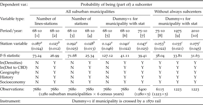
The marginal effects of the corresponding (second-stage) results are displayed in Table 5.

Columns1to7presents results estimated on the full subsample of all suburban municipalities. In

columns1 and2, the station variable represents the number of lines times station, which counts

the total number of lines having a stop in a municipality (it can be seen as a weighted count of the number of stations). The station variable then simply counts the number of stations in columns3

and4, and indicates the existence of a station in columns 5to7.8 We will restrict our comments

on the specifications that control for the geographical and historical characteristics, after noting that the marginal effects are significantly reduced in the conditional regressions.

Column 4 indicates that an additional station increases the probability that the municipality

becomes (part of) a subcenter by 2.8%. This effect is exactly the same as that of having an

additional line stopping in the municipality (column2). This does not come as a surprise given

that most of the suburban municipalities are only crossed by one train line, so that the number of lines-stations is actually very close to the number of stations.

Regarding the existence of a station, we estimate a slightly larger effect, around 4% over the

whole period (column 6). This difference in magnitude can be interpreted as saying that what matters the most in explaining subcenter formation is the mere existence of a train station, not the number of stations. This effect increases to 4.7% when we focus on the 1975-2010 period (column 7),

8

Therefore, if a municipality has two stations, withn1lines stopping in one station andn2 lines in the other one,

the "number of lines-stations" variable takes a value ofn1+n2, the "number of stations" variable takes a value of2,

(15)

suggesting either that the effect is delayed in time, or that the transportation system built after

1975(mostly the RER) explains a larger part of the overall effect.

Table5: The effect of rail stations on subcenter formation, IV Probit - Marginal effects

Dependent var.: Probability of being (part of) a subcenter

All suburban municipalities Without always subcenters Variable type: Number of Number of Dummy=1for Dummy=1for

lines-stations stations municipality with stat municipality with stat Period/year: 68-10 68-10 68-10 68-10 68-10 68-10 75-10 75-10 1975 2010 [1] [2] [3] [4] [5] [6] [7] [8] [9] [10] Station variable 0.087a 0.027b 0.092a 0.028b 0.142a 0.040c 0.047c 0.053b 0.035c 0.075c (0.024) (0.012) (0.025) (0.013) (0.046) (0.022) (0.025) (0.022) (0.021) (0.045) F-S statistic 73.24 26.99 71.68 25.34 127.12 41.11 39.41 38.04 33.81 31.63 ln(Densities) N Y N Y N Y Y Y Y Y ln(Dist to CBD) N Y N Y N Y Y Y Y Y Geography N Y N Y N Y Y Y Y Y History N Y N Y N Y Y Y Y Y Socioeconomy N Y N Y N Y Y Y Y Y Observations: 7680 7680 7680 7680 7680 7680 6400 6115 1223 1223

(1280suburban municipalities×6census years) (1280×5) (1223×5)

Instrument: Dummy=1if municipality is crossed by a1870rail

Notes: Regressions in columns1to8include year effects. Robust standard errors and are in parentheses (and are

clustered by municipality in regressions in columns1to8). a,b, andc indicates significant at1,5, and10percent

level, respectively.

In order to dig further into this time variation, we focus on the1975-2010period in columns 8 to 10, taking the municipalities systematically identified as subcenters out of the sample. The

estimated effect over the period jumps to 5.3% (column 8) confirming the idea of an reinforced

effect in the most recent period (the effect goes from3.5% in1975to7.5% in2010(columns9and 10), but the difference is not significant).

We check the robustness of our results in Appendix E. In Table E.1 Panel A we show that

estimates are robust to subcenter size and definition: the effect is always between 3.5% and 4.4%, whether we focus on municipalities of more or less than 50,000 inhabitants (columns 1

and 2), and whether we rely on subcenters identified using the 5% criterion (columns 3 and4)

(instead of10% in the main results). In TableE.2Panel A we test the validity of our identification

strategy by dropping some observations of municipalities. Since the1870 railroad network was

probably planned to serve the most important municipalities during the 19th centuries, we first

drop municipalities that were important. We do not have population data at the municipality level for these years, as a result we use our historical dummy variables that signal the most important towns through history. That is, we drop municipalities that were Roman settlements and/or major towns during the10th and19th centuries and/or with a monastery built between the12th

and16th centuries (columns 1and2). Alternatively, we also drop observations of municipalities

with a rail station built during the 19th century (columns 3 adn 4). In both cases, results still

show a significant and positive effect of having a rail station on the probability of becoming (part of) a subcenter.

(16)

We now refine our results by investigating the train station effect, looking alternatively at two different train types: suburban trains versus RER. The corresponding results are displayed in columns 1 to 4 of Table 6 for the former train type, and in columns 5 to 8 for the latter. Over

the1968-2010period, we estimate that the presence of a suburban train station in a municipality

increases the likelihood that it becomes a subcenter by 3.4% (column 2). As before, this effect

slightly increases (to 3.9%) when we focus on the1975-2010period (column 3), and goes up to 4.4% once we exclude municipalities that are always identified as a subcenter (column4). These

figures are of the same order of magnitude, although slightly lower than the estimates obtained for all train types in the previous table (the corresponding figures being 4%, 4.7% and 5.3%

respectively).

Table6: The effect of train and RER stations on subcenter formation, IV Probit - Marginal effects

Train stations RER stations

Without Without

All suburban municipalities always sub All suburban municipalities always sub Period: 68-10 68-10 75-10 75-10 68-10 68-10 75-10 75-10 [1] [2] [3] [4] [5] [6] [7] [8] Station dummy 0.175a 0.034c 0.039c 0.044a 0.680a 0.140a 0.135a 0.102a (0.049) (0.020) (0.021) (0.017) (0.191) (0.046) (0.036) (0.034) F-S statistic 114.12 44.56 43.62 36.83 29.43 10.74 9.91 11.21 ln(Densities) N Y Y Y N Y Y Y ln(Dist to CBD) N Y Y Y N Y Y Y Geography N Y Y Y N Y Y Y History N Y Y Y N Y Y Y Socioeconomy N Y Y Y N Y Y Y Observations: 7680 7680 6400 6115 7680 7680 6400 6115 (1280×6years) (1280×5) (1223×5) (1280×6years) (1280×5) (1223×5)

Instrument: Dummy=1if municipality is crossed by a1870rail

Notes: All regressions include year effects. Robust standard errors are clustered by municipality and are in parentheses. a,b, andcindicates significant at1,5, and10percent level, respectively.

On the other hand, the RER results reveal that this particular type of train has a much stronger impact on subcenter formation. The existence of a RER station is indeed found to increase the probability of becoming (part of) a subcenter by 14% over the 1968-2010 period (column 6), an

effect about four times as large as for suburban trains. Interestingly, looking at the later period (after1975) does not show a significantly different effect (13.5%, column7).

4.2 Does proximity to rail stations lead to subcenters?

We now want to examine the effect of the distance to a train station on subcenter formation. This presents a double advantage: it enables us to measure the spatial effect of the presence of

(17)

a train station, and allows to consider the effect of a train station on municipalities that do not possess any. In other words, we investigate whether the effect of a rail station can go beyond the boundaries of the municipality where the station is located.

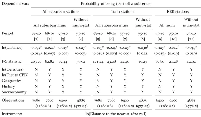
To this aim, we now use the distance (in log) of a municipality’s centroid to the closest train station as thetrain station variable. The main conclusion to be drawn from the results reported in Table 7 is that train stations have extended spatial effects: being closer to a station increases the

probability to be (part of) a subcenter, even for municipalities without any station.

Table7: The effect of rail proximity on subcenter formation, IV Probit - Marginal effects

All suburban stations Train stations RER stations

Without Without Without

All suburban muni muni-stat All suburban muni muni-stat All muni muni-stat Period: 68-10 68-10 75-10 75-10 68-10 68-10 75-10 75-10 75-10 75-10 75-10 [1] [2] [3] [4] [5] [6] [7] [8] [9] [10] [11] ln(Distance) -0.092a -0.024a -0.027a -0.027a -0.105a -0.024a -0.027a -0.030b -0.127a -0.042b -0.049a (0.014) (0.007) (0.007) (0.007) (0.016) (0.009) (0.009) (0.012) (0.017) (0.019) (0.019) F-S statistic 203.20 82.82 82.44 39.92 171.24 43.08 42.40 19.25 87.80 21.28 12.92 ln(Densities) N Y Y Y N Y Y Y N Y Y ln(Dist to CBD) N Y Y Y N Y Y Y N Y Y Geography N Y Y Y N Y Y Y N Y Y History N Y Y Y N Y Y Y N Y Y Socioeconomy N Y Y Y N Y Y Y N Y Y Observations: 7680 7680 6400 4885 7680 7680 6400 4885 6400 6400 4885 (1280×6) (1280×5) (977×5) (1280×6) (1280×5) (977×5) (1280×5) (977×5)

Instrument: ln(Distance to the nearest1870rail)

As in the previous section, we find a very similar effect of the proximity to any type of train or to suburban train alone. In this case, getting closer to a station by one kilometer increases the probability of becoming a subcenter by 2.4% (columns2 and 6), or by 2.7% considering the 1975-2010 period (columns3 and7). On the other hand, the effect of being one kilometer closer

to an RER station is estimated at4.2% (column 10). Therefore, proximity to a station matters in

the suburbanization process, especially for RER station.

We obtain similar results when we restrict our sample to the977suburban municipalities that

do not have any station within their boundaries (columns 4, 8 and 11). This effect, of 3% for

suburban trains and4.9% for RER, confirms the spatially lagged effect of train stations.

Finally, we check that our results are robust to subcenter size (more or less than 50,000

inhabitants) and definition (subcenters identified using the 5% threshold instead of 10%), and

(18)

crossed by railroads during the 19th century. These tests are reported in Tables E.1Panel B and

E.2Panel B in AppendixE.

To summarize the results of this section, two main points can be highlighted. First, train stations do play a role in the subcenter formation process, and this effect is spatially lagged: the existence of a train station increases the probability of becoming part of a subcenter by 4to 5%,

and decreases at a rate of about3% per kilometer. Second, the RER is the type of train having the

most important effect, with a direct effect of around14% for municipalities with a station, and a

spatial decay of about5% per kilometer.

5. Conclusions

In this paper we investigate the effect of railroad construction on the emergence of employment subcenters in metropolitan Paris between 1968 and 2010. Because of the potential endogeneity

problem of railroad provision, we rely on IV estimations that use historical instruments built on the19th century railroad network: a dummy for municipalities crossed by1870railroads, and the

(log) distance to the nearest1870railroad.

We provide descriptive evidence of an employment decentralization process: while the number of jobs grew by 30% in the whole metropolitan area, it declined by7.1% in central and increased

by 65% in suburban municipalities between 1968 and 2010. Simultaneously, we highlight the

important railroad improvements in the same period: the construction of the Réseau Exoress Réginal increased the railroad network with 5 new lines with 587 km and 243 stations. Our

first results confirm that only railroads foster local employment growth: our average estimates reveal that job growth increases with proximity to rail stations. When we focus on central Paris, results confirm that railroads do cause job decentralization: getting closer to a rail station tends to reduce employment over time.

We then focus on the suburbs to study the spatial pattern of job decentralization. We identify employment subcenters and, despite some municipalities emerge as (part of) subcenters whereas others were dropped, the number of subcenters grew from 21 in 1968 to 35 in 2010. Since

employment growth in these subcenters was very intense over the period, we conclude that employment decentralization in Paris is more clustered around subcenters than diffuse, thus reinforcing the polycentric nature of the city.

Finally, we investigate whether railroads cause the emergence of employment subcenters in Paris and our results confirm the causal effect. On average, the probability of a suburban municipality of being (part of a) subcenter increases by 5% if the municipality has a rail station

within its boundaries, or by3% if, although not having a rail station, municipality proximity to a

rail station increases by 10%. Results for the RER confirm its effect is stronger: a10% and a 5%

increase in the probability of becoming (part of a) subcenter if the municipality has a RER station or if municipality proximity to a RER station increases by10%, respectively.

The contribution of the paper is relevant because, as far as we know, it provides the first empirical evidence on the causal effect of transportation (railroad) on subcenter formation. Fur-thermore, these new results are useful for urban planners facing and dealing the consequences

(19)

of urban growth and, in particular, of population suburbanization, employment decentralization and urban sprawl: while these phenomena might reduce city’s agglomeration economies (Glaeser and Kahn,2004), the emergence of employment subcenters can potentially compensate and even

overcome these loses by offering new agglomeration economies and avoiding CBD’s congestion costs (McMillen,2004).

References

Anas, Alex and Ikki Kim.1996. General Equilibrium Models of Polycentric Urban Land Use with

Endogenous Congestion and Job Agglomeration. Journal of Urban Economics40(2):232–256.

Arribas-Bel, Daniel and Fernando Sanz-Gracia.2014. The validity of the monocentric city model

in a polycentric age: US metropolitan areas in 1990, 2000 and 2010. Urban Geography 35(7): 980–997.

Bairoch, Paul. 1988. Cities and Economic Development: From the Dawn of History to the Present.

University of Chicago Press.

Baum-Snow, Nathaniel. 2007. Did highways cause suburbanization? The Quarterly Journal of Economics122(2): 775–805.

Baum-Snow, Nathaniel. 2010. Changes in transportation infrastructure and commuting patterns

in us metropolitan areas1960-2000.American Economic Review Papers & Proceedings100: 378–382.

Baum-Snow, Nathaniel.2014. Urban transport expansions, employment decentralization, and the

spatial scope of agglomeration economies. Mimeo.

Baum-Snow, Nathaniel, Loren Brandt, J. Vernon Henderson, Matthew A. Turner, and Qinghua Zhang.2015. Roads, railroads and decentralization of chinese cities. Mimeo.

Berliant, Marcus, Shin-Kun Peng, and Ping Wang. 2002. Production Externalities and Urban

Configuration. Journal of Economic Theory104(2):275–303.

Berliant, Marcus and Ping Wang. 2008. Urban growth and subcenter formation: A trolley ride

from the Staples Center to Disneyland and the Rose Bowl. Journal of Urban Economics 63(2): 679–693.

Boarnet, Marlon G. 1994. The monocentric model and employment location. Journal of Urban Economics36(1):79–97.

Bollinger, Christopher and Keith Ihlanfeldt. 1997. The impact of rapid rail transit on economic

development: The case of atlanta’s marta. Journal of Urban Economics42(2):179–204.

Bollinger, Christopher and Keith Ihlanfeldt.2003. The intraurban spatial distribution of

employ-ment: which government interventions make a difference? Journal of Urban Economics 53(3): 396–412.

Duranton, Gilles and Diego Puga.2015. Urban land use. In Gilles Duranton, J. Vernon Henderson,

and William C. Strange (eds.)Handbook of Regional and Urban Economics Volume5. Amsterdam: North-Holland,467–560.

Duranton, Gilles and Matthew A. Turner.2012. Urban growth and transportation. The Review of Economic Studies79(4): 1407–1440.

(20)

Fujita, Masahisa and Hideaki Ogawa.1982. Multiple equilibria and structural transition of

non-monocentric urban configurations. Regional Science and Urban Economics12(2): 161–196.

Garcia-López, Miquel-Àngel. 2010. Population suburbanization in Barcelona, 1991-2005: Is its

spatial structure changing? Journal of Housing Economics 19(2):119–132.

Garcia-López, Miquel-Angel. 2012. Urban spatial structure, suburbanization and transportation

in Barcelona. Journal of Urban Economics72(2–3):176–190.

Garcia-López, Miquel-Àngel, Camille Hémet, and Elisabet Viladecans-Marsal.2015a. How does

transportation shape intrametropolitan growth? an answer from the regional express rail. Working paper2015/20, IEB.

Garcia-López, Miquel-Àngel, Adelheid Holl, and Elisabet Viladecans-Marsal. 2015b.

Suburban-ization and highways in Spain when the Romans and the Bourbons still shape its cities. Journal of Urban Economics85(0):52 –67.

Garcia-López, Miquel-Àngel and Ivan Muñiz. 2013. Urban spatial structure, agglomeration

economies, and economic growth in barcelona: An intra-metropolitan perspective. Papers in Regional Science92(3):515–534.

Garcia-López, Miquel-Àngel, Albert Solé-Ollé, and Elisabet Viladecans-Marsal.2015. Does zoning

follow highways? Regional Science and Urban Economics53(C):148–155.

Genevieve, Giuliano, Christian L. Redfearn, Ajay Agarwal, and Syvia He.2012. Network

accessi-bility and employment centers. Urban Studies49(1): 77–95.

Giuliano, Genevieve and Kenneth A. Small.1991. Subcenters in the Los Angeles region. Regional Science and Urban Economics21(2):163–182.

Giuliano, Genevieve and Kenneth A. Small. 1999. The determinants of growth of subcenters. Journal of Transport Geography7: 189–201.

Glaeser, Edward L. and Matthew E. Kahn.2001. Decentralized employment and the

transforma-tion of the American city. In W.G. Gale and J.R. Pack (eds.)Brookings-Wharton Papers on Urban Affairs:2001. Brookings Institution Press,1–47.

Glaeser, Edward L. and Matthew E. Kahn. 2004. Sprawl and urban growth. In J. Vernon

Henderson and Jacques-François Thisse (eds.)Handbook of Regional and Urban Economics Volume

4. Amsterdam: North-Holland,2481–2527.

Helsley, Robert W. and Arthur M. Sullivan.1991. Urban subcenter formation. Regional Science and Urban Economics21(2):255–275.

Henderson, Vernon and Arindam Mitra. 1996. The new urban landscape: Developers and edge

cities. Regional Science and Urban Economics26(6): 613–643.

Henderson, Vernon and Eric Slade. 1996. Development games in non-monocentric cities. Journal of Urban Economics34(2):207–229.

Lucas, Robert E. and Esteban Rossi-Hansberg.2002. On the internal structure of cities. Economet-rica70(4): 1445–1476.

Martí-Henneberg, Jordi. 2013. European integration and national models for railway networks

(21)

Mayer, Thierry and Corentin Trévien.2015. The impacts of urban public transportation. Evidence

from the Paris metropolitan area. Working Paper g2015/03, INSEE.

McDonald, John F. and Paul J. Prather.1994. Suburban employment centers: The case of Chicago. Urban Studies31(2): 201–218.

McMillen, Daniel P. 2001. Nonparametric employment subcenter identification. Journal of Urban Economics50(3):448–473.

McMillen, Daniel P.2003. Identifying sub-centres using contiguity matrices. Urban Studies 40(1): 57–69.

McMillen, Daniel P. 2004. Employment densities, spatial autocorrelation, and subcenters in large

metropolitan areas. Journal of Regional Science44(2): 225–244.

McMillen, Daniel P. and Stefani C. Smith. 2003. The number of subcenters in large urban areas. Journal of Urban Economics53(3):321–338.

Michaels, Guy. 2008. The effect of trade on the demand for skill: Evidence from the interstate

(22)

Appendix A. 1968-2010: Decentralization and transportation improvements

Table A.1: Employment trends in metropolitan Paris,1968–2010

1968 1975 1982 1990 1999 2010 1968–2010 Metropolitan area 4,277 4,675 4,705 5,076 5,042 5,669 1,392(32.6%) CBD (municipality of Paris) 1,936 1,918 1,808 1,815 1,601 1,798 -138(-7.1%) MA share 45.3% 41.0% 38.4% 35.8% 31.8% 31.7% Suburban municipalities 2,341 2,757 2,897 3,261 3,441 3,871 1,530(65.4%) MA share 54.7% 59.0% 61.6% 64.2% 68.2% 68.3%

Note:Employment values are thousands of jobs. Growth rates are in parentheses.

(23)

Appendix B. Rail transit in Paris: Past and present

One of the main purposes of this paper is to evaluate whether and to what extent transportation has fostered the emergence of employment subcenters in metropoliran Paris. However, first we need to deal with an identification issue because transportation and its improvements are not placed randomly. On the contrary, they are endogenous to employment and/or population location and growth. Planners may for instance decide to improve the connection of deprived areas in order to boost their economic activity or attract population. In order to address this issue, we adopt an instrumental variable approach in which some variables, named instruments, are used as sources of exogenous variation for our transportation endogenous variables.

Recent literature highlights the advantages in terms of exogeneity and relevance of using ’historical’ and ’planned’ instruments. For instance, Baum-Snow (2007), Michaels (2008) and

Duranton and Turner(2012) use the1947plan of the interstate highway system as an instrument

for modern highways in the US, and Duranton and Turner(2012) additionally rely on the1898

railroad network. Garcia-López (2012) uses the ancient Roman roads, and the19th century main

road and railroad networks as instruments for highways and railroads in metropolitan Barcelona. Finally,Garcia-Lópezet al.(2015b) use the ancient Roman roads and the1760Bourbon roads (post

routes) to instrument current highways in Spain.

Following the above mentioned literature, we instrument modern railroads in metropolitan Paris with a historical instrument, the1870railroad network. The first French railroads were built

at the beginning of the19th century, but slightly later than in the UK due to Napoleon wars: the

first line connecting Paris to a city located 18 km away (Saint-Germain) was not opened before 1837. In1870, the railroad network was based on698km of railroad lines. Due to the high levels

of centralization in France, it had a star-shaped form centered around Paris (FigureB.1).

Figure B.1: The1870railroads

(24)

Is the1870rail network a valid instrument?

As above mentioned, the fact that modern roads and railroads were built following ancient infrastructures has already been argued and used in the literature. Common sense would suggest that in France as well, past infrastructures shape current ones due to practical reasons: it is easier and cheaper to build new transportation infrastructures as an improvement of old ones for instance, or close to them (Duranton and Turner,2012). We now test empirically the credibility of

this assumption in the context of the metropolitan area of Paris. To do so, we conditially regress our endogenous rail variables on their historical counterparts and some control variables:

2010Rail transit variable=_α0+_α

1×1870rail transit variable +

∑

i

(α_2,_i×control variables) (B.1)

It is important to point out the importance of the control variables, in particular geography and history. Although ancient transportation infrastructures may be exogenous because of the length of time since they were built, the significant changes undergone by society and economy in the intervening years, and, in particular, because neither of them were built to anticipate employment and population changes in a distant future; it is also true that other factors such as the geography are likely to have influenced the construction and location of both ancient and modern transportation infrastructures for obvious reasons related to the feasibility and convenience of infrastructure building. From this point of view, it is crucial to include geographic characteristics such as altitude, index of terrain ruggedness, and elevation range as controls to comply with the exogeneity condition.

On the other hand, it is equally important to control for the historical context, since it may explain both the presence of former infrastructure and the economic importance of present-days municipalities. In order to fulfill the exclusion restriction, and because there are no historical employment and population data at the municipal level prior to 1962and 1968, we control for

history by including the population level in 1962 and dummy variables indicating (1) whether

municipalities were Roman settlements, (2) whether they used to be major towns between the 10th and the15th centuries and (3) between the16th and the19th centuries, and (4) whether they

had a monastery built between the12th and16th centuries. These dummy variables come from

theDigital Atlas of Roman and Medieval Civilizations, with the exception of the major cities of the16th to19th centuries which are identified inBairoch(1988). To put it differently, we assume conditionalexogeneity of the proposed instruments, as suggested by (Duranton and Turner,2012).

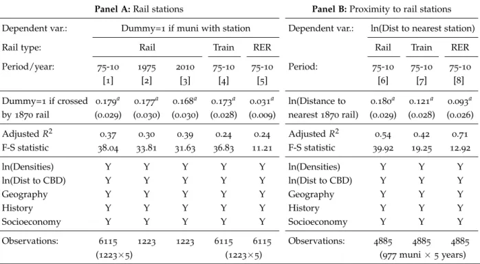
Regarding the relevance of our potential instruments, TableB.1 shows results for versions of

Eq. (B.1) in which we analyze the relationship between modern and past railroads in terms of the

presence of stations and proximity to them. In particular, in Panel A, we study whether suburban municipalities crossed by a 1870rail receive a rail stations. In all cases (pooled vs. cross section

regressions in columns 1 and 2-3, all railroads vs. train and RER regressions in columns1 and 4-5) we find significant and positive coefficients for the presence of 1870 rails. In Panel B, we

(25)

nearest modern rail. Conditional on control variables, estimated coefficients for the1870distance

variable are positive and highly significant. As a whole, results in Table B.1 clearly show that

historical rails matter for modern rail construction and location.

Table B.1: Modern rail transit as a function of past rail transit, OLS estimates Panel A:Rail stations Panel B:Proximity to rail stations Dependent var.: Dummy=1if muni with station Dependent var.: ln(Dist to nearest station)

Rail type: Rail Train RER Rail Train RER

Period/year: 75-10 1975 2010 75-10 75-10 Period: 75-10 75-10 75-10

[1] [2] [3] [4] [5] [6] [7] [8]

Dummy=1if crossed 0.179a 0.177a 0.168a 0.173a 0.031a ln(Distance to 0.180a 0.121a 0.093a

by1870rail (0.029) (0.030) (0.030) (0.028) (0.009) nearest1870rail) (0.029) (0.028) (0.026)

AdjustedR2 ₀_.₃₇ ₀_.₃₀ ₀_.₃₉ ₀_.₂₄ ₀_.₂₄ _Adjusted_R2 ₀_.₅₄ ₀_.₄₂ ₀_.₇₁ F-S statistic 38.04 33.81 31.63 36.83 11.21 F-S statistic 39.92 19.25 12.92 ln(Densities) Y Y Y Y Y ln(Densities) Y Y Y ln(Dist to CBD) Y Y Y Y Y ln(Dist to CBD) Y Y Y Geography Y Y Y Y Y Geography Y Y Y History Y Y Y Y Y History Y Y Y Socioeconomy Y Y Y Y Y Socioeconomy Y Y Y Observations: 6115 1223 1223 6115 6115 Observations: 4885 4885 4885 (1223×5) (1223×5) (977muni×5years)

Notes: Pooled regressions in Columns1and4to8include year effects. Cross section regressions in Columns2and 3include a constant. Columns1to3, Columns4and5, and Columns6to8show first-stage results for regressions

in Table 5Columns 8to10, Table6Columns 4 and8, and Table7Columns 4, 8 and11, respectively. Robust

standard errors are clustered by municipality and are in parentheses. a,b, andcindicates significant at1,5, and10

(26)

Appendix C. LWR and urban spatial structure in metropolitan Paris,1968–2010

Table C.1: Employment spatial structure and LWR: A benchmark to identify subcenters

1968 1975 1982 1990 1999 2010

1% LWR Benchmark Polycentric Polycentric Polycentric Polycentric Polycentric Polycentric 3% LWR Benchmark Polycentric Polycentric Polycentric Polycentric Polycentric Polycentric 5% LWR Benchmark Polycentric Polycentric Polycentric Polycentric Polycentric Polycentric 7% LWR Benchmark Polycentric Polycentric Polycentric Polycentric Polycentric Polycentric 9% LWR Benchmark Polycentric Polycentric Polycentric Polycentric Polycentric Polycentric 10% LWR Benchmark Polycentric Polycentric Polycentric Polycentric Polycentric Polycentric 30% LWR Benchmark Polycentric Polycentric Polycentric Polycentric Polycentric Polycentric 50% LWR Benchmark Monocentric Monocentric Monocentric Monocentric Monocentric Monocentric 70% LWR Benchmark Monocentric Monocentric Monocentric Monocentric Monocentric Monocentric 90% LWR Benchmark Monocentric Monocentric Monocentric Monocentric Monocentric Monocentric

Table C.2: Employment spatial structure and LWR: Akaike information criterion

1968 1975 1982 1990 1999 2010

1% LWR Akaike inf. crit. 746 767 770 778 774 782

70% LWR Akaike inf. crit. 1081 1112 1094 1109 1067 1120 90% LWR Akaike inf. crit. 1284 1331 1318 1346 1301 1364

(27)

Appendix D. Do rails and highways jointly foster local growth in Paris?

Table D.1: The effect of rail transit and highways on employment growth, TSLS estimates

Dependent variable: ∆ln(Employment density)

Period: 1968–2010 1968–1990 1990–2010

[1] [2] [3]

ln(Dist to rail station) in yeart-1 -0.446a -0.276b -0.165c

(0.123) (0.110) (0.089)

ln(Dist to highway ramp) in yeart-1 -0.090 -0.092 -0.314

(0.126) (0.105) (0.202)

ln(Emp density) in yeart-1 -0.677a -0.512a -0.381a

(0.071) (0.071) (0.041)

ln(Pop density) in yeart-1 0.478a 0.380a 0.308a

(0.101) (0.094) (0.066) First-stage statistic 58.00 58.00 53.19 ln(Distance to CBD) Y Y Y Geography Y Y Y History Y Y Y Socioeconomy Y Y Y

Instruments: ln(Distance to the nearest1870railroad line)

ln(Distance to the nearest Roman road)

Notes: 1300 observations in each regression. Robust standard errors are in parentheses. a, b, and c indicates

(28)

Appendix E. Does rail transit cause subcenter formation? Robustness checks

Table E.1: The effect of rail on subcenter formation, IV Probit - Marginal effects:

Robustness to subcenter size and significance

Panel A:The effect of rail stations Panel B:The effect of proximity to rail stations Dependent var.: Probability of being subcenter Dependent var.: Probability of being subcenter

Subcenter jobs 5% residuals Subcenter jobs 5% residuals

Without Without

≥50,000 <50,000 All obs alw-sub ≥50,000 <50,000 All obs alw-sub

Period: 75-10 75-10 75-10 75-10 Period: 75-10 75-10 75-10 75-10

[1] [2] [3] [4] [5] [6] [7] [8]

Station dummy 0.036c 0.039c 0.035c 0.044b ln(Distance) -0.015a -0.017a -0.013c -0.011c

(0.020) (0.023) (0.021) (0.021) (0.005) (0.006) (0.008) (0.006) F-S statistic 34.20 42.76 38.95 38.29 F-S statistic 81.35 80.63 80.41 84.55 ln(Densities) Y Y Y Y ln(Densities) Y Y Y Y ln(Dist to CBD) Y Y Y Y ln(Dist to CBD) Y Y Y Y Geography Y Y Y Y Geography Y Y Y Y History Y Y Y Y History Y Y Y Y Socioeconomy Y Y Y Y Socioeconomy Y Y Y Y Observations: 6214 6117 6400 6195 Observations: 6214 6117 6400 6195

Instrument: Dummy=1if crossed by a1870rail Instrument: ln(Dist to the nearest1870rail)

(29)

Table E.2: The effect of rail on subcenter formation, IV Probit - Marginal effects:

Robustness to identification strategy

Panel A:The effect of rail stations Panel B:The effect of proximity to rail stations Dependent var.: Probability of being subcenter Dependent var.: Probability of being subcenter

No historic towns No1870stations No historic towns No1870lines

Without Without Without Without Without Without All obs. alw-sub All obs alw-sub mun-stat alw-sub mun-stat alw-sub Period: 75-10 75-10 75-10 75-10 Period: 75-10 75-10 75-10 75-10

[1] [2] [3] [4] [5] [6] [7] [8]

Station dummy 0.067a 0.046b 0.049b 0.037c ln(Distance) -0.023a -0.010c -0.025a -0.020a

(0.023) (0.022) (0.023) (0.021) (0.006) (0.005) (0.004) (0.004)

F-S statistic 34.55 35.13 8.53 10.64 F-S statistic 52.85 50.69 95.90 90.45

ln(Densities) Y Y Y Y ln(Densities) Y Y Y Y

ln(Dist to CBD) Y Y Y Y ln(Dist to CBD) Y Y Y Y

Geography Y Y Y Y Geography Y Y Y Y

Lagged pop Y Y Y Y Lagged pop Y Y Y Y

Socioeconomy Y Y Y Y Socioeconomy Y Y Y Y

Observations: 6185 5955 5385 5245 Observations: 4780 4675 4110 3945

Instrument: Dummy=1if crossed by a1870rail Instrument: ln(Dist to the nearest1870rail)