with decision trees and Random forests
Vˆan Anh Huynh-Thu and Pierre Geurts
AbstractIn this chapter, we introduce the reader to a popular family of machine learning algorithms, called decision trees. We then review several approaches based on decision trees that have been developed for the inference of gene regulatory net-works (GRNs). Decision trees have indeed several nice properties that make them well-suited for tackling this problem: they are able to detect multivariate interact-ing effects between variables, are non-parametric, have good scalability, and have very few parameters. In particular, we describe in detail the GENIE3 algorithm, a state-of-the-art method for GRN inference.
Key words: Machine learning, decision trees, regression trees, tree ensembles, Random forest
1 Introduction
This chapter focuses on a popular family of machine learning algorithms, called de-cision trees. The goal of tree-based algorithms is to learn a model, in the form of a decision tree or an ensemble of decision trees, that is able to predict the value of an output variable given the values of some input variables. Tree-based methods have been widely used to solve diverse problems in computational biology, such as DNA sequence annotation or biomarker discovery (see [1–3] for reviews). In particular, several approaches based on decision trees have been developed for the inference of gene regulatory networks (GRNs) from expression data. Decision trees have indeed several advantages that make them attractive for tackling this problem. First, they are potentially able to detect multivariate interacting effects between variables, which make them well suited for modelling gene regulation, as the regulation of the
expres-Vˆan Anh Huynh-Thu·Pierre Geurts
Department of Electrical Engineering and Computer Science, University of Li`ege, Li`ege, Belgium
sion of one gene is expected to be combinatorial, i.e. to involve several regulators. Tree-based methods have also the advantage to be non-parametric. They thus do not make any assumption about the nature of the interactions between the variables (such as linearity or Gaussianity). As their computational complexity is typically at most linear in the number of features, they can deal with high-dimensionality, a characteristic usually encountered in gene expression datasets. They are also flexi-ble as they can handle both continuous and discrete variaflexi-bles. With respect to other supervised learning methods such as support vector machines or artificial neural networks, tree-based methods have very few parameters, which make them easy to use, even for non-specialists. See also Chapter 9 for another usage of tree-based methods in GRN inference.
One of the most widely used tree-based methods for GRN inference is GENIE3 [4]. This method exploits variable importance scores derived from ensembles of re-gression trees to identify the regulators of each target gene. GENIE3 was the best performer of the DREAM4 Multifactorial Network challenge and the DREAM5
Network Inference challenge [5], and is currently one of the state-of-the-art ap-proaches for GRN inference. This method has also been evaluated and compared to other methods in numerous independent studies (e.g. [6–13]), usually achieving competitive results, and has often been used (either alone or in combination with other inference methods) to reconstruct real networks in various organisms such as bacteria [14–16], plants [17–19], drosophila [20], mouse [21, 22], and human [23, 24].
The chapter is structured as follows. Section 2 introduces general notions of supervised learning, while Section 3 specifically focuses on regression tree-based approaches. Section 4 presents several tree-based methods for GRN inference. In particular, the GENIE3 algorithm is described in detail. Finally, Section 5 discusses potential improvements of GENIE3.
2 Supervised learning
Machine learning is a branch of artificial intelligence whose goal is to extract knowl-edge from observed data. In particular, supervised learning is the machine learning task of inferring a model f that predicts the value of an output variableY, given the values of minputsX1,X2, . . . ,Xm. The model f is learned from N instances (also
called samples or observations) of input-output pairs, drawn from the (usually un-known) joint distributionp(X1,X2, . . . ,Xm,Y)of the variables:
LS={(xk,yk)}Nk=1. (1)
The set of instances is calledlearning sample. Depending on whether the output is discrete or continuous, the learning problem is a classificationor aregression
LetL be a loss function that, given an instance(x,y), measures the difference between the value f(x)predicted by the modelf from the inputx, and the observed valueyof the target variable. For a regression problem, a widely used loss function is the squared error:
L(y,f(x)) = (y−f(x))2. (2)
The goal of supervised learning is to find, from a learning sampleLS, a model f
that minimises the generalisation error, i.e. the expected value of the loss func-tion, taken over different instances randomly drawn from the joint distribution
p(X1,X2, . . . ,Xm,Y):
Ex,y[L(y,f(x))]. (3)
Since the joint distribution p(X1,X2, . . . ,Xm,Y) is usually unknown, supervised
learning algorithms typically work by minimising thetraining error, which is the average prediction error of the model over the instances of the learning sample:
1 N N
∑
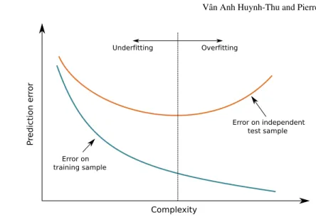
k=1 L(yk,f(xk)). (4)As the training error is calculated on the same samples that were used to learn the predictive model, it typically underestimates the generalisation error, as shown in Figure 1. The training error typically decreases when the complexity of the model is increased, i.e. when the model is allowed to fit more closely the training data. If the complexity is too high, the model may also fit the noise contained in the data and thus will have a poor generalisation performance. In this case, we say that the model
overfitsthe training data. On the other hand, if the model has a too low complexity, itunderfitsthe data and will also have a high generalisation error. Hence there is an optimal model complexity that leads to the minimal generalisation error.
For more details, the reader is invited to refer to general books about machine learning [25, 26].
3 Regression trees
A popular approach to the regression problem is the regression tree [27]. Figure 2 shows the structure of a tree. In this example, there are two input variablesX1and
X2, which are both continuous. Each interior node of the tree contains a test of the
type “Xi<c”, whereXi is one of the input variables andca threshold value, and
each terminal node (orleaf) contains a predicted value for the output variable. Given a new sample, for which we have observed values of the input variables, a prediction for the output is obtained by propagating the sample down the tree, until it reaches a leaf. The predicted output value is then the value at that leaf.
Complexity P redic tio n er ro r Overfitting Underfitting Error on independent test sample Error on training sample
Fig. 1 Overfitting and underfitting. The blue (resp. orange) curve plots, for varying levels of com-plexity of the predictive model, the average value of the loss function over the instances of the learning sample (resp. of an independent test sample). Overfitting occurs when the model is too complex and underfitting occurs when the model is not complex enough.
Fig. 2 Example of a regres-sion tree. Each interior node of a tree is a test on one input variable and each terminal node contains a predicted value for the output variable.
0.2587 0.1453 0.5412 x1 < 0.4 x2 < 1.7 yes no yes no
3.1 Learning a regression tree
Using a learning sampleLS, the goal of a tree-based method is to identify the tree that minimises the training error in Equation (4). A brute-force approach would con-sist in enumerating all the possible trees. This approach is however intractable and for this reason tree-based methods are rather based on greedy algorithms. A regres-sion tree is typically constructed top-down, starting from a root node corresponding to the whole learning sample. The idea is then to recursively split the learning
sam-ple with binary tests on the values of the input variables, trying to reduce as much as possible the variance of the output variable in the resulting subsets of samples. At each interior nodeN , the best test “Xi<c” is chosen, i.e. the variableXiand the
threshold valuecthat maximise:
I(N ) =#S.VarY(S)−#St.VarY(St)−#Sf.VarY(Sf), (5)
whereSdenotes the set of samples ofLSthat reach nodeN ,St(resp.Sf) denotes
its subset for which the test is true (resp. false), # denotes the cardinality of a set of samples, and VarY(·)is the variance of the output in a subsample. The samples ofS
are then split into two subsamples following the optimal test and the same procedure is applied on each of these subsamples. A node becomes a terminal node if the vari-ance of the output variable, computed over the samples reaching that node, is equal to zero. Each terminal node contains a predicted value for the output, corresponding to the mean value of the output taken over the samples that reach that node.
However, a fully grown tree typically overfits the training data. Overfitting can be avoided bypruning the tree, i.e. by removing some of its subtrees. Two types of pruning exist: pre-pruning and post-pruning. In a pre-pruning procedure, a node becomes a terminal node instead of a test node if it meets a given criterion, such as: • The number of samples reaching the node is below a thresholdNmin;
• The variance of the output variable, over the samples reaching the node, is below a threshold Varmin;
• The optimal test is not statistically significant, according to some statistical test. On the other side, the post-pruning procedure consists in fully developing a first tree
T1from the learning sample and then computing a sequence of trees{T2,T3, . . .}
such thatTi is a pruned version ofTi−1. The prediction error of each tree is then
calculated on an independent set of samples and the tree that leads to the lowest prediction error is selected. The main drawback of the post-pruning procedure is that an independent set of samples is needed, while the main drawback of pre-pruning is that the optimal value of the parameter related to the chosen stop-splitting criterion (Nmin, Varmin, the significance level) is dependent on the considered problem.
Besides pruning, ensemble methods constitute another way of avoiding overfit-ting. These methods are described in the following section.
3.2 Ensemble methods
Single regression trees are usually very much improved by ensemble methods, which average the predictions of several trees. The goal of ensemble methods is to use diversified models to reduce the overfitting of a learning algorithm. In the case of a tree, the overfitting comes mostly from the choices, made at each split node, of the input variable and the threshold value used for the test. Amongst the most widely used tree-based ensemble methods are methods that rely on
randomi-sation to generate diversity among the different models. These methods are Bagging [28], Random forest [29], and Extra-Trees [30].
Bagging
In the Bagging (for “Bootstrap AGGregatING”) algorithm, each tree of the ensem-ble is built from a bootstrap replica, i.e. a set of samples obtained by N random samplings with replacement in the original learning sample. The choices of the variable and of the threshold at each test node are thus implicitly randomised via the bootstrap sampling.
Random forest
This method adds an extra level of randomisation compared to the Bagging. In a Random forest ensemble, each tree is built from a bootstrap sample of the original learning sample and at each test node,K variables are selected at random (with-out replacement) among all the input variables before determining the best split. WhenKis set to the total number of input variables, the Random forest algorithm is equivalent to Bagging.
Extra-Trees
In the Extra-Trees (for “EXTremely RAndomised Trees”) method, each tree is built from the original learning sample but at each test node, the best split is determined amongKrandom splits, each determined by randomly selecting one input variable (without replacement) and a threshold value (chosen uniformly between the mini-mum and maximini-mum values of the input variable in the local subset of samples).
3.3 Parameters
Tree-based (ensemble) methods have several parameters whose values must be set by the user:
• The parameters related to the chosen stop-splitting criterion, such asNmin, the
minimal number of samples that a leaf node must contain. Increasing the value ofNmin results in smaller trees and hence models with a higher bias (i.e. more
prone to underfitting) and a lower variance (i.e. less prone to overfitting). Its optimal value depends on the level of noise contained in the learning sample. The noisier the data, the higher the optimal value ofNmin. Usually,Nminis fixed
• K, the number of input variables that are randomly chosen at each node of a tree. This parameter thus determines the level of randomisation of the trees. A smaller value ofKresults in more randomised trees. The optimal value ofKis problem-dependent, butK=√mandK=m, wheremis the number of input variables, are usually good default values [30].
• T, the number of trees in an ensemble. It can be shown that the higher the number of trees, the lower the generalisation error [29, 3]. Therefore, the chosen value of
T is a compromise between model accuracy and computing times.
3.4 Variable importance measures
One interesting characteristic of tree-based methods is the possibility to compute from a tree an importance score for each input variable. This score measures the relevance of a variable for the prediction of the output. In the case of regression, an importance measure that can be used is based on the reduction of the variance of the output at each test nodeN , i.e.I(N )as defined in Equation (5). For a single tree, the overall importancewiof one variableXiis then computed by summing the
I(N)values of all the tree nodes whereXiis used to split:
wi= p
∑
k=1
I(Nk)1Nk(Xi), (6)
wherepis the number of test nodes in the tree andNk denotes thek-th test node.
1Nk(Xi)is a function that is equal to one ifXiis the variable selected at nodeNkand
zero otherwise. The features that are not selected at all thus obtain an importance value of zero and those that are selected close to the root node of the tree typically obtain high scores. Variable importance measures can be easily extended to ensem-bles, simply by averaging importance scores over all the trees of the ensemble. The resulting importance measure is then even more reliable because of the variance reduction effect resulting from this averaging.
In the context of the Random forest method, an alternative procedure was pro-posed to compute the importance of a variable [29]. For each tree that was learned, this procedure consists in computing the prediction accuracy of the tree on the out-of-bag samples (i.e. the training instances that were not present in the bootstrap sample used to build the tree), before and after randomly permuting the values of the corresponding variable in these samples. The reduction of the tree accuracy that is obtained after the permutation is then computed, and the importance of the vari-able is given by the average accuracy reduction over all the trees of the ensemble. While this procedure has some advantages with respect to the variance reduction-based measure [31], it gives in most practical applications very similar results while being much more computationally demanding. Furthermore, it does not extend to methods that do not consider bootstrap sampling, like the Extra-Trees.
4 Tree-based approaches for gene network inference
This section presents several approaches based on decision tree algorithms, that were developed for the unsupervised inference of GRNs. In particular, we start by describing in detail the state-of-the-art GENIE3 approach.
4.1 GENIE3
GENIE3, for “GEne Network Inference with Ensemble of trees”, uses ensembles of regression trees to infer GRNs from steady-state expression data. (Many people think that the digit 3 in the acronym GENIE3 indicates a third version of the algo-rithm. This is however not the case. The presence of the digit 3 is actually due to the fact that the word “three” sounds exactly like the word “tree”, when pronounced with a (strong) French accent.)
In what follows, we define an expression dataset from which to infer the network as a collection ofNmeasurements:
D={x1,x2, . . . ,xN}, (7)
wherexk∈RG,k=1, . . . ,Nis the vector of expression values ofGgenes in thek-th experiment:
xk= (x1k,x2k, . . . ,xGk)
>.
The goal of GENIE3 is to exploit the expression dataset D to assign weights
wi,j > 0,(i,j=1, . . . ,G)to putative regulatory links from any genegito any gene
gj, with the aim of yielding larger values for weights that correspond to actual
regu-latory interactions. GENIE3 returns directed and unsigned edges, which means that
wi,jcan take a different value thanwj,i, and whengiis connected togj, the former
can be either an activator or a repressor of the latter.
To solve the network inference problem, GENIE3 decomposes the problem of recovering a network ofGgenes intoGdifferent subproblems, where each of these subproblems consists in identifying the regulators of one of the genes of the net-work. The method makes the assumption that the expression of each gene in a given condition is a function of the expression of the other genes in the same condition (plus some random noise). Denoting byx−kj the vector containing the expression values in thek-th experiment of all the genes except genegj:
x−kj= (x1k, . . . ,xkj−1,xkj+1, . . . ,xGk)>,
we can write:
xkj=fj(x
−j
k ) +εk,∀k, (8)
whereεkis a random noise with zero mean (conditionally tox
−j
k ). GENIE3 further
genes that are direct regulators ofgj, i.e. genes that are directly connected togjin
the targeted network. Recovering the regulatory links pointing to the target genegj
thus amounts to finding those genes whose expression is predictive of the expression ofgj. In machine learning terminology, this can be considered afeature selection
problem (in regression) for which many solutions can be found in the literature. The solution that is used by GENIE3 exploits the variable importance scores derived from tree ensemble models.
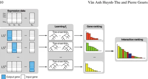
The GENIE3 procedure is illustrated in Figure 3 and works as follows: • For j= 1 toG:
– Generate the learning sample of input-output pairs for genegj:
LSj={(x−kj,xkj),k=1, . . . ,N}. (9)
– Learn an ensemble of trees fromLSjusing the Random forest or Extra-Trees algorithm.
– From the learned tree model, compute variable importance scoreswi,jfor all
the genesgi(exceptgjitself). These importance scores are computed as sums
of variance reductions (Equation (6)).
• Usewi,jas weight for the regulatory link directed fromgitogj.
Note that in GENIE3, it is possible – and even advisable – to restrict the set of can-didate regulators to a subset of the genes only (rather than using all theGgenes as candidate regulators). This can be useful when we know which genes are transcrip-tion factors for example. In that case, the learning sampleLSj is constructed with only those transcription factors as input genes.
4.1.1 Output normalisation
In the GENIE3 procedure, each tree-based model yields a separate ranking of the genes as potential regulators of a target gene gj, derived from importance scores wi,j. It can be shown that the sum of the importance scores of all the input variables
for a tree is equal to the total variance of the output variable explained by the tree, which in the case of unpruned trees (as they are in the case of tree ensembles) is usually very close to the initial total variance of the output:
∑
i6=j
wi,j≈NVarj(LS0j), (10)
whereLS0j is the learning sample from which the tree was built (i.e. LSj in the case of the Extra-Trees method and a bootstrap sample in the case of the Bagging and Random forest methods) and Varj(LS0j)is the variance of the target genegj
estimated in the corresponding learning sample. As a consequence, if the regulatory links are simply ranked according to the weightswi,j, this is likely to introduce a
Tree ensemble1 Tree ensemble2 Tree ensembleG Expressiondata ... ...
Output gene Input gene
Generanking Interactionranking ... ... Learningfj ... ... ... Exp1 Exp2 Exp3 ExpN ... ... ... g1 g2 g3 gG LS1 LS2 LSG
Fig. 3 GENIE3 procedure. For each genegj,j=1, . . . ,G, a learning sampleLSjis generated with the expression levels ofgjas output values and the expression levels of all the other genes as input values. An ensemble of trees is learned fromLSjand a variable importance scorewi,jis computed for each input genegi. The scorewi,jis then used as weight for the regulatory link directed from gitogj. Figure reproduced from [4].
they are directed towards highly variable genes. To avoid this bias, the expression of the target genegjis normalised to have a unit variance in the learning sampleLSj,
before applying the tree-based ensemble method:
xj← x
j
σj
,∀j, (11)
wherexj∈
RN is the vector of expression levels ofgjin theNexperiments andσj denotes its standard deviation. This normalisation indeed implies that the different weights inferred from different models predicting the different gene expressions are comparable.
4.1.2 Software availability
Python, MATLAB and R implementations of GENIE3, as well as tutorials explain-ing how to run them, are available from:
http://www.montefiore.ulg.ac.be/˜huynh-thu/GENIE3.html
4.1.3 Computational complexity
The computational complexity of the Random forest and Extra-Trees algorithms is on the order ofO(T KNlogN), where T is the number of trees,N is the learning sample size, andKis the number of randomly selected genes at each node of a tree.
GENIE3’s complexity is thus on the order ofO(GT KNlogN)since it requires to build an ensemble of trees for each of theGgenes. The complexity of the whole procedure is thus log linear with respect to the number of measurements and, at worst, quadratic with respect to the number of genes (whenK=G−1).
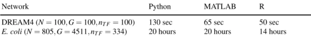
To give an idea of computing times, Table 1 shows the times needed for GENIE3 to infer one network of the DREAM4Multifactorialchallenge (100 experiments and 100 genes) and theE. colinetwork of the DREAM5 challenge (805 experiments and 4511 genes, among which 334 known transcription factors). In each case, GENIE3 was run with Random forest,T =1000 trees per ensemble andK = √nT F, where nT Fis the number of candidate regulators (i.e.nT F =100 for DREAM4 andnT F=
334 for E. coli). These computing times were measured on a 16GB RAM, Intel Xeon E5520 2.27 GHz computer.
Table 1 Running times of the different GENIE3 implementations
Network Python MATLAB R
DREAM4 (N=100,G=100,nT F=100) 130 sec 65 sec 50 sec
E. coli(N=805,G=4511,nT F=334) 20 hours 20 hours 14 hours
N: number of samples,G: number of genes,nT F: number of transcription factors.
Note that if needed, the GENIE3 algorithm can be easily parallelised as theG
feature selection problems, as well as the different trees in an ensemble, are inde-pendent of each other.
4.1.4 Parameter analysis
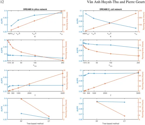
Figure 4 shows the performances and running times of GENIE3, for two networks of the DREAM5 challenge (an artificialIn silico network and a realE. coli net-work), when varying the values of the different parameters of GENIE3. The perfor-mances were measured using the area under the precision-recall curve (AUPR) met-ric, which assesses the quality of the ranking of interactions returned by a method. A perfect ranking, where all the true interactions are ranked at the top, yields an AUPR equal to 1, while a random ranking returns an AUPR equal to the proportion of true interactions among all the possible interactions (which is typically very small, since regulatory networks are very sparse).
Clearly, the parameter with the highest impact isK, i.e. the number of randomly selected candidate regulators at each tree node. Its optimal value is very dataset-dependent: increasing the value of K improves the predictions (i.e. the AUPR is increased) for theIn siliconetwork, while the opposite is observed on theE. coli
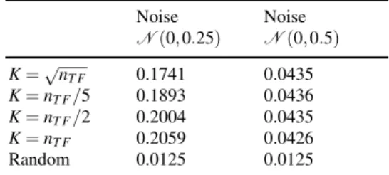
network. This difference between the two networks can probably be explained by the fact that theE. colidata contains more noise than the artificial data. We thus checked how the performance of GENIE3 varies when adding further noise to the artificial data, in the form of a Gaussian noise∼N(0,0.25)orN(0,0.5)(Table 2).
sqrt(nTF) nTF/5 nTF/2 nTF K 0.25 0.3 0.35 0.4 AUPR 0 20 40 60
Running time (hours)
DREAM5 In silico network
sqrt(nTF) nTF/5 nTF/2 nTF K 0.06 0.07 0.08 0.09 0.1 AUPR 0 100 200 300
Running time (hours)
DREAM5 E. coli network
1510 20 50 100 200 nmin 0.25 0.3 0.35 0.4 AUPR 2 3 4 5
Running time (hours)
1510 20 50 100 200 nmin 0.06 0.07 0.08 0.09 0.1 AUPR 0 5 10 15 20
Running time (hours)
100 500 1000 2000 5000 T 0.25 0.3 0.35 0.4 AUPR 0 10 20 30
Running time (hours)
100 500 1000 2000 5000 T 0.06 0.07 0.08 0.09 0.1 AUPR 0 20 40 60 80
Running time (hours)
RF ET Tree-based method 0.25 0.3 0.35 0.4 AUPR 2 3 4 5
Running time (hours)
RF ET Tree-based method 0.06 0.07 0.08 0.09 0.1 AUPR 6 8 10 12 14 16
Running time (hours)
Fig. 4 AUPRs (blue circles) and running times (orange triangles) of GENIE3, when varying the values of the parametersK(number of randomly chosen candidate regulators at each split node of a tree),nmin(minimum number of samples at a leaf) andT(number of trees per ensemble), and when using either Random forest (RF) or Extra-Trees (ET) as tree-based algorithm. When varying the values of one parameter, the values of the remaining parameters were set to their default values. The default values are:K=√nT F, wherenT F is the number of transcription factors,nmin=1, T=1000 and the tree-based method is the Random forest algorithm. The results shown in this figure were obtained by using the R implementation of GENIE3.In silicodataset: 805 samples, 1643 genes, 195 transcription factors.E. colidataset: 805 samples, 4511 genes, 334 transcription factors.
As expected, the predictions are worse when noise is added, for all the values ofK. In the presence of a high amount of noise, increasingKfrom nT F
2 tonT F results in
a (slightly) lower AUPR, a result closer to what is observed for theE. colinetwork. This could be explained by the fact that decreasing the value ofKresults in predic-tive tree-based models that overfit less the data and that are therefore more robust to the noise.
The other parameters of GENIE3 have only a minor impact on the performances (Figure 4). In terms of AUPR, the best value ofnmin, i.e. the minimum number of
samples at a leaf, is 1. Increasingnminallows to save some computational time, at
only a small cost in terms of performances. Regarding the numberT of trees per ensemble, we observe that 500 trees already allows to obtain good performances. Further increasing T only results in more computational time, without improving
Table 2 AUPRs of GENIE3 for the DREAM5In siliconetwork, when noise is added to the data Noise N(0,0.25) Noise N(0,0.5) K=√nT F 0.1741 0.0435 K=nT F/5 0.1893 0.0436 K=nT F/2 0.2004 0.0435 K=nT F 0.2059 0.0426 Random 0.0125 0.0125
the AUPR. Finally, the Extra-Trees algorithm has slightly less good performances than Random forest, but is more computationally efficient.
4.2 Extensions of GENIE3
Several methods for GRN inference building on GENIE3 have been developed. The purpose of this section is to give a brief overview of these methods. For more details, the reader can refer to the original articles (referenced in the following subsections).
4.2.1 Analysis of time series data
dynGENIE3 (for “dynamical GENIE3”) is a variant of GENIE3 that was developed for the analysis of time series of expression data [32]. dynGENIE3 assumes that the expression levelxjof genegjis modelled through the following ordinary differential
equation (ODE):
dxj(t)
dt =−αjxj(t) +fj(x(t)), (12)
wherex(t)is the vector containing the expressions of all theGgenes at timetand αj is a parameter specifying the decay rate ofxj. In this ODE, it is assumed that
the transcription rate ofxjis a (potentially non-linear) function fjof the expression
levels of theGgenes. Like in GENIE3, this function fj is learned in the form of
an ensemble of regression trees and the regulators ofgjare then identified by
com-puting the variable importance scores derived from the tree model. dynGENIE3 is therefore a semi-parametric approach, as the temporal evolution of each gene ex-pression is modelled with a formal ODE while the transcription function in each ODE is learned in the form of a non-parametric (tree-based) model.
Given the observation time pointst1,t2, . . . ,tT, the ODE (12) has the following
finite approximation:
xj(tk+1)−xj(tk)
tk+1−tk +αjxj(tk) =fj(x(tk)),
and the function fjcan thus be learned using the following learning sample:
LSj={(x(tk),
xj(tk+1)−xj(tk) tk+1−tk
+αjxj(tk)),k=1, . . . ,T−1}. (14)
The gene decay ratesαj inLSjare parameters that are fixed by the user. Their
values may be retrieved from the literature, since there exist many studies that ex-perimentally measure the mRNA decay rates in different organisms. However, when such information is not available, a data-driven approach can be used to estimate the αjvalue directly from the observed expressionsxjofgj. For example, a rough
es-timate ofαjcan be obtained by assuming an exponential decaye−αjt between the
highest and lowest values ofxj.
4.2.2 Analysis of genotype data
Two extensions of GENIE3 were proposed for the joint analysis of expression and genotype data [33]. It is assumed that we have at our disposal a dataset containing the expression levels ofGgenes measured inNindividuals, as well as the genotype value of one genetic marker for each of these genes in the sameNindividuals:
D={(x1,m1),(x2,m2), . . . ,(xN,mN)}, (15)
wherexk∈RG andmk∈ {0,1}G,k=1, . . . ,N are respectively the vectors of
ex-pression levels and genotype values of theGgenes in thek-th individual:
xk= (x1k,x2k, . . . ,xGk)>,
mk= (m1k,m2k, . . . ,mGk)
>. (16)
Note that it is supposed that each genetic marker can have two possible genotype values only (0 or 1), as it would be the case for homozygous individuals.
To exploit such data, the first procedure, called GENIE3-SG-joint, assumes that a unique model fjexplains the expression of a genegjin a given individual, knowing
the expression levels and the genotype values of the different genes:
xkj=fj(x
−j
k ,mk) +εk,∀k, (17)
whereεkis a random noise. In the second procedure, called GENIE3-SG-sep, it is
assumed that two different models fjxandfmj can both explain the expression ofgj,
either from the expression levels of the other genes, or from the genotype values: (
xkj=fxj(xk−j) +εk,∀k, xkj=fmj (mk) +εk0,∀k.
(18)
The functions fej and fmj are therefore respectively learned from two different learn-ing samples. Both GENIE3-SG-joint and GENIE3-SG-sep learn the different
func-tionsfjas ensembles of trees and compute for each candidate regulatorgitwo scores wxi,j andwmi,j, measuring respectively the importances of the expression and of the marker ofgiwhen predicting the expression ofgj. These two scores are then
aggre-gated, either by a sum or a product, to obtain a single weightwi,jfor the regulatory
link directed fromgitogj.
4.2.3 Analysis of single-cell data
GENIE3 is used as such in two frameworks that were developed for the inference of GRNs from single-cell transcriptomic data.
The framework developed by Oconeet al.uses GENIE3 to obtain a prior GRN, which is then refined using an ODE-based approach [34]. The whole procedure allows to identify the GRN as well as the parameters of the ODEs that are used to model the gene expression dynamics.
In the SCENIC framework [35], GENIE3 is used in a first step to identify co-expression modules, i.e. groups of genes that are regulated by the same transcription factor. In a second step, a motif enrichment analysis is performed for each module, and only the modules such that the target genes show an enrichment of a motif of the corresponding transcription factor are retained. The activity of each module in each cell is then evaluated using the single-cell expression data and the activity levels of the different modules are used to perform cell clustering.
4.2.4 Exploitation of prior knowledge
The iRafNet method [36] allows to take into account prior information that we have about the network, in the form of prior weights associated with the different network edges. In the original article introducing iRafNet, the prior weights are obtained from diverse types of data, such as protein-protein interaction data or knockout data. To exploit the prior weights, iRafNet uses the same framework as GENIE3, but with a modified version of the Random forest algorithm. At each tree node, instead of randomly sampling K input variables according to a uniform distribution, the
K variables are sampled with a bias that favours the variables with a higher prior weight.
4.2.5 Inference of context-specific networks
Let us assume that we have different expression datasets respectively related to dif-ferent contexts (e.g. difdif-ferent pathological conditions). One could then be interested in identifying a GRN that is specific to each of these contexts. To achieve such goal, one could apply a network inference algorithm like GENIE3 to each dataset. How-ever, when the contexts are related (e.g. different subclasses of a cancer), one can expect the different networks to have a lot of commonalities. In this case, approaches
that jointly analyse the different datasets will potentially yield better performances, as they will assign higher weights to regulatory links that are active in a higher number of contexts. Many of such joint approaches are based on Gaussian graph-ical models (see e.g. [37–39]). An approach based on trees, called JRF (for “Joint Random Forest”) [40], has also been proposed. GivenDdatasets, JRF consists, for each target gene, in simultaneously learningDtree models. When learningD regres-sion trees in parallel, the idea is to select the same input variable at the same node position in theDdifferent trees. More specifically, for a given input variablegi, let cdi be the threshold value that yields the best split at test node N in thed-th tree
(d=1, . . . ,D).cdi is thus the threshold value that maximises the variance reduction
Iid(N), as defined in Equation (5), among all the possible threshold values forgi.
JRF then selects, at nodeN in all theDtrees, the input variablegi∗ that maximises: gi∗=arg max i D
∑
d=1 Iid(N ) Nd , (19)whereNd is the number of samples in thed-th dataset. The importance score of
a candidate regulator gi in thed-th context is then the sum of output variance
re-ductions (as defined in Equation (6)), computed by propagating the samples of the
d-th dataset in thed-th tree model. By selecting, for a given target gene, the same candidate regulators in theDtree models, JRF enforces the similarity between the inferred networks. However, since the importance score ofgiin thed-th context is
computed by using the samples that are related to this context, JRF also allows to identify regulatory links that are active in only one or a few contexts. Note that when there is only one context, JRF is equivalent to GENIE3.
4.3 Other tree-based approaches
Besides GENIE3, other tree-based approaches have been proposed for the unsuper-vised inference of GRNs, which use different types of trees in different frameworks. In [41], networks are reconstructed by learning a single classification tree for each target gene, predicting the state of the gene (up- or down-regulated) from the ex-pression levels of the other genes. In [42], Segalet al.propose a method that par-titions the genes intomodules, such that genes in the same module have the same regulators and the same regulatory model. The regulatory model of each module is represented by one probabilistic regression tree (where each leaf is associated with a probabilistic distribution of the output variable). Inspired by the work of Segal
al., the LeMoNe algorithm [43] also learns module networks, where the regulatory model for each module is in the form of an ensemble offuzzydecision trees. In [44] M5’ model trees are used, i.e. regression trees with linear models at the leaves. In [45], networks are reconstructed by fitting a dynamical model of the gene expres-sions, where one of the terms of the model is learned in the form of an ensemble of decision trees. Tree-based methods were also used to model expression data jointly
with other types of data, such as motif counts in the promoter regions of the gene or transcription factor-binding data [46–49]. Another example is [50], which extends the module network procedure to exploit both expression and genotype data.
5 Discussion
In this chapter, we presented GENIE3 and other tree-based approaches, that were developed for the inference of gene regulatory networks from expression data. The main advantages of GENIE3 are its non-parametric nature, its ability to detect mul-tivariate interacting effects between candidate regulators and the fact that it has very few parameters. However, like any method, GENIE3 also has its own limitations and could thus be improved along several directions, discussed below.
A first limitation of GENIE3 is that it provides a ranking of the putative reg-ulatory links, rather than a network topology. Since tree-based importance scores are not interpretable from a statistical point of view, choosing a threshold value to distinguish present and absent edges is not a trivial task. Several methods were pro-posed for addressing the problem of selecting, from tree-based importance scores, the input variables that are relevant for output prediction [51, 52]. These methods could in principle be applied in the context of GENIE3 in order to select the regu-lators of each target gene. However, most of them are based on multiple – say 1000 – reruns of the tree-based algorithm. If one wishes to incorporate such feature se-lection approaches into GENIE3, one would need to learn 1000×Gensembles of trees, whereGis the number of genes, which would be impractical for a large value of G. Another property of these methods is that they are designed to identify the
maximalsubset of relevant variables, i.e. all the variables that convey at least some information about the output. For that reason, these methods are not appropriate for the network inference problem. Even if there is no direct edge from genegito gene gj in the true network, the expression ofgican still be predictive of the expression
of gj, through one or several other genes (e.g. gi regulates some gene gk, which
in turn regulates gj). In conclusion, each gene of the network is indirectly
regu-lated by (almost) all the other genes, but most of these indirect edges are considered false positives since they are not part of the true network. To avoid the inclusion of such indirect effects, one would need a feature selection method able to determine aminimalsubset of variables that convey all the information about an output (and thus make all the other variables conditionally irrelevant). An optimal treatment of this problem would probably require to adopt a more global approach that exploits jointly theGindividual rankings related to the different target genes respectively.
GENIE3 could also be improved on the way the variable importance scores are normalised. Given the current normalisation (Equation (11)), the scores of all the pu-tative edges directed towards a given target gene sum up to one. As a consequence, the importance scores that are derived from different tree models are not entirely comparable. For example, let us assume that geneg1has a single regulatorg2, and
will assign a score of 1 to the edgeg2→g1, but a score of only 0.5 tog4→g3and
g5→g3. An optimal way of normalising the importance score is thus still needed at
this stage.
So far, GENIE3 has only been evaluated in an empirical way. It would however be interesting to better characterise the method – in particular the tree-based im-portance scores used within – from a theoretical point of view. This would actually constitute an important contribution in the machine learning field, as there has been very few works focusing on the theoretical analysis of the importance measures derived from tree ensembles [53–55].
Despite the good scalability of GENIE3 with respect to some families of methods (such as methods based on differential equations or Bayesian methods), a substantial amount of time is still needed to reconstruct a large network (e.g. it takes 20 hours to reconstruct theE. colinetwork from 805 samples, see Table 1). With the recent developments in single-cell RNA-seq technologies, datasets with a size of the order of 100K cells are becoming available. Speeding up the GENIE3 algorithm would be necessary if one wishes to apply it on such large datasets.
Acknowledgements VAHT is a Post-doctoral Fellow of the F.R.S.-FNRS.
References
[1] Geurts P, Irrthum A, Wehenkel L (2009) Supervised learning with deci-sion tree-based methods in computational and systems biology. Mol Biosyst 5(12):1593–605
[2] Boulesteix AL, Janitza S, Kruppa J, K¨onig IR (2012) Overview of random forest methodology and practical guidance with emphasis on computational biology and bioinformatics. Wiley Interdisciplinary Reviews: Data Mining and Knowledge Discovery 2(6):493–507
[3] Biau G, Scornet E (2016) A random forest guided tour. TEST 25(2):197–227 [4] Huynh-Thu VA, Irrthum A, Wehenkel L, Geurts P (2010) Inferring
regula-tory networks from expression data using tree-based methods. PLoS ONE 5(9):e12,776
[5] Marbach D, Costello JC, K¨uffner R, Vega N, Prill RJ, Camacho DM, Al-lison KR, the DREAM5 Consortium, Kellis M, Collins JJ, Stolovitzky G (2012) Wisdom of crowds for robust gene network inference. Nature Meth-ods 9(8):796–804
[6] Omranian N, Eloundou-Mbebi JMO, Mueller-Roeber B, Nikoloski Z (2016) Gene regulatory network inference using fused lasso on multiple data sets. Scientific Reports 6:20,533
[7] Kiani NA, Zenil H, Olczak J, Tegn´er J (2016) Evaluating network inference methods in terms of their ability to preserve the topology and complexity of genetic networks. Seminars in Cell & Developmental Biology 51:44 – 52
[8] Bellot P, Olsen C, Salembier P, Oliveras-Verg´es A, Meyer PE (2015) Net-Benchmark: a bioconductor package for reproducible benchmarks of gene reg-ulatory network inference. BMC Bioinformatics 16:312
[9] Maetschke SR, Madhamshettiwar PB, Davis MJ, Ragan MA (2014) Super-vised, semi-supervised and unsupervised inference of gene regulatory net-works. Briefings in Bioinformatics 15(2):195–211
[10] Zhang X, Liu K, Liu ZP, Duval B, Richer JM, Zhao XM, Hao JK, Chen L (2013) NARROMI: a noise and redundancy reduction technique improves ac-curacy of gene regulatory network inference. Bioinformatics 29(1):106–113 [11] Feizi S, Marbach D, M´edard M, Kellis M (2013) Network deconvolution
as a general method to distinguish direct dependencies in networks. Nature Biotechnology 31:726–733
[12] Madhamshettiwar PB, Maetschke SR, Davis MJ, Reverter A, Ragan MA (2012) Gene regulatory network inference: evaluation and application to ovar-ian cancer allows the prioritization of drug targets. Genome Medicine 4(5):41 [13] Qi J, Michoel T (2012) Context-specific transcriptional regulatory network in-ference from global gene expression maps using double two-way t-tests. Bioin-formatics 28(18):2325–2332
[14] Imam S, Noguera DR, Donohue TJ (2015) An integrated approach to recon-structing genome-scale transcriptional regulatory networks. PLoS Computa-tional Biology 11(2):e1004,103
[15] Arrieta-Ortiz ML, Hafemeister C, Bate AR, Chu T, Greenfield A, Shuster B, Barry SN, Gallitto M, Liu B, Kacmarczyk T, Santoriello F, Chen J, Rodrigues CD, Sato T, Rudner DZ, Driks A, Bonneau R, Eichenberger P (2015) An experimentally supported model of the bacillus subtilis global transcriptional regulatory network. Molecular Systems Biology 11(11)
[16] Carrera J, Estrela R, Luo J, Rai N, Tsoukalas A, Tagkopoulos I (2014) An integrative, multi-scale, genome-wide model reveals the phenotypic landscape of escherichia coli. Molecular Systems Biology 10(7)
[17] Sabaghian E, Drebert Z, Inz´e D, Saeys Y (2015) An integrated network of
Arabidopsisgrowth regulators and its use for gene prioritization. Scientific Reports 5:17,617
[18] Taylor-Teeples M, Lin L, de Lucas M, Turco G, Toal TW, Gaudinier A, Young NF, Trabucco GM, Veling MT, Lamothe R, Handakumbura PP, Xiong G, Wang C, Corwin J, Tsoukalas A, Zhang L, Ware D, Pauly M, Kliebenstein DJ, De-hesh K, Tagkopoulos I, Breton G, Pruneda-Paz JL, Ahnert SE, Kay SA, Hazen SP, Brady SM (2015) AnArabidopsisgene regulatory network for secondary cell wall synthesis. Nature 517(7536):571–575
[19] Marchand G, Huynh-Thu VA, Kane N, Arribat S, Var`es D, Rengel D, Balz-ergue S, Rieseberg L, Vincourt P, Geurts P, Vignes M, Langlade NB (2014) Bridging physiological and evolutionary time-scales in a gene regulatory net-work. New Phytologist 203(2):685–696
[20] Potier D, Davie K, Hulselmans G, NavalSanchez M, Haagen L, Huynh-Thu V, Koldere D, Celik A, Geurts P, Christiaens V, Aerts S (2014) Mapping gene
reg-ulatory networks inDrosophilaeye development by large-scale transcriptome perturbations and motif inference. Cell Reports 9(6):2290–2303
[21] Jo J, Hwang S, Kim HJ, Hong S, Lee JE, Lee SG, Baek A, Han H, Lee JI, Lee I, Lee DR (2016) An integrated systems biology approach identifies positive cofactor 4 as a factor that increases reprogramming efficiency. Nucleic Acids Research 44(3):1203–1215
[22] Acquaah-Mensah GK, Taylor RC (2016) Brain in situ hybridization maps as a source for reverse-engineering transcriptional regulatory networks: Alzheimer’s disease insights. Gene 586(1):77 – 86
[23] Verfaillie A, Imrichova H, Atak ZK, Dewaele M, Rambow F, Hulselmans G, Christiaens V, Svetlichnyy D, Luciani F, Van den Mooter L, Claerhout S, Fiers M, Journe F, Ghanem GE, Herrmann C, Halder G, Marine JC, Aerts S (2015) Decoding the regulatory landscape of melanoma reveals teads as regulators of the invasive cell state. Nature Communications 6:6683
[24] Ko JH, Gu W, Lim I, Zhou T, Bang H (2014) Expression profiling of mitochon-drial voltage-dependent anion channel-1 associated genes predicts recurrence-free survival in human carcinomas. PLoS ONE 9(10):e110,094
[25] Hastie T, Tibshirani R, Friedman J (2009) The elements of statistical learning: data mining, inference and prediction, 2nd edn. Springer
[26] Bishop CM (2006) Pattern Recognition and Machine Learning. Springer [27] Breiman L, Friedman JH, Olsen RA, Stone CJ (1984) Classification and
Re-gression Trees. Wadsworth International (California)
[28] Breiman L (1996) Bagging predictors. Machine Learning 24(2):123–140 [29] Breiman L (2001) Random forests. Machine Learning 45(1):5–32
[30] Geurts P, Ernst D, Wehenkel L (2006) Extremely randomized trees. Machine Learning 36(1):3–42
[31] Strobl C, Boulesteix AL, Zeileis A, Horthorn T (2007) Bias in random for-est variable importance measures: Illustrations, sources and a solution. BMC Bioinformatics 8:25
[32] Huynh-Thu VA, Geurts P (2018) dynGENIE3: dynamical GENIE3 for the in-ference of gene networks from time series expression data. Scientific Reports 8(1):3384
[33] Huynh-Thu VA, Wehenkel L, Geurts P (2013) Gene regulatory network infer-ence from systems genetics data using tree-based methods. In: de la Fuente A (ed) Gene Network Inference - Verification of Methods for Systems Genetics Data, Springer, pp 63–85
[34] Ocone A, Haghverdi L, Mueller NS, Theis FJ (2015) Reconstructing gene reg-ulatory dynamics from high-dimensional single-cell snapshot data. Bioinfor-matics 31(12):i89–i96
[35] Aibar S, Gonz´alez-Blas CB, Moerman T, Huynh-Thu VA, Imrichova H, Hulselmans G, Rambow F, Marine JC, Geurts P, Aerts J, van den Oord J, Atak ZK, Wouters J, Aerts S (2017) SCENIC: single-cell regulatory network infer-ence and clustering. Nature Methods 14:1083–1086
[36] Petralia F, Wang P, Yang J, Tu Z (2015) Integrative random forest for gene regulatory network inference. Bioinformatics 31(12):i197–i205
[37] Chiquet J, Grandvalet Y, Ambroise C (2011) Inferring multiple graphical structures. Statistics and Computing 21(4):537–553
[38] Mohan K, London P, Fazel M, Witten D, Lee SI (2014) Node-based learning of multiple gaussian graphical models. J Mach Learn Res 15(1):445–488 [39] Tian D, Gu Q, Ma J (2016) Identifying gene regulatory network rewiring using
latent differential graphical models. Nucleic Acids Research 44(17):e140 [40] Petralia F, Song WM, Tu Z, Wang P (2016) New Method for Joint Network
Analysis Reveals Common and Different Coexpression Patterns among Genes and Proteins in Breast Cancer. Journal of Proteome Research 15(3):743–754 [41] Soinov LA, Krestyaninova MA, Brazma A (2003) Towards reconstruction of
gene networks from expression data by supervised learning. Genome Biology 4(1):R6
[42] Segal E, Shapira M, Regev A, Pe’er D, Botstein D, Koller D, Friedman N (2003) Module networks: identifying regulatory modules and their condition-specific regulators from gene expression data. Nature Genetics 34:166–176 [43] Joshi A, De Smet R, Marchal K, Van de Peer Y, Michoel T (2009) Module
networks revisited: computational assessment and prioritization of model pre-dictions. Bioinformatics 25(4):490–496
[44] Nepomuceno-Chamorro IA, Aguilar-Ruiz JS, Riquelme JC (2010) Inferring gene regression networks with model trees. BMC Bioinformatics 11:517 [45] Huynh-Thu VA, Sanguinetti G (2015) Combining tree-based and
dynami-cal systems for the inference of gene regulatory networks. Bioinformatics 31(10):1614–1622
[46] Middendorf M, Kundaje A, Wiggins C, Freund Y, Leslie C (2004) Pre-dicting genetic regulatory response using classification. Bioinformatics 20(suppl 1):i232–i240
[47] Phuong TM, Lee D, Lee KH (2004) Regression trees for regulatory element identification. Bioinformatics 20(5):750–757
[48] Ruan J, Zhang W (2006) A bi-dimensional regression tree approach to the modeling of gene expression regulation. Bioinformatics 22(3):332–340 [49] Xiao Y, Segal MR (2009) Identification of yeast transcriptional regulation
networks using multivariate random forests. PLOS Computational Biology 5(6):e1000,414
[50] Lee SI, Pe’er D, Dudley AM, Church GM, Koller D (2006) Identify-ing regulatory mechanisms usIdentify-ing individual variation reveals key role for chromatin modification. Proceedings of the National Academy of Sciences 103(38):14,062–14,067
[51] Huynh-Thu VA, Saeys Y, Wehenkel L, Geurts P (2012) Statistical interpreta-tion of machine learning-based feature importance scores for biomarker dis-covery. Bioinformatics 28(13):1766–1774
[52] Degenhardt F, Seifert S, Szymczak S (2017) Evaluation of variable selection methods for random forests and omics data sets. Briefings in Bioinformatics p bbx124
[53] Ishwaran H (2007) Variable importance in binary regression trees and forests. Electron J Statist 1:519–537
[54] Louppe G, Wehenkel L, Sutera A, Geurts P (2013) Understanding variable im-portances in forests of randomized trees. In: Burges CJC, Bottou L, Welling M, Ghahramani Z, Weinberger KQ (eds) Advances in Neural Information Pro-cessing Systems 26, Curran Associates, Inc., pp 431–439
[55] Sutera A, Louppe G, Huynh-Thu VA, Wehenkel L, Geurts P (2016) Context-dependent feature analysis with random forests. In: Proceedings of the Thirty-Second Conference on Uncertainty in Artificial Intelligence, AUAI Press, UAI’16, pp 716–725