Using SSD-Assisted Scalable Elasticity to
Improve Inline Data Deduplication Storage
Systems
Yufeng Wang, Zhengyu Yang, Ningfang Mi, Chiu C Tan
Abstract—Elasticity is the ability to scale computing resources such as memory on-demand, and is one of the main advantages of utilizing cloud computing services. With the increasing popularity of cloud based storage, it is natural that more deduplication based storage systems will be migrated to the cloud. Existing deduplication systems, however, do not adequately take advantage of elasticity. In this paper, we first present a SSD (Solid State Drive)-based multi-tier storage architecture to improve caching capacity of current deduplication systems. With such an enhanced system, we attempt to optimize deduplication approaches to achieve higher memory utilization efficiency. Then, we illustrate how to use elasticity to improve deduplication based systems, and propose EAD (elasticity aware deduplication), an indexing algorithm that uses the ability to dynamically increase memory and SSD resources to improve overall deduplication performance. Our experimental results indicate that EAD is able to detect more than 98% of all duplicate data, however only consumes less than 5% of expected memory space. Meanwhile, it claims four times of deduplication efficiency than the state-of-art sampling technique while costs less than half of the amount of memory. We further proposed an online scaling up algorithm that takes advantage of the elasticity of cloud computing to dynamically trigger scaling up operation. Our algorithm also offers a complete guideline for its large scale deployment. The experimental results show that our design save at least 74% of overall I/O access cost compared to the traditional design.
Index Terms—Deduplication, Flash-based SSD, Scaling Up, Migration, Cloud Computing, Cloud Storage Systems, Fusion Disk
F
1
I
NTRODUCTIONData deduplication is a technique used to reduce storage and transmission overhead by identifying and eliminating redundant data segments. It splits files into multiple data chunks that are each uniquely identified by a fingerprint (FP) that usually is a hash signature of the data chunk. The redundant data chunks in a file are replaced by the pointers. Data deduplication has been an essential and critical component in cloud backup, synchronization and archiving storage systems. It not only reduces the storage space requirements, but also improves the throughput of the backup and archiving systems by eliminating the network transmis-sion of redundant data, as well as reduces the energy consumption by deploying fewer disks. Therefore, data deduplication plays an important role in existing storage systems [1], and its importance will continue to grow as the amount of data increases (the growth of data is estimated to reach 35 zettabytes in the year 2020) in cloud backup, synchronization and archiving storage systems.
There are two types of deduplication systems: inline and offline. Clients in the former system first transmits • Yufeng Wang and Zhengyu Yang share equal credit for this paper.
• Yufeng Wang and Chiu C Tan are with Department of Computer and Information Sciences at Temple University.
• Zhengyu Yang and Ningfang Mi are with Department of Electrical and Computer Engineering at Northeastern University.
metadata to the server to detect duplications and only the new data is going to be sent to the server. While, clients in the latter system transfer all data to the server and then the server conducts the deduplication process. In this paper we use the inline deduplication system [2], [3]. However, in the inline deduplication system, with the ever increasing amount of new data, searching chunks’ existence in the huge dataset stored in the slow-access-speed disk (usually magnetic disk MD) is a time consuming process, which is the main bottleneck of deduplication implementations. To improve overall speed, the memory (RAM) is practically used to cache hot chunks’ metadata (e.g. index table). Unfortunately, deduplication systems currently need to scale to tens of terabytes to petabytes of data volume, the ever increas-ing amounts of new data will finally flush the existincreas-ing useful data cached in the memory, whose penalty beats the benefit brought from the performance gap between in-memory searching and disk lookups. Motivated by this disk I/O speed bottleneck issue, we start to solve it in three different directions:
Our first direction is to improve the performance of the cache system. Since we cannot easily increase RAM’s size and MD’s access speed with a low cost, a feasible way is to introduce an extra storage tier between RAM and MD. This storage tier should be faster than MD and cheaper than RAM. We find that NAND-flash based solid-state disks (SSDs) meet these two conditions and can be a good candidate for the “middle” storage. We thus adopt a three-tier caching system, consisting of RAM, SSD and
MD, to increase the speed for accessing huge dataset in the MD and enlarge the cache size for storing hot data. Our second direction is to best use the cache through downsampling algorithms. Since cache systems cannot be infinite large, we need to filter non-critical data out of the cache, and decide what to load from the MD to SSD and RAM. Existing research [4] [5] [6] in this area proposed different sampling algorithms to index more data using less memory. The key features of our solution is that our deduplication algorithm is compatible with current deduplication techniques such as sampling to take advantage of locality [5], [6], and content-based chunking [7]–[9].
Our last direction is to dynamically scale up the storage system during runtime. In real cases, due to customer’s high desired deduplication degree or special incoming data types that naturally have low dedupli-cation ratio (like videos and encrypted files), the in-sufficient RAM (including SSD) caching system will be eventually flushed by the incoming data stream. This issue cannot be thoroughly solved by the multi-tier caching system and downsampling algorithms. Fortu-nately, the key property of cloud computing – elasticity can be used to improve deduplication systems by allow-ing deduplication storage systems to dynamically adjust the amount of memory resources as needed to detect sufficient amount of duplicate data. In industrial envi-ronments, the flexibility and cost advantages of cloud computing providers such as Azure [10], Amazon [11], etc. make deploying new resources in the cloud during runtime as an possible option. Based on these facts, we then proposed an elasticity-aware deduplication (EAD) algorithm to dynamically assign new resources. EAD solves the two main problems in this topic – when to trigger the scaling up operation and how much new resources are “enough” for the future.
In summary, in this paper we design a multi-tier storage architecture to enhance the caching capacity of the deduplication system. We optimize the approach to claim higher RAM utilization efficiency and best use the caching system, by using downsampling-based algo-rithms. We finally propose an elasticity-aware dedupli-cation (EAD) algorithm that takes advantage of the elas-ticity of cloud computing to dynamically trigger scaling up operation. Furthermore, we also present a detailed analysis of our algorithm, as well as the evaluation using extensive experiments on real dataset.
The rest of the paper is organized as follows: Section 2 explores the background of the deduplication system bottleneck and approaches. Section 3 describes the detail of EAD design also including scaling up strategy and the storage hierarchy. Section 4 evaluates our solution, and Section 5 contains the related work. Section 6 draws conclusion of the paper.
2
B
ACKGROUNDThis section will discuss the background knowledges of deduplication, including its bottleneck, and further
explore some alternatives to improve deduplication per-formance.
2.1 Data Deduplication Basics
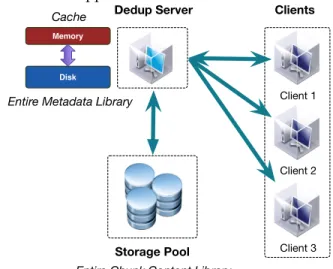
As shown in Figure 1, in a typical cloud-based dedu-plication system, there is a DedupServer taking charge of processing deduplication requests. The DedupServer itself does not store any chunk contents, but only keeps the entire metadata library in its disk which tracks the fingerprint of each chunk and its address in the storage pool. In addition, DedupServer’s disk memory caches the hot index table entries to accelerate the overall access speed. The basic deduplication process first dives the incoming data stream into (fixed/variable size) chunks, and segments (groups of chunks based on their local-ity). Next, duplicate chunks are then identified by their hash fingerprints (FP) calculated on their contents. The server then needs to lookup each chunk hash in an index it maintains for all chunks seen so far for that storage location (dataset) instance. If there is a match, the incoming chunk contains redundant data and can be deduplicated; if not, the (new) chunk needs to be added to the system and its hash and metadata need to be inserted into the index. Detailed algorithm is shown in Algorithm 1, where a memory-disk deduplication architecture is applied.
Client 1 Dedup Server Clients
Storage Pool Memory Disk Client 2 Client 3 Cache
Entire Metadata Library
Entire Chunk Content Library
Fig. 1:A typical cloud-based deduplication system 2.2 Understanding SSDs
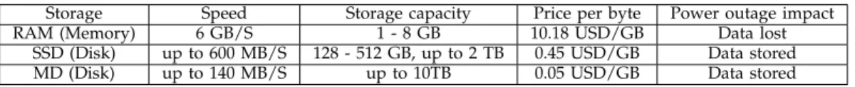
As discussed before, the slow-access-speed of disk is the bottleneck of a deduplication system. To address this issue, we consider to use SSDs as the “middle” storage tier between RAM and MD. Table 1 shows a comparison between RAM, SSD and MD. Specifically, flash-based SSDs have the following characteristics which help to improve efficiency of the deduplication design:
1) High access speed: Different from MDs, flash-based SSDs are made of silicon memory chips and have no moving parts. Thus both read and write response times of SSDs are significantly better than those of MDs. As shown in Table 1, SSDs are almost 4.29 faster than MDs. In consumer products,
TABLE 1:Comparison between RAM, SSD and MD (updated in Sept 2014 US) Storage Speed Storage capacity Price per byte Power outage impact
RAM (Memory) 6 GB/S 1 - 8 GB 10.18 USD/GB Data lost
SSD (Disk) up to 600 MB/S 128 - 512 GB, up to 2 TB 0.45 USD/GB Data stored MD (Disk) up to 140 MB/S up to 10TB 0.05 USD/GB Data stored
Algorithm 1 Basic deduplication strategy with memory 1: The incoming segmentSin:
Deduplication Phase I: Identify duplicate chunks 2: for allxi∈Sindo
3: Client: SendF Pxi to Server
4: Sever: SearchF Pxi in IndexTable cached in
Mem-ory
5: ifFoundthen 6: Setxi ∈dup(xdupi )
7: else
8: Sever: SearchF Pxi in IndexTable in Disk
9: ifFoundthen 10: Setxi∈dup(x
dup i )
11: LoadF Pxi from Disk to cached IndexTable in
Memory 12: else
13: Setxi ∈uniq (x uniq i )
Deduplication Phase II: Data transmission 14: for allxi∈Sindo
15: Transmitsxuniqi along with only metadata ofxdupi 16: System finishes processingSin
the maximum transfer rate typically ranges from about 100 MB/s to 600 MB/s, depending on disk types. While in the enterprise market, venders offer devices with multi-GB/s throughput.
2) Store data after power outage: Not like RAM, SSD is able to preserve data when power outage happens, which is a bonus for reliability, because deduplication system cannot recover data loss-lessly without entire recipe.
3) Large size: Since 2014, SSDs with sizes up to 2 TB become available, while 128 to 512 GB drives are more common. Although SSD cannot easily get same size as MD, it has much larger capacity compared to RAM.
4) Affordable expense:The price (e.g. cost per giga-byte) of SSDs changes rapidly, and keeps dropping down in recent years. Today cost per gigabyte of SSDs are about 1/68 of RAMs.
These benefits enable SSDs to be widely used in almost every side of modern computing systems, from low-end PCs to high-end servers in supercomputing, thus mak-ing SSD-based storage systems increasmak-ingly attractive to both academia and industry.
2.3 Understand Downsampling
In this section, we will first investigate why we cannot find a best memory size and fix to that, and then give
an overview of downsampling algorithms, which can be used to reduce data set size cached in memory.
2.3.1 Why Not Choose The Best Memory Size?
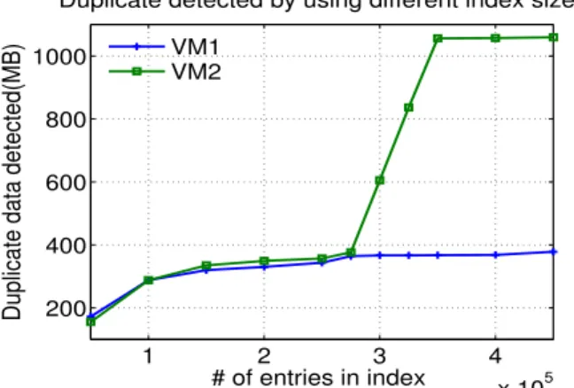
One intuitive alternative is to try and estimate the ap-propriate amount of memory that is needed prior to deploying the deduplication system. A straightforward approach is to perform simple profiling on a sample of data and compute the expected memory requirements based on the results. To illustrate why this is difficult to choose the right amount of RAM in practice, we conducted a simple experiment that represents a storage system used to archive virtual machine (VM) images (this is a common workload used in deduplication eval-uations [6], [12]). We want to maximize deduplication ratio to conserve bandwidth and storage costs. For sim-plicity, we assume that all VMs are running the same OS, and are the same size. A simple way to estimate memory requirements is to first estimate the index size for a single VM, and then use that to estimate the total RAM necessary for all users. Thus, given n users and each user stores the same size VM, we estimate m amounts of RAM to index one user such that our backup system will need n·m amounts of RAM. We can derive mvia experiments. Figure 2 shows the results for two VMs. As far as we know, VM2 contains more text files while VM1 has more video files. Number of index entry slots indicates how much information of already stored data the system can provide for duplicate detection. We set fixed number of index entries for duplicate detection and gradually increase it. We see that when index entry slots number increases to 270 thousand, both VMs exhibit the same amount of duplicate data. As we increase the index size, VM1 shows limited improvement, while VM2 shows much better performance. If we had used VM1 to estimatemwould have led to much less bandwidth sav-ings, especially if a significant number of VMs resemble VM2. Buying too much memory is wasteful if most of the data resemble VM1.
2.3.2 Using Locality And Downsampling
We hereby provide an overview of basic sampling ap-proached by [5], [6], followed by a discussion on the ad-vantages of sampling and its limitations. Storage systems that make use of data deduplication generally operate on chunk-level, and in order to quickly determine potential duplicate chunks, an index for existing chunks needs to be maintained in memory. For example, a 100TB data will need about 800GB RAM for the index under standard deduplication parameters [13], which makes keeping the entire index in memory challenging. Typical
1 2 3 4 x 10⁵ 200 400 600 800 1000 # of entries in index
Duplicate data detected(MB)
Duplicate detected by using different index sizes VM1
VM2
Fig. 2: Intuitive test on amount of duplicate detected on two equal-sized(4.7GB) VMs by using equal-size indexes
deduplication parameters which have been experimen-tally shown to give good performance [13] is given in Table 2. We see that in order to support 12.5 billion (100TB/8KB) chunks, we need 800GB amounts of RAM for the index. As data size increases to 300TB, we need to support all 37.5 billion chunks, and 2400 GB of RAM is needed only for indexing (C ∗E/ck = 2400∗ 109).
These estimated figures are naturally conservative, since the actual amount of replicated chunks are unknown at run time. The principle of locality is used to design sampling algorithms that utilize smaller index size while providing good performance [5]. The locality principle suggests that if chunk X is observed to be surrounded by chunks Y, Z, W in the past; the next time chunk X appears, there’s a high probability that chunks Y, Z, W will also appear. In sampling-based deduplication, the data will be first divided into larger segments, each of which contains thousands of chunks. Deduplication is executed based on these segments by identifying existence of their sampled chunks’ fingerprints in the index. If a chunk’s fingerprint is found in the index, the correspondent segment which contains that chunk will be located and fingerprints information of all the other chunks in this segment will be pre-fetched from disk to the chunk cache in memory. Downsampling algo-rithm [6] works as an optimized sampling approach, by taking advantage of the locality principle. The difference is that the sampling rate is initialized as 1, i.e., it picks all the chunks in a segment as its sampled chunks. As the amount of incoming data increases, this value gradually decreases by dropping half of index entries. Thus the indexing capacity doubles by only accepting a part of chunks’ fingerprints as samples to represent each segment. In other words, instead of indexing chunks X, Y, Z, and W in RAM, the downsampling algorithm will only index chunk X (or another one among four of them) in RAM after two times of adjustments, and the rest on disk. The above sampling-based approaches have two main drawbacks. The first (obvious) drawback is that not all data exhibit locality [14], and thus sampling algorithms do not work well with these datasets. The second drawback is that even for data that exhibits
Terminology Value
Chunk sizeck ck= 8KB
Segment sizeS S= 16M B Physical storage capacityC C= 300T B Number of chunksN N=C/S Index entry sizeE E= 64B
TABLE 2:An example of a cloud-base backup system configu-ration
locality, it is difficult to select the correct sampling rate or how to adjust it, due to the large variance in possible deduplication ratio [15] [16].
2.4 Understanding Elasticity Awareness And Scal-ing Up
Our last direction is to dynamically scale up the storage system during runtime. After several downsampling operations, the assigned RAM may still not large enough to process the incoming data stream. Then we need to trigger the online scaling up operation, which is taking advantage of cloud computing’s elasticity fea-ture. Scaling up operation can improve deduplication systems by allowing deduplication storage systems to dynamically adjust the amount of memory resources as needed to detect sufficient amount of duplicate data. This is especially useful when the index used for dedu-plication is often kept within the memory to avoid the performance bottleneck from disk I/O operations. There are two problems in elasticity awareness and scaling up operation:
1) When to trigger the scaling up operation? The main guide is to trigger the scaling up op-eration only when the result can benefit to the performance. We need to distinguish whether poor deduplication performance is due to overly ag-gressive downsampling (caused by user’s high ex-pected deduplcation degree) or inherent within the dataset type (dedup-unfriendly datasets that have low duplication ratio). To solve that, we need to answer these three questions: (i) if the the RAM (for the cached index) is close to the preset limitation, how does system detects and evicts some non-critial entries? (ii) when does the system need to trigger downsampling process? (iii) after how many times of downsampling, the system finally requests to scale up?
2) How to assign new resources?
Both the pricing costs and resource utilize ra-tios should be considered when assigning new resources. A straightforward strategy is to simply double (or preset n times) the current size when scaling up. However even regardless of the high expense, this exponential expansion brings a big waste since later incoming stream may not need so large space. An optimized approach is required to obtain higher RAM utilization efficiency, which should expend RAM size based on the occurrences of downsampling which may predict the dataset’s future.
3
EAD: E
LASTICITY-A
WARED
EDUPLICATION Storage deduplication services in the cloud often run in virtual machines (VM). Unlike a conventional OS which runs directly on physical hardware, the OS in a VM is running on top of a hypervisor or virtual machine moni-tor, which in turn, communicates with the underlying physical hardware. The hypervisor is responsible for increasing RAM resources to the virtual machine (VM) dynamically. This can be done in two generic ways.The first is to use a ballooning algorithm to reclaim memory from other VMs running on the same physical machine (PM) [17]. This is a relatively lightweight pro-cess that relies on the OS’s memory management algo-rithm, but can only increase relatively small amounts of memory. Deduplication systems that require increasingly larger amounts of memory need to run a VM migration algorithm [18], [19]. In VM migration, the hypervisor migrates the RAM contents from one PM to another with sufficient memory resources [18]. Regardless of the mi-gration algorithm used, some downtime can inevitably occur when switching over to a new VM [19].
The second is a naive approach towards incorporating elasticity is to increase the memory size once the index is close to being full. This naive approach does not perform well since frequent scaling up or migration induce a high overhead. Furthermore, the naive approach always retains the entire old index during each scaling up or migration, even those index entries do not finger print many chunks. Such poor performing index entries take up valuable index space without providing much benefits.
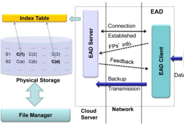
Our approach combines the benefits of downsampling [6] and VM scaling up to allow users to maintain a satis-factory level of performance by adjusting sampling rate and memory size accordingly. Our system design con-sists of two components, anEAD clientthat is responsible for file chunking, fingerprint computation and sampling, and anEAD serverwhich controls the index management and other memory management operations. The EAD clientis run on the client side, for instance, at the gateway server for a large company. The EAD server can be executed by the cloud provider. The entire system design is shown in Figure 3. Only unique data is supposed to be store in Physical Storage. The File Manager is responsible for data retrieval and maintenance, how it works is out of this paper’s scope.
3.1 EAD Algorithm
Different types of users have different deduplication requirements. Some users will be willing to tolerate worse deduplication performance in exchange for lower costs, while others will not. To accommodate different requirements, EAD is designed to allow a user to specify a scaling up (or migration) trigger, Γ (∈ (0,1)), which specifies the level of deduplication performance the user is willing to accept.
Fig. 3:EAD infrastructure.
Deduplication performance is usually measured by reduction ratio[20], [21], which is the size of the original dataset divided by the size of the dataset after dedupli-cation. To help the user select the migration trigger, we define Deduplication Ratio (DR),
Deduplication Ratio= 1−Size after deduplication
Size of original data (1) Intuitively, we would like to first apply downsampling algorithms until the deduplication performance becomes unsatisfactory, and then migrate the index to larger memory in order to obtain better performance. EAD will migrate to larger RAMonlywhen migration will result in deduplication performance better thanΓ. This has an important but subtle implication.EAD will not always migrate when deduplication performance falls under Γ, but only when migration will improve performance. This is important because given a dataset that inherently exhibits poor deduplication characteristics [22], adding more RAM will incur the migration overhead without improving deduplication performance. This means that EAD cannot simply compare the measured DR against Γ because the measured DR may not necessarily reflect the amount of duplication that exists. To illustrate, let us assume that the deduplication system measures its DR and it is less thanΓ. There are two possibilities. The first is that the system has performed overly aggressive downsampling, and can benefit from increasing RAM. The second possibility is that the dataset itself has poor deduplication performance, e.g. data in multimedia or encrypted files. In this case, increasing RAM does not result in better performance. How our EAD algorithm determines when to migrate to more RAM resources can be found in Alg. 2. It executes in two phases as generic in-line deduplication systems do. We use Sin and x to
denote the incoming segment and chunks inside it.F Px
represents the fingerprint of chunkx. InPhase ItheEAD Client sends all chunks’ fingerprints information (F Pxi)
(∀xi ∈ Sin) , including labeling F Pxiest and F Pxidedup of
sampled chunks used for estimation and duplication detection, in each segmentSin toEAD Server. The latter
will search index tableTandchunk cachefor duplication identification, as well as updatingestimation baseB. Each chunk xi is then marked as duporuniq, indicating it is
unique data chunks along with metadata of duplicate ones to EAD Server in Phase II, saving bandwidth and storage space. At the meantime, current sampling rate R0 is subject to change to R based on deduplication performance. Details on features of the EAD algorithm will be presented next.
3.2 Estimating Possible Deduplication Performance One of the key features of EAD is that the algorithm is able to determine whether migration will be benefi-cial. In order to distinguish whether poor deduplication performance is due to overly aggressive downsampling or inherent within the dataset, we first need to be able to estimate the potential DR of the dataset. Obtaining the actual DR is impractical since it requires performing the entire deduplication process. Prior work from [23] provided an estimation algorithm to estimate the dedu-plication performance for static, fixed-size data sets. Their algorithm requires the actual data to be available in order to perform random sampling and comparisons. However, in our problem, the dataset can be viewed as a stream of data. There is no prior knowledge of the size or characteristics of the data to be stored in advance. We also cannot perform back and forth scanning of the complete dataset for estimation. In our EAD algorithm, we let theEAD Servermaintain anestimation baseB. The EAD Client randomly selects κ fingerprints from each segment and sends them to EAD Server to be stored in B. Suppose there are ns segments come in, there will
be κ·ns samples, which will increase along with the
increasing amount of incoming data. Each entry slot in B includes a fingerprint as well as two counters, xc1 and xc2, where counter xc1 records the number of occurrences of fingerprint F Px appears in the B, and xc2 records the number of occurrences of fingerprint F Pxappears among that of all the chunks uploaded. We
integrate our estimation process into the regular dedu-plication operations so as to avoid the separate sampling and scanning phases by [23]. While the client sends the samples for duplication searching to the storage server, these samples for estimation are transmitted at the same time for updating B. During the fingerprint comparison of incoming chunks against that in chunk cache, we update B again, incrementing the counter xc2 by one every time its correspondent fingerprint appears. Thus, there is no extra overhead for our estimation purpose. Using B, we can compute the estimated deduplication ratio, EDR, as EDR= 1− 1 κ·ns X x∈B xc1 xc2 . (2)
The computation of EDR happens while the index size is approaching the memory limit. Only in the case that DR is smaller thanΓ·EDR, there will be a potential performance improvement by migration, and EAD will migrate the index to larger RAM. Otherwise, EAD will apply downsampling on the index as the exchange for larger indexing capacity.
Algorithm 2 Elastic deduplication strategy 1: The incoming segmentSin:
Deduplication Phase I: Identify duplicate chunks 2: ∀xi∈Sin: EAD Client sendsF Pxi to EAD Server
3: for allF Pdedup
xi do
4: ifF Pxidedup∈T then
5: Locate its correspondent segments Sdup ∀xj ∈Sdup: Fetch information ofxj (F Pxj)
Setxj∈chunk cache
6: else
7: AddF Pdedup xi toT
8: for allF Pest xi do 9: ifF Pest xi ∈B then 10: xic1 =xic1+ 1 11: else 12: AddF Pest xi toB Setxic1 =xic2 = 0 13: for allxi∈Sin do
14: ∀xk ∈chunk cache: CompareF Pxi with F Pxk
15: ifF Pxi =F Pxk then
16: Setxi∈dup(xdupi )
17: else
18: Setxi∈uniq (xuniqi )
19: ∀xl∈B:Compare F Pxi withF Pxl
20: ifF Pxi =F Pxl then
21: xic2 =xic2+ 1
Deduplication Phase II: Data transimission 22: for allxi∈Sin do
23: Transmits xuniqi along with only metadata ofxdupi 24: EAD finishes processing Sin
25: ifIndex is approaching the RAM limitthen 26: ifDR<Γ·EDRthen
27: ifR0= 1 then 28: EAD sets Γ = EDRDR 29: else
30: EAD triggers migration, setting rateR= ∆·R0 31: else
32: EAD sets R= R0
∆
3.3 EAD Scaling Up Algorithm
The performance of the EAD algorithm can be further improved by observing additional information obtained during the run time and then adjusting the parameters of the algorithm.
(1) Adjusting Γ. The parameterΓ is specified by the user, and indicates the user’s desired level of dedupli-cation performance. However, the user may sometimes be unaware of the underlying potential deduplication performance of the data, and set an excessively high Γ value, resulting in unnecessary migration over time. We adjust the user’s Γ value to DR
EDR after each migration,
and also in the case that DR has not reached accepted performance even the sampling rate is one. So that it represents the current system’s maximum deduplication ability. In this way, EAD is able to elastically adapt variations on incoming data.
(2) Amount of RAM Post Migration. A simple way to compute the amount of RAM is allocating after mi-gration by using a fixed sized∆, e.g. doubling the RAM each time (∆ = 2). We then reset the sampling rate back to 1, and start all over again. Another way is based on the observation that the sampling rate before the latest downsampling operation is able to support a satisfying performance, so that EAD will adjust current sampling rate to the one before latest downsampling operation. Thus, the specific amount of incoming data will require different amount of index spaces based on the adjusted sampling rate, implying that there exists subtle relations among R0, ∆ and size of RAM. When deduplication performance may be not satisfactory, EAD will migrate to more RAM as well as applying a higher sampling rate for future deduplication. A simple approach could be that RAM increases at the same changing rate (∆) of sampling rate. We can improve over this process by observing the next to last sampling rate used prior to migration. This rate is the last known sampling rate that produced acceptable deduplication performance. This is valid because if it didnotproduce an acceptable perfor-mance, EAD would have already triggered migration. We hereby propose to utilize a more conservative index RAM incrementation policy based on above analysis. We introduce a parameter d (initialized as zero) to record occurrences of downsampling, every time the downsam-pling happens,dincreases by one. We set the New Index Size (RAMnew) after migration following the rule:
RAMnew= ( ∆·RAMorg d= 1 ∆·[1−Pd−1 i=1 1 ∆i]·RAMorg d≥2 (3) Where RAMorg represents the original index size
be-fore migration. As the times of downsampling operation increase, EAD requires less amount of RAM for index table after migration. Compared with always requiring ∆ times of original RAM, such optimized approach is able to claim higher memory utilization efficiency.
(3) Managing Size ofB.One concern with our estima-tion scheme is that the size of Bmay become too large. If we need a large amount of RAM to storeB, we will be wasting RAM resources that could be used in the index. In practice, the size ofBis relatively modest. Each entry in B consists of a fingerprint and two counters. Using SHA-1 to compute the fingerprint results in a 20 byte fingerprint. An additional four bytes are used for each counter. Thus, each B entry is28 bytes, indicating that the total size ofBwould be at most approximately 33.38 MB to support 1 TB of data. In our experiment, it only requires 4.32 MB for estimating 163.2 GB dataset. 3.4 Scaling Up Strategy
While the scaling up (migration) has finished, we are left with the original index (copied over), and space for the new index, also the system will apply a new sampling rate, which is higher than original one, in order to keep a satisfying deduplication performance. At this stage, EAD
will compensate the poor deduplication performance due to previously too sparse sampling rate in two steps: 1) Search through the original index table, re-detect duplication chunks from already stored segments. Notice that the read/write operations may bring unexpected cost, so that EAD only process limited number of segments which are able to claim dupli-cate chunks. Detailed mechanism will be explained later.
2) We know that it is possible not all index entries in the old index are useful, meaning that some entries contain fingerprints for chunks that are unlikely to be encountered again. Keeping these entries in the new merged index will waste index slots. Therefore, after migration and duplication re-detection, these entries are removed from the index table.
To identify segments that contain undetected duplicate chunks is a nontrivial task. As a sampling approach, data segments are only represented by their sampled chunks, whose fingerprints are stored in the index. Thus EAD have to identify those segments only by searching through index table. We propose to inject additional information into index to assist finishing this task: a counter (countF P, initialized as zero for new added
entries) is used for each index entry to record its hitting times, which we call hitting rate. Every time when an entry has been found a match, this counter increments by 1. Therefore the larger the counter is, the more duplicate chunks this entry can detect. Among those segments hooked by FPs with low hitting rate, there exists ’evicted’ duplicate chunks. This conclusion is derived based on the following analysis of FPs in the index:
• Entries with high hitting rate. These FPs in the index indicates that segments have found matches and lots of chunks near the sampled chunks are identical, which is the natural results of chunk local-ity. Theoretically, the higher hitting rate they have and the more entries which have such high hitting rate, the more space will be saved.
• Entries with low hitting rate. The explanation for them: some segment themselves share few chunks with stored ones, resulting in lower index matching rate; other of them share lots of chunks with stored segments, however they are not hooked by right FPs because of sparse sampling rate, thus no or not enough matches are found from their sampled chunks’ fingerprints in index.
Majority of duplicate chunks evicted could be elim-inated from segments who are indexed by FPs with low hitting rate. Compared with reprocessing all the segments on the storage, EAD is able to select only part of them for detecting majority duplicate evictions based on their hitting rate: It uses entries with low hitting rate to track their correspondent segments and detect evicted duplicate chunks. The threshold for labeling hitting rate as high or low is not arbitrary. Suppose
that we have n chunks come in for a backup process, the measured Deduplication Ratio is fmr (fmr < Γ · EDR). At the meantime, we have counters’ values as
{0,1,· · · , c,· · · , m}, their correspondent amount of en-tries are{n0, n1,· · · , nc,· · ·nm} (i.e. There aren0 entries whose counter values are zero, etc.). Therefore the total ’eviction’ amount of chunks (nevt) which are expected to
be found duplicate on the cloud is calculated as: nevt=n·(Γ·EDR−fmr) (4)
Assume that the original sampling rate is R0, thus the minimum number of index entries to be selected is R0 · nevt. Based on above calculation, EAD starts
picking index entries with counter value as zero (n0), if n0 < R0·nevt, EAD picks entries with hitting rate as
one and vice versa. Until it satisfies:
c X
i=0
ni≥R0·nevt(0≤c≤m) (5)
By doing this, those segments that are mostly potential for improving deduplication performance are identified. Then we locate segments indexed by these FPs, choosing new set of samples as well as detecting duplicate chunks from them. We illustrate above process in details as Algorithm. 3. Choosing new set of samples will result extra FPs, which will be put into the additional RAM as a part of new index table. Besides, based on former analysis, those entries lead to poor performance are removed from original index table, which could claim additional savings on RAM, making our solution more memory efficient. Furthermore, to avoid adding them back to the index table, a Bloom Filter(BL) [24] is used on the cloud server to record hash information of removed FPs. By doing so, old index will not be entirely kept and valuable index space will be released for future use. While scaling up finishes, EAD will merge old and new indexes, calculating updated Deduplication Ratio. If Deduplication Ratio is still lower than Γ·EDR after duplication re-detection, EAD will reset the value of Γ, making Γ·EDRequals to the value of current Dedupli-cation Ratio. So that the requirement on dedupliDedupli-cation performance will not surpass the system ability.
3.5 Storage Hierarchy
The basic design is a classical simple two-level hierarchy: RAM for IndexTable (along with other metadata ta-bles like EstimateBaseand ContainerRecord) and ChunkCache, and MD for SegmentChunkHash. In de-tail, for the RAM level, we divide the RAM into several partitions (note that the RAM mentioned here only means the user accessible RAM part, which ignores the part occupied by the operating system as well as other background apps): the first partition is for caching IndexTable and some counters, which will keep oc-cupying more and more space in RAM during runtime. Therefore the larger of available RAM assigned for it is, the higher hit ratio the system can achieve. On the other
Algorithm 3 Elastic scaling up strategy
1: The index entry x (with fingerprint F Px) has been
chosen
2: Locate its correspondent segment Segx
3: ifSegx has not been processedthen
4: Select new sample chunks from Segx based on
current sampling rate
5: for new sampled chunk (with fingerprint F Py)
se-lected do
6: if F Py finds matching record in the new index
(F Py=F Pj,F PjF Pnewindex)then
7: LocateSegj and pull out its FPs to chunk cache
for duplication re-detection 8: else
9: F Py has been added into the new index as a
new entry slot
10: for α= 1 :total number of chunks inSegx do
11: Compare F Pα with those inSegj
12: ifF Pαfinds match then
13: Chunk αis duplicate
14: Entry x will be removed from old index, Bloom Filter records information of F Px
hand, the second RAM partition is an isolated temporary loading area, which storesChunkCache(meta data of all chunks from a certain segment), and data there will be not useful after the comparison process is finished. In an-other word,ChunkCachewill not keep occupying more and more space in RAM. For the MD level, the entire database of SegmentChunkHash is stored here. When there is a hit miss in the RAM, existing chunks’ metadata are loaded from MD to RAM, and new segments and chunks’ data are updated into MD. However, there are two main limitations of this design: (i) small RAM size results in frequently evicting cached IndexTable and lower the hit ratio; and (ii) MD’s low access speed will extremely decrease the overall speed. Thus, to improve the deduplication speed, we need to increase the cache hit in RAM’s IndexTable partition and speedup MD access.
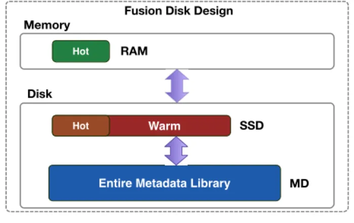
Before we design new hierarchy of RAM, SSD and MD, we need to consider these two question: (i) when does it make economic sense to make a piece of data resident in RAM? and (ii) when does it make sense to have it resident in disk? The answer is that RAM keeps most frequently used IndexTableso that the hot data can be accessed from a higher speed storage RAM. In another word, RAM (a higher speed storage level) is a typical cache of MD (a lower speed storage level). A feasible solution (as shown in Figure 4) is to use the SSD as the cache of the MD, which unifies a high-speed SSD and a large-capacity hard drive. We name it as the “Fusion Disk” (FD) design. Basically, this design focuses on improving the disk set’s overall access speed, so we do not need to change any behavior between RAM to the disk set in our deduplication system. RAM stores
9 HotData, while SSD stores bothHotData (as a copy of
RAM) and W armData.
Memory
Warm
Entire Metadata Library
Hot
RAM SSD
MD
Fusion Memory Design
Disk
Memory
Warm
Entire Metadata Library
Hot RAM
SSD
MD Fusion Disk Design
Disk
Hot
Fig. 4:Structure of fusion disk design
The last question is “what caching algorithm should be applied on the SSD?”. These following things are key concerns for caching algorithms: (i) when and what at to put in the cache or slow storage when facing with new incoming data; (ii) when and what to admin from the slow storage to cache; and (iii) when and what to evict from cache to slow storage. In the baseline EAD design, we use LRU algorithm which discards the least recently used items first. In general, there is no one single algorithm fix all traces. Thus, we need to conduct a trace-driven simulation test to analyze different algorithms.
4
E
VALUATIONIn our evaluations, we collected a dataset consisting of VMs that all run the Ubuntu OS, but each VM has differ-ent types of software and utilities installed and contains different types of application data, which majority comes from Wikimedia Archives [25] and OpenfMRI [26]. The total size of our dataset is around 163.2 GB. We eval-uate our solution, denoted as Elastic in the figures, against two alternatives approaches. The first alternative, denoted as FullIndex, represents an ideal situation where there is unlimited RAM available. This will serve as an upper bound on the total amount of space savings. The other alternative is denoted asDownSample, which is a recent approach [6] that dynamically adjusts the sampling rate to deal with insufficient RAM.
4.1 Deduplication Ratio
We hereby compare our algorithm with a generic dedu-plication mechanism without sampling and a state-of-art high performance deduplication strategy with down-sampling mechanism [6]. Before deploying the dedupli-cation process, we allocate a specific amount of RAM for index in different strategies. Table 3 shows the amount of RAM allocated for different deduplication strategies.
We set the size of each entry slot in the index as 64 bytes, which consists of three parts: FP, chunk metadata (storage address, chunk length,etc) and counter, which is 20 bytes (SHA-1 hash signature [27]), 40 bytes and 4 bytes, respectively. These sizes may vary under different
Strategy # of index entries size of index(MB)
Full index 10×106 640
With down-sample 5×10⁵ 32
EAD 1×10⁵ 6.4
TABLE 3: RAM deployment for index under different dedu-plication strategies. We set the down-sampling trigger as 0.85, which means while the storage is approaching85%of its cur-rent limit, the index will be down-sampled (Half of its entries will be removed. e.g., delete index FPs withF P mod2 = 0). hash functions or addressing policies, however it will not differ too much. We assume that the capacity is 75 GB. Nearly 10 million index entries are needed to index all the unique data if we do not use any sampling strategies. While under the down-sample strategy with the minimum sampling rate of 0.05, we need 500K index entries for 75 GB of unique data. EAD always picks a much more conservative size of index, specifically only 100K entry slots in this case.
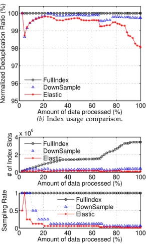
We here use Normalized Deduplication Ratio as the metric for deduplication ratio comparison. It is defined as the ratio of measured Deduplication Ratio to Dedu-plication Ratio of FullIndexdeduplication. Note that FullIndex detects all the duplicate data chunks and can claim highest deduplication ratio. Thus, such a metric is meaningful because it indicates how close the measured deduplication ratio is to the ideal deduplica-tion ratio achievable in the system. Figure 5a shows the Normalized Deduplication Ratio of the above deduplica-tion strategies. Downsampling and computadeduplica-tion ofEDR happen when the usage of index approaches 85% of its capacity. For the down-sample strategy, it has the ratio higher than 99.5 %, showing the benefits of taking ad-vantage of locality. The EAD does not claim equally high ratio, however the gap is less than 2 %. Also consider that the performance requirement for EAD is defined by Γ, which is 0.95 in this case, the performance ofElastic is always higher than 98%, performing better than what is required. Notice that the ratio shows us fluctuations, which indicates the inconsistency on data content among different VMs. When about 5% of data has been pro-cessed, there is a performance thriving, which cannot appear in DownSample. This can be explained that because of trivial size of initial index size, Elastic cannot detect enough duplicate chunks, leading to a poor performance, which triggers the migration and thrives its performance. Such elastic behavior is the unique feature which cannot be observed in the other two ap-proaches. However, purely comparing the deduplication ratio is not fair for evaluating their performance. Since that these three strategies spend different amount of RAM for index from the start. Figure 5b shows how sampling rate and number of index slots used vary above cases. Obviously, it brings too much memory cost without sampling. We notice that bothDownSampleand Elastic have comparatively very low memory cost (small number of index entry slots). Also we can observe that when about 5% of data has been processed, the sampling rate inElasticincreases, reflecting its feature
of elasticity. The above results show that EAD is able to use less RAM space to achieve a satisfying deduplication ratio, which is only slightly lower than the other two. Next we derive a more meaningful metricDeduplication Efficiency, as a single utility measure that encompasses both deduplication ratio and RAM cost, to make a more fair comparison among these three strategies.
(a)Deduplication ratio comparison.
0 20 40 60 80 100 95 96 97 98 99 100
Amount of data processed (%)
Normalized Deduplication Ratio (%)
FullIndex DownSample Elastic
(b)Index usage comparison.
0 20 40 60 80 100
0 2 4x 10
6
Amount of data processed (%)
# of Index Slots
0 20 40 60 80 100
0 0.5 1
Amount of data processed (%)
Sampling Rate FullIndex DownSample Elastic FullIndex DownSample Elastic
Fig. 5: The sampling rate is 1 for all of them at the start of back up. The index migration in EAD is triggered when the normalized deduplication ratio drops below 95 % (Γ=0.95), after that, sampling rate doubles(∆=2).
4.2 Deduplication Efficiency
As discussed in Section 4.1, neither deduplication ratio nor memory cost alone can fully represent the system performance. Therefore we define:
Dedup Efficiency= Duplicate Data Detected Index Entry Slots (6) as a more advanced performance evaluation criterion. By using this criterion, we make more fairly comparisons among EAD and the other two solutions, as shown in Figure 6. It shows that Elastic outperforms both DownsampleandFullIndexon efficiency. Notice that Elastic always yields a higher efficiency, almost 4 times of that from Downsample and 30 times of that fromFullIndex. This is because that its elastic feature enables it to utilize as little memory space as possible to detect enough duplicate data as required, avoiding memory waste as the other two do.
0 20 40 60 80 100 0 20 40 60 80 100
Amount of data processed (%)
Deduplication Efficiency (MB/Slot)
FullIndex DownSample Elastic
Fig. 6:Deduplication efficiency performance. 4.3 SSD-based Fusion Disk Evaluation
In this section, we first illustrate what is stored in RAM, SSD and MD, and then introduce a set of performance metrics used for evaluating a caching system. Following that, we investigate several caching algorithms, and analyze their impacts on our new EAD infrastructure through extensive simulations. Sensitivity analysis on different RAM and SSD sizes is also conducted.
4.3.1 Storage Partitions (1) What is stored in RAM?
The memory of each server stores two parts of cached data: IndexTable (along with other meta tables) and ChunkCache. Note that in practice, we only adjust the size of the IndexTable partition (refer as the RAM size), and ignore the SegmentChunkHash part since it is a tiny temporary loading area simply for comparison of cached and new-coming fingerprinters. Moreover, we do not count write operations of real chunk content (to the storage pool), but only focus on index table access (on the server’s disk). To simplify the problem, we fix the size of one chunk’s metadata to be 4 KB which is enough for encoding and assembling other necessary metadata in a real deduplication system. In other word, the basic unit of the I/O accesses is 4KB in this paper.
(2) What is stored in SSD and MD?
The server’s disk contains an entire metadata library which maps chunks’ fingerprints (including other meta-data) with their physical addresses in the storage pool. In our FD design, the SSD lays on top of MD (having an entire metadata library) and plays the role of cache under the write back caching policy. For example, pages from the RAM are evicted to the SSD, and when the SSD is full, a victim page is then evicted to the MD.
4.3.2 Performance Metrics
Recall that in our new EAD infrastructure, we adopt SSDs as a middle storage tier between RAM and disks. Different caching algorithms such as LRU(Least Recently Used Updating), CLOCK [28], ARC [29], and CAR [30] can be used to manage the data set cached in the new middle tier. To explore the performance of EAD under
these different caching algorithms, we introduce two important performance metrics: I/O hit ratio and I/O operation cost. We consider a combination of these two metrics as a criterion to investigate the impacts of these caching algorithms.
(1) I/O Hit Ratio:I/O hit ratio is defined as the fraction of I/O requests that are served by Flash. Although SSD’s access unit is also 4KB, an I/O request might still cross more than one page. Therefore, we regard an IO request as a “hit” only when all of its associated pages are cached in SSD. Higher I/O hit ratio means that more I/Os can be accessed from Flash directly which accelerates the overall I/O performance. Thus, one of our primary goals is to increase I/O hit ratio for improving SSD utilization. (2) I/O Operation Cost: I/O operation cost can be represented as I/O response time or I/O throughput (e.g., IOPS). In this paper, we use I/O response time to evaluate the cost, for using MD and FD, as shown in Equation 7, where CIOResp and CF lashU pdate represent
the IO access cost and the Flash contents updating cost, respectively. All N terms indicate the access numbers of SSD Read (NSSDr), SSD Write (NSSDw), MD Read
(NM Dr), and MD Write (NM Dw), while allT terms (e.g., TSSDr and TM Dr) show the corresponding average I/O
latency for each operation. CM D = CIOAccess
= NM Dr·TM Dr+NM Dw·TM Dw CF D = CIOAccess+CF lashU pdate
= NSSDr·TSSDr+NSSDw·TSSDw +NM Dr·TM Dr+NM Dw·TM Dw (7)
The main difference between the I/O cost calculation of MD and FD design is that the I/O cost of FD con-sists of two parts: I/O access cost and Flash contents updating cost. Table 4 (a) further presents the related I/O operations costs for MD and FD in four different scenarios, i.e., read hit, read miss, write hit, and write miss. Besides read miss, our FD design always redirects I/Os from slow MD to fast SSD, which significantly reduce the total I/O response times. Table 4 (b) shows Flash updating cost, which is only for the FD design. For example, when newly accessed pages are administrated but the SSD is full, extra time is needed to flush (or evict) the dirty page(s) to MD. We hereby consider such data movements between SSD and MD as Flash contents updating cost and include it in the overall I/O cost.
Table 4(c) further shows the actual average I/O re-sponse times (in microseconds) of various types of I/O operations at both SSD and MD devices. These results were measured from an Intel DC S3500 Series SSD with the capacity of 80GB and a Western Digital WD20EURS-63S48Y0MD with2T Band 5400 RPM. Note that the tested basic I/O size is specified as 4KB according to the spacial granularity.
TABLE 4:Costs Calculation Inside Fusion Disk (SSD and MD) (a) Operations for MD and FD I/O access costs
Case read hit Read miss Write hit Write miss MD MD read MD read MD write MD write FD SSD read MD read+ SSD write SSD write
SSD write
(b) Operations for inner FD Flash update cost Case Evict dirty page
Cost SSD read+MD write
(c) Measured average I/O response times (µs) of SSD and MD Latency TSSDr TSSDw TM Dr TM Dw
4KRandom 135 58 7671 3922
TABLE 5: I/O hit ratios (%) of different caching algorithms under 10k-index-entries RAM size case.
Hit ratio 500MB 1GB 2GB 3GB 4GB LRU 63.8540 64.0175 64.1430 64.8733 64.9455 CLOCK 63.8730 64.0243 64.1558 64.8405 64.9673 ARC 63.9253 64.0603 64.9264 65.3155 66.0120 CAR 63.9177 64.0692 64.9276 65.4293 66.0665 CART 64.0357 64.5996 65.3089 65.1504 66.4699
4.3.3 Evaluation On Different SSD Sizes
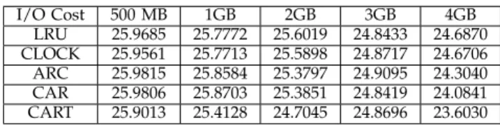
In this section, we evaluate the effectiveness of the FD design by conducting trace-driven simulations. The actual RAM size is fixed to 10k index entries, with deduplication chuck size as 8KB and segment size as 16MB, but the SSD size is varying from 500MB to 4GB. Different caching algorithms (e.g., LRU, CLOCK) are used to manage pages in SSDs. Table 5 shows I/O hit ratios under different SSD sizes when RAM is set to store at most 10k index entries. We first observe that all these algorithms achieve similar I/O hit ratios. Sophisticated algorithms like ARC, CAR and CART have slightly higher hit ratio than naive algorithms like LRU and CLOCK, because of their enhanced methods to avoid being flushed by I/O spikes. In general, the larger the SSD is, the higher hit ratio it will obtain. However as long as we has sufficient capacity to hold active working sets of all traces, the improvement in I/O hit ratio be-comes invisible. Similarly, Table 6 shows the normalized I/O operation costs under different SSD sizes (RAM’s upper bound is 10k index entries), where the cost under the MD design is used as the base line. We can see that our FD design is able to save almost 75% of I/O operation costs compared to the MD design. We interpret this benefit by observing that the FD design directs a large amount of I/Os to the SSDs which store hot data and thus reduces the I/Os to the MD, and consequently
TABLE 6:Total I/O response time costs normalized to no-SSD structure design (%) under 10k-index-entries RAM size case.
I/O Cost 500 MB 1GB 2GB 3GB 4GB LRU 25.9685 25.7772 25.6019 24.8433 24.6870 CLOCK 25.9561 25.7713 25.5898 24.8717 24.6706 ARC 25.9815 25.8584 25.3797 24.9095 24.3040 CAR 25.9806 25.8703 25.3851 24.8419 24.0841 CART 25.9013 25.4128 24.7045 24.8696 23.6030
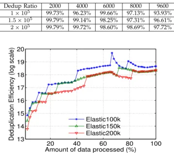
TABLE 7:The normalized deduplication ratios while we deploy different amount of memory for index (slots). The ratio is measured as every 200 incoming data segments have been processed,Γ = 0.9. Dedup Ratio 2000 4000 6000 8000 9600 1×10⁵ 99.73% 96.23% 99.66% 97.13% 93.93% 1.5×10⁵ 99.79% 99.14% 98.25% 97.31% 96.61% 2×10⁵ 99.79% 99.72% 98.60% 98.69% 97.72% 20 40 60 80 100 13 14 15 16 17 18 19 20
Amount of data processed (%)
Deduplication Efficiency (log scale)
Elastic100k Elastic150k Elastic200k
Fig. 7:EAD performance under different initial index sizes
saves the I/O operation costs. Moreover, we also observe that the larger the RAM is, the lower cost it can obtain. Similarly to I/O hit ratio, algorithms like ARC, CAR and CART save more time compared with LRU and CLOCK. 4.4 Scaling Up Evaluation
In this section, we evaluate the EAD strategy of the scaling up from different views. We first investigate the impact on initial index size (RAM size). We then focus on the memory usage comparison between our EAD and original down-sampling and full deduplication algorithms. We further conduct a scaling up experiment and adjusting both RAM and SSD size to see the corre-sponding I/O hit ratio and I/O response costs.
(1) Impact on initial index size.We first explore and verify the performance under different initial memory sizes for index. Table 7 shows the normalized dedupli-cation ratio as data comes in when initial index entry slots are 100K, 150K and 200K, respectively. It is not a surprise that a smaller index table helps to detect less duplicate data, but the gap is only at most approximately 4%. Another more interesting observation is that by applying our algorithm, initially smaller index table case
TABLE 8: The RAM cost is broken into index and estima-tion(Est.) parts for analyzing under different deduplication strategies. Γ = 0.95 and∆ = 2, respectively in this case. The unit of both initial index and final index size is slot. The unit of Est. and Total is MB.
Initial Index Final Index Est. Total
EAD 1×10⁵ 106581 4.32 10.82
Downsample 5×10⁵ 404818 0 25.91
Full Dedup 10×105 3441107 0 220.23
TABLE 9:I/O hit ratios comparison under different RAM and SSD size. We use number of cached index entries to represent the RAM size.
a a a a a aa SSD RAM 10k 30k 50k 70k 100k 500 MB 63.8540 86.9321 87.7542 92.2655 93.0350 1 GB 64.0175 87.0275 87.8919 92.3706 93.1250 2 GB 64.1430 87.1442 88.0682 92.4817 93.2558 3 GB 64.8733 87.4201 88.3375 92.6602 93.4129 4 GB 64.9455 87.4578 88.3985 92.6987 93.4612
TABLE 10:Total I/O operation costs comparison under differ-ent RAM and SSD size. We use number of cached index differ-entries to represent the RAM size.
a a a a a aa SSD RAM 10k 30k 50k 70k 100k 500 MB 25.9685 10.6303 10.2654 7.0243 6.5185 1 G 25.7772 10.5324 10.1390 6.9279 6.4398 2 G 25.6019 10.3923 9.9828 6.8341 6.3293 3 GB 24.8433 10.1052 9.7432 6.6778 6.1932 4 GB 24.6870 10.0372 9.6794 6.6449 6.1495
sometimes is able to claim even higher deduplication ratio. This is because it has a higher probability to be migrated so that there will be more index adjustments which brings performance improvement. Figure 7 shows the Deduplication Efficiency of EAD with different ini-tial memory sizes. It shows that the most conservative RAM initialization case claims the highest deduplication efficiency, which also proves that EAD provides well balance between memory and storage savings.
(2) Memory usage comparison. One of our goals is to introduce a comparable elasticity-aware deduplication solution to existing approaches. Based on above results, EAD is able to estimate (i) when to integrate new space for both RAM and SSDs for storing index table (including other necessary meta data), and (ii) what the integrated memory overhead and cost will be. We here compare it to state-of-art. Aside of memory space needed for index, EAD requires extra space for estimation. As shown in Table 8, the extra memory overhead of EAD mainly comes from the estimation part, compared with the other two. Even though, the total RAM cost by EAD is less than 50% and 5% of that by DownSample andFullIndex, respectively. Also note that there is 0.1 MB of index incrementation at the end of deduplication because of its conservative migration mechanism.
(3) Impacts of new SSD and RAM resources assign-ment.In our EAD design, when the performance benefit can be achieved, we trigger the scaling up operation assigning new RAM or SSD resources to store index tables. Here, we investigate the impacts of new RAM and SSDs assignment on I/O access performance. Table 9 shows I/O hit ratios under different amounts of RAM and SSDs during a real scaling up progress. The LRU algorithm is used here to manage the cached data. In general, increasing RAM and SSD size can dramatically improve I/O hit ratio. Moreover, we observe that the I/O hit ratio is more sensitive to the change of RAM
size than SSD. Table 10 further shows the corresponding I/O operation costs under different amount of RAM and SSDs. The cost under the MD design is used as the baseline. The larger RAM or SSD is assigned, the lower I/O operation cost is. Furthermore, adding RAM decreases I/O cost more efficiently than adding SSD.
5
RELATED
WORK
In this section, we review the related work in several cat-egories that are involved in this paper, namely, dedupli-cation, downsampling, and SSD and caching algorithms. (1) Deduplication:Numerous research has been done to improve the performance of finding duplicate data. Work by [31] focused techniques to speed up the dedu-plication process. Researchers have also proposed dif-ferent chunking algorithms to improve the accuracy of detecting duplicates [32]–[36]. Other research considers the problem of deduplication of multiple datatypes [14], [20]. This line of research is complimentary to our work, can be easily incorporated into our solution.
(2) Downsampling: The ever increasing amounts of data coupled with the performance gap between in-memory searching and disk lookups, mean that increas-ingly, disk I/O has become the performance bottleneck. Recent deduplication researches have focused on ad-dressing the problem of limited memory. Work by [4] proposed integrated solutions which can avoid disk I/Os on close to 99% of the index lookups. However, [4] still puts index data on the disk, instead of memory. Estimation algorithms like [37] can be used to improve the performance by reducing total number of chunks, but the fundamental problem remains as the amount of data increases. Other existing research in this area have proposed different sampling algorithms to index more data using less memory: [5] introduces a solution by only keeping part of chunks’ information in the index; and [6] proposes a more advanced method based on the work in [5] by deleting chunks’ fingerprints (FPs) from the index when it’s approaching fullness.
(3) SSD and caching algorithms: Many research works have been done to investigate the problem about how to best utilize the SSD resources as a cache-based secondary-level storage system or integrated with HDD as a hybrid storage system. Some conventional caching policies [38]–[41] such as LRU and its variants main-tain the most recent accessed data for future reuse while some other works intended to design a better cache replacement algorithm by considering frequency in addition to recency [42], [43]. [44] presented a SSD-based multi-tier solutions to perform dynamic extent placement using tiering and consolidation algorithms.
6
C
ONCLUSIONSAs a significant technique for eliminating duplicate data, deduplication largely reduces storage usage and bandwidth occupation in the enterprise backup systems.
Implementation of sampling further solves both chunk-lookup disk bottleneck problem and limited memory. In this paper, we first designed a multi-tier storage archi-tecture to improve caching capacity of current dedupli-cation systems. With such an enhanced system, we opti-mized deduplication approaches to achieve higher mem-ory utilization efficiency. However, when we adopted downsampling-based algorithms, we found that setting sampling rate only with the consideration of memory size cannot guarantee the performance of the whole system. We then proposed the elasticity-aware dedu-plication solution, in which dedudedu-plication performance and memory size are both considered. We detailedly showed EAD’s efficient adjustment on sampling rate by case analysis which shows that EAD claims much better performance than existing algorithms. Finally we proposed an online scaling up algorithm that takes advantage of the elasticity of cloud computing to dynam-ically trigger scaling up operation. Our algorithm offers a complete guideline for its large scale deployment. We conducted real trace driven simulations to evaluate the proposed approaches. The experimental result show that our design save at least 74% of overall I/O access cost compared to the traditional design.
REFERENCES
[1] D. Geer, “Reducing the storage burden via data deduplication,”
IEEE Transactions on Computer, 2008.
[2] T. T. Thwel and N. L. Thein, “An efficient indexing mechanism for data deduplication,” inCurrent Trends in Information Technology (CTIT), 2009.
[3] K. Srinivasan, T. d. Bissonet al., “iDedup: Latency-aware, inline data deduplication for primary storage,” inProceedings of the 10th USENIX conference on File and Storage Technologies, 2012. [4] B. Zhu, K. Li, and H. Patterson, “Avoiding the disk bottleneck in
the data domain deduplication file system,” inProceedings of the 6th USENIX Conference on File and Storage Technologies, 2008. [5] M. Lillibridge, K. Eshghi, D. Bhagwat, V. Deolalikar, G. Trezise,
and P. Camble, “Sparse indexing: large scale, inline deduplication using sampling and locality,” inProccedings of the 7th conference on File and storage technologies, 2009.
[6] F. Guo and P. Efstathopoulos, “Building a high performance dedu-plication system,” inProceedings of the 2011 USENIX conference on USENIX annual technical conference, 2011.
[7] A. Adya, B. diet al., “FARSITE: Federated, available, and reliable storage for an incompletely trusted environment,”ACM SIGOPS Operating Systems Review, 2002.
[8] G. Forman, K. Eshghi, and S. Chiocchetti, “Finding similar files in large document repositories,” inProceedings of the eleventh ACM SIGKDD international conference on Knowledge discovery in data mining, 2005.
[9] U. Manberet al., “Finding similar files in a large file system,” in
Proceedings of the USENIX winter 1994 technical conference, 1994. [10] B. Calder, J. d. Wanget al., “Windows Azure Storage: a highly
available cloud storage service with strong consistency,” in Pro-ceedings of the Twenty-Third ACM Symposium on Operating Systems Principles, 2011.
[11] “Amazon S3, Cloud Computing Storage for Files, Images, Videos,” Accessed in 03/2013, http://aws.amazon.com/s3/. [12] C. Kim, Park et al., “Rethinking deduplication in cloud: From
data profiling to blueprint,” inNetworked Computing and Advanced Information Management (NCM), 2011.
[13] G. Wallace, F. Douglis, H. Qian, P. Shilane, S. Smaldone, M. Cham-ness, and W. Hsu, “Characteristics of backup workloads in pro-duction systems,” in Proceedings of the Tenth USENIX Conference on File and Storage Technologies (FAST!’12), 2012.
[14] W. Xia, H. d. Jiang et al., “Silo: a similarity-locality based near-exact deduplication scheme with low ram overhead and high throughput,” inProceedings of USENIX annual technical conference, 2011.
[15] P. Kulkarni, F. Douglis, J. LaVoie, and J. M. Tracey, “Redundancy elimination within large collections of files,” inProceedings of the USENIX Annual Technical Conference, 2004.
[16] D. T. Meyer and W. J. Bolosky, “A study of practical deduplica-tion,”ACM Transactions on Storage (TOS), 2012.
[17] C. A. Waldspurger, “Memory resource management in VMware ESX server,”ACM SIGOPS Operating Systems Review, 2002. [18] F. Travostino, P. d. Daspitet al., “Seamless live migration of
vir-tual machines over the MAN/WAN,”Future Generation Computer Systems, 2006.
[19] C. Clark, K. Fraser, S. Hand, J. G. Hansen, E. Jul, C. Limpach, I. Pratt, and A. Warfield, “Live migration of virtual machines,” in
Proceedings of the 2nd conference on Symposium on Networked Systems Design & Implementation-Volume 2, 2005.
[20] D. Bhagwat, K. Eshghi, D. D. Long, and M. Lillibridge, “Ex-treme binning: Scalable, parallel deduplication for chunk-based file backup,” inModeling, Analysis & Simulation of Computer and Telecommunication Systems, 2009.
[21] M. Dutch, “Understanding data deduplication ratios,” inSNIA Data Management Forum, 2008.
[22] M. Hibler, L. d. Stoller et al., “Fast, Scalable Disk Imaging with Frisbee,” in USENIX Annual Technical Conference, General Track, 2003.
[23] D. Harnik, O. Margalit, D. Naor, D. Sotnikov, and G. Vernik, “Estimation of deduplication ratios in large data sets,” inMass Storage Systems and Technologies (MSST), 2012 IEEE 28th Symposium on, 2012.
[24] B. H. Bloom, “Space/time trade-offs in hash coding with allow-able errors,”Communications of the ACM, 1970.
[25] “Wikimedia Downloads Historical Archives,” Accessed in 04/2013, http://dumps.wikimedia.org/archive/.
[26] “OpenfMRI Datasets,” Accessed in 05/2013, https://openfmri. org/data-sets.
[27] J. H. Burrows, “Secure hash standard,” DTIC Document, Tech. Rep., 1995.
[28] L. A. Belady, “A study of replacement algorithms for a virtual-storage computer,”IBM Systems journal, vol. 5, no. 2, pp. 78–101, 1966.
[29] N. Megiddo and D. S. Modha, “Arc: A self-tuning, low overhead replacement cache.” inFAST, vol. 3, 2003, pp. 115–130.
[30] S. Bansal and D. S. Modha, “Car: Clock with adaptive replace-ment.” inFAST, vol. 4, 2004, pp. 187–200.
[31] A. Sabaa, P. d. Kumar et al., “Inline Wire Speed Deduplication System,” 2010, US Patent App. 12/797,032.
[32] L. L. You and C. Karamanolis, “Evaluation of efficient archival storage techniques,” in Proceedings of the 21st IEEE/12th NASA Goddard Conference on Mass Storage Systems and Technologies, 2004. [33] E. Kruus, C. Ungureanu, and C. Dubnicki, “Bimodal content defined chunking for backup streams,” inProceedings of the 8th USENIX conference on File and storage technologies, 2010.
[34] J. Min, D. Yoon, and Y. Won, “Efficient deduplication techniques for modern backup operation,”IEEE Transactions on Computers, 2011.
[35] A. Muthitacharoen, B. Chen, and D. Mazieres, “A low-bandwidth network file system,” inACM SIGOPS Operating Systems Review, 2001.
[36] K. Eshghi and H. K. Tang, “A framework for analyzing and improving content-based chunking algorithms,”Hewlett-Packard Labs Technical Report TR, 2005.
[37] G. Lu, Y. Jin, and D. H. Du, “Frequency based chunking for data de-duplication,” inModeling, Analysis & Simulation of Computer and Telecommunication Systems (MASCOTS), 2010.
[38] E. O’Neil, P. O’Neil, and G. Weikum, “The lru-k page replacement algorithm for database disk buffering,” inProceedings of the 1993 ACM SIGMOD international conference on Management of data, Washington, DC, 1993, pp. 297–306.
[39] M. Kampe, P. Stenstrom, and M. Dubois, “Self-correcting lru replacement policies,” inProceedings of the 1st conference on Com-puting frontiers, Ischia, Italy, 2004, pp. 181–191.
[40] T. Johnson and D. Shasha, “2q: A low overhead high performance buffer management replacement algorithm,” in Proceedings of the 20th International Conference on Very Large Data Bases, San Francisco, CA, 1994, pp. 439–450.
[41] Y. Zhou, J. Philbin, and K. Li, “The multi-queue replacement algorithm for second level buffer caches,” in Proceedings of the 2001 USENIX Annual Technical Conference, Boston, MA, 2001, pp. 91–104.
[42] N. Megiddo and D. Modha, “Arc: A self-tuning, low overhead replacement cache,” inProceedings of the 2nd USENIX Conference on File and Storage Technologies, San Francisco, CA, 2003, pp. 115– 130.
[43] D. Lee, J. Choi, J.-H. Kim, S. Noh, S. L. Min, Y. Cho, and C. S. Kim, “Lrfu: A spectrum of policies that subsumes the least recently used and least frequently used policies,” IEEE Transactions on Computers, vol. 50, no. 12, pp. 1352–1361, 2001.
[44] J. Guerra, H. Pucha, J. Glider, W. Belluomini, and R. Rangaswami, “Cost effective storage using extent based dynamic tiering,” in
Proceedings of the 9th USENIX Conference on File and Storage Tech-nologies, San Jose, CA, 2011.
Yufeng Wang is a 3rd year PhD student at Temple University under the supervision of Dr. Chiu C. Tan. He graduated from University of Electronic Science and Technology of China in 2012, majoring in Communication Engineering. His current research mainly focuses on efficient and secure data processing in cloud computing, mobile cloud computing, elastic memory man-agement and security enhancement.
Zhengyu Yangis a PhD candidate at the North-eastern University (since 2011 fall), under the supervision of Prof Ningfang Mi in NUCSRL lab. He graduated from the Hong Kong University of Science and Technology with a Master Degree in Telecommunication in 2011, and he obtained his Bachelor of Science Degree in Communication Engineering from Tongji University (Shanghai, China). His current research area is mainly on caching algorithm, cloud computing, deduplica-tion, and performance simulations.
Ningfang Mi joined Department of Electrical and Computer Engineering at Northeastern Uni-versity as an Assistant Professor in Fall 2009. Her research fields are capacity planning, re-source management, energy/power manage-ment, performance evaluation, system model-ing, simulation, virtualization, and cloud comput-ing.
Chiu C Tanis an assistant professor in the De-partment of Computer and Information Sciences at Temple University. He is a member of the Center of Network Computing. He is also the di-rector of the Temple University CIS Department REU program. His research interests lies in next generation computing systems, mobile and em-bedded sensor devices, high bandwidth wireless coverage, and cloud computing infrastructure.