Constraint Logic Program Execution
Manuel Carro
[email protected]
Manuel Hermenegildo
[email protected]
Abstract
Visualization of program executions has been found useful in applications which include education and debugging. However, traditional visualization techniques often fall short of expectations or are altogether inadequate for new programming paradigms, such as Constraint Logic Programming (CLP), whose declarative and operational semantics differ in some crucial ways from those of other paradigms. In particular, traditional ideas regarding flow control and the behavior of data often cannot be lifted in a straightforward way to (C)LP from other families of programming languages. In this paper we discuss techniques for visualizing program execution and data evolution in CLP. We briefly review some previously proposed visualization paradigms, and also propose a number of (to our knowledge) novel ones. The graphical representations have been chosen based on the perceived needs of a programmer trying to analyze the behavior and characteristics of an execution. In particular, we concentrate on the representation of the program execution behavior (control), the runtime values of the variables, and the runtime constraints. Given our interest in visualizing large executions, we also pay attention to abstraction techniques, i.e., techniques which are intended to help in reducing the complexity of the visual information.
Keywords: Execution visualization, Constraint Logic Programming, Constraint Programming.
1
Introduction
Program visualization has classically focused on the representation of program flow (using flowcharts and block diagrams, for example) or on the data manipulated by the program and its evolution as the program is executed (see, e.g., [BDM97, Mic97] for some recent examples). In this paper we address issues related to the visualization of the execution of Constraint Logic Programming (CLP) [JM94].1
Visualization of CLP executions is receiving much attention recently, since it appears that classical visualizations are often too dependent on the programming paradigms they were devised for and do not adapt well to the nature of the computations performed by CLP programs. Also, the needs of CLP programmers are quite different [Fab97]. Basic applications of visualization in the context of CLP, as well as Logic Programming (LP), include:
• Debugging. In this case it is often crucial that the programmer obtain a clear view of the program
state (including, if possible, the program point) from the picture displayed. In this application visualization is clearly complementary to other methods such as assertions [AM94, DNTM89, BDD+97] or text-based debugging [Byr80, Duc92, Fer94]). In fact, many proposed visualizations
designed for debugging purposes can be seen as a graphical front-end to text-based debuggers [DN94].
This work has been partially supported by ESPRIT LTR project DISCIPL # 22532 and CICYT Projects E96-1015-265 and TIC96-1012-C02-01. We wish to thank Kim Marriott, Peter Stuckey, Abder Aggoun, Helmut Simonis, Pascal Bouvier, Claude Lai, Christophe Aillaud and Pierre Deransart for discussions regarding this paper and constraint program visualization in general.
1Note that we are not concerned withvisual programming, although undoubtedly many ideas can be borrowed
or adopted from that paradigm.
• Tuning and optimizing programs and programming systems (which may be termed—and we will refer to it with this name—asperformance debugging). This is an application where visualization can have a major impact, possibly in combination with other well-established methods as, for example, profiling statistics.
• Teaching and education. Some applications to this end have already been developed and tested, using different approaches (see, for example, [EB88, Kah96]).
In all of the above situations, a good pictorial representation (either of the program data or of the program execution, depending on the objective) is key for achieving a useful visualization. Thus, it is important to devise representations that are well suited to the characteristics of CLP data and control. In addition, a recurring problem in the graphical representations of even medium-sized executions is the huge amount of information that is usually available to represent. To cope successfully with these undoubtedly relevant cases,abstractions of the representations are also needed. Ideally, such abstractions should show the most interesting characteristics (according to the particular objectives of the visualization process, which may be different in each case), without cluttering the display with unneeded details.
In this paper we explore, in the context of CLP, the topics mentioned above: the displaying of the execution and the data, as well as abstractions of those depictions. We propose designs addressing those topics, as well as implementations instrumenting those designs.
The aim of the visualization paradigms we discuss is quite broad—i.e., we are not committing ex-clusively to teaching, or to debugging—, but our focus is debugging, for correctness and, mainly, for performance. We divide the visualization paradigms into three categories (which, as we will see, can coexist together seamlessly, and even be used together to achieve a better visualization): visualizing the execution flow / control of the program, visualizing the actual variables (i.e., representing their runtime values), and visualizing constraints among variables. The three views are amenable to abstraction.
2
Visualizing Control
One of the main characteristics of declarative programming is the absence of explicit control. Although this theoretical property results in many advantages regarding, for example, program analysis and trans-formation, in practice programs are executed with fixed evaluation rules.2 Also, different correct
pro-grams can show wide differences in efficiency, and this efficiency often depends on the evaluation order. Understanding those evaluation rules is often important in order to write efficient programs (including termination, which obviously affects correctness). In this context, a good visualization of the program execution (probably combined with other tools) can help uncover performance (or even correctness) bugs which might otherwise be very difficult to locate.
In CLP programs (especially in those using Finite Domains) there are essentially two execution phases: the programmed search which results from the actual program steps encoded in the program clauses and the solver operations, which are the propagation steps performed inside the solver or in (generally, built-in) enumeration predicates.
2.1
Visualizing Control: the Programmed Search
The programmed search part of CLP execution is similar in many ways to that of LP execution. The visualization of this part of (C)LP program execution traditionally takes the form of a direct represen-tation of the search tree, whose nodes representcalls,successes,redos andfailures—i.e., the events which take place during execution. Classical LP visualization tools, of which the Transparent Prolog Machine (TPM [EB88]) is paradigmatic, are based on this representation. In particular, the TPM uses an augmented AND-OR tree (AORTA), in which AND and OR branches are somewhat compressed and take up less vertical space, but the information conveyed by it is basically the same as in a normal AND-OR tree.
It is true that in many CLP programs (and especially in those using Finite Domains) the control part has less importance than in LP, since the bulk of the time in such programs is spent in equation solving
2By “fixed” we mean that they can be deterministically known at every point in time, although maybe not
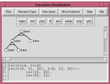
Figure 1: A small execution tree, as shown by APT
and enumeration. However, note that one of the main differences between C(L)P and, e.g., Operations Research is the ability to set up equations in an algorithmic fashion, and to perform search for the right set of equations, and thus it is still important during performance debugging to be able to represent and understand the control flow.
Thus, a first approach which can be used in order to visualize CLP execution is to represent the part corresponding to the execution of the program clauses (the programmed search) using a search-tree depiction. Note that the other important operations of CLP execution (enumeration/propagation) typically occur in “bursts” which can be associated to points of the search tree. Thus, the search tree depiction can be seen as a skeleton onto which other views of the state of the constraint store during enumeration and propagation (and which we will address in Section 2.3) can be grafted or to which they can be related.
In order to test this approach we have extended (in collaboration with INRIA) the APT tool (A Prolog Tracer[Lue97]) to serve as a CLP control visualizer. APT is essentially a TPM-based search tree visualizer, thus inheriting many characteristics from the TPM, but also adding some new, interesting features. APT is built around a meta-interpreter coded in Prolog which rewrites the source program and executes it, gathering information about the goals executed and the state of the store at runtime. This execution can be performed depth-first or breadth-first, and can then be replayed at will, and all the collected information can be displayed while re-executing. All the TPM windows are animated, and are updated as the execution of the program is replayed. The graphical part currently uses a Tcl/Tk interface, and runs under several systems (currently, SICStus [Swe95], and the clp(fd)/Calypso system developed at INRIA [DC93]).
The main visualization window of APT offers a tree-like depiction (Figure 1), in which the state of each node (not yet called, called but not yet exited, exited, failed) is shown by means of a color code. Nodes are represented by small squares and adorned optionally with the name of the predicate being called.
Clicking on a node opens a different window in which the relevant part of the program source, i.e., the calling body atom and the matching clause head, is represented, together with the (run-time) state of the intervening variables at that node. Note that only the presentation of these node views is dependent on the type of data (e.g., the constraint domain) used. This is one of the most useful general concepts underlying the design of APT: the graphical display of control is separated from that of data. This allows developing data visualizations independently from the control visualization, and using them together. The data visualization can then be taken care of by a variety of tools, depending on the data to be visualized. Following the proposal outlined above, this allows using APT without any change as a control skeleton for visualizing CLP execution. In this case, the windows which are opened when clicking on the nodes in the tree offer views of the constraint store in the state represented by the selected node. These views vary depending on the constraint domain used, or even for the same domain, depending on the data visualization paradigm used.
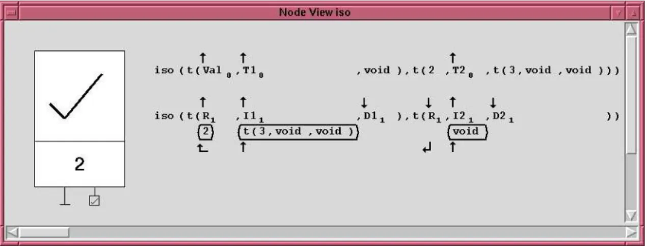
We will discuss several visualizations for constrains and constrained data in Sections 3 and 4. As an example of such a visualization, Figure 2 shows one depiction used for the Herbrand domain. The node
Figure 2: Detailed view of a node (Herbrand domain)
blow-up shows the run-time call on top and the matching head (below). The answer substitution (i.e., the result of head unification and/or body execution) is shown enclosed by rounded rectangles. The arrows represent the source and target of the substitution, i.e., the data flow.
As mentioned before, these node state windows are animated and evolve with the execution. Also, clicking on a substitution causes a line to be drawn in the main tree from the current node to the node where the substitutioncreated: this is a very powerful feature which helps in correctness debugging, as the probable source of a (presumably) wrong instantiation (causing, for example an unexpected failure or a bad value) can be easily located.
2.2
Time-based Depiction of Control
In our experience, tree-based representations such as those of the TPM, APT, and similar tools discussed above are certainly quite useful in education and, in part, for correctness debugging, i.e., finding logical errors. They are also useful to some extent in performance debugging, which aims at discovering the sources of unexpected low performance in a program. In some cases, the shape of the search tree can help in tracking down those sources, showing, for example, which computation patterns have been executed more often, or which parts dominate execution time, assuming similar time for every node. However, the lack of a representation of time (or, in general, resource consumption) information greatly hinders the use of simple search-tree representations in performance debugging. One approach in order to remedy this is to incorporate time (or other resource) information into the depiction itself, for example by making the distance between a node and its children reflect the elapsed time (or amount consumed of other resources). Such a representation intime spacenaturally provides insight into the cost of (different parts of) the execution. In such a CLP not all user-perceived steps (i.e.,callset al.) would show the same height: constraint addition, removing, unification, untrailing, etc. can have different associated costs in every program.
Time-oriented views have been used in several other (C)LP visualization tools, such as VisAndOr [CGH93] (included with recent distributions of SICStus [Swe95]) and VISTA [Tic92]. VisAndOr is a graphical tool aimed at displaying and understanding the performance of parallel execution of logic programs, while VISTA focuses on concurrent logic programs. In VisAndOr graphical depictions, time runs from top to bottom, and parallel tasks are drawn as vertical lines. These lines represent, using color and different thickness, which processor executes each task and the state of the task: running, waiting to be executed, or finished. In this case, the length of the vertical lines reflects accurately a measure of the time spent by the task. VisAndOr allows also switching to an events space, in which every event in the execution (say, the creation, the start, and the end of a task, among others), takes the same amount of space. Note that in this view the structure of the execution is easier to see, but the notion of time is lost—or, better, traded off for an alternate view. This events-oriented visualization is the one usually portrayed in the tree-like representation for the execution of logic programs: events are associated to the calls made in the program, and space is evenly divided among events. Thus events- and time-based visualization are not exclusive, but rather complementary to each other. VISTA representations are similar to those of VisAndOr, but time advances in a spiral.
2.3
Representing the Enumeration Process
The enumeration process typically performed by finite domain solvers (involving, e.g., domain splitting, choosing paths for constraint propagation, heuristics for enumeration) often critically affects performance. Observing the behavior of this process in a given problem (or class of problems) can often help understand the source of performance problems and flag that a different set of constraints (e.g., different constraints which model the same problem, or setting up more –or less– redundant constraints) or that a different enumeration strategy is needed.
The enumeration process typically takes the form of a search in whose branches the values of some variables are set and, as a result of the propagation of these changes, the domains of other variables also change. Each one of these steps results in either failure (upon which another path of the search is chosen by setting the chosen variable to another value or choosing another variable to set) or a new state with updated variable values. Thus, one approach in order to depict this process is to use the same depiction proposed for the programmed search, i.e., use a tree representation, in either time or events space. An alternative is to simply visualize those steps as a succession of states for all the variables (see Section 3.1 and, e.g., figures 5-6).
In some CLP systems, the enumeration and propagation parts of the execution are performed by internal built-ins. This complicates their visualization, since then, in order to gather data for the visualization, either the system itself has to be instrumented to produce the data (as in the CHIP visualizer [AS97]), or the sufficient knowledge about the solver operation must be made available so that its operation can be mimicked externally in a meta-interpreter inside the visualizer between actual execution steps.
2.4
Coupling Control Visualization with Verification
One of the techniques used frequently for program verification and correctness debugging is to use as-sertions which (partially) describe the specification and check the program against these asas-sertions (see, e.g., [AM94, DNTM89, BDD+97] and their references). Sometimes such assertions can be checked
stat-ically. When this is not possible, they can be incorporated in the program as run-time tests. Typically, a warning is then issued if any of these run-time tests fail, flagging an error in the program, since it has reached a state which does not meet the specification. It appears useful to couple this kind of run-time testing with control visualizations. Nodes which correspond to run-time tests can be represented in a special way, and color coded to reflect whether they succeed of fail. This allows to easily pinpoint the state of execution that results in the violation of an assertion (and, thus, of the specification) and, by clicking on the nodes above and to the left of the failed test, to explore for the sources of the error.
3
Displaying Variables
Typically, in imperative and functional programming there is a clear notion of the values that variables are bound to (although it is indeed more complex in the case of higher-order functional variables). The notion of variable binding in LP is somewhat more complex, due to the variable sharing which may occur among Herbrand terms. The problem is even more complex in the case of CLP, where such sharing is generalized to the form of implicit equations relating variables. As a result, the value of C(L)P variables often is actually a complex object representing the fact that each variable can take a (potentially infinite) set of values, and that there are constraints attached to such variables which relate them and which restrict the values they can take simultaneously.
Textual representations of the variables in the store are usually not very informative and not easy to interpret and understand.3 A graphical depiction of the values of the variables can offer a view
of computation states that is easier to grasp. Also, if we wish to follow the history of the program (which is another way of understanding the program behavior, but focusing on the data evolution), it is desirable that the graphical representation be either animated (i.e., time in the program is depicted in the visualization also in time) or laid out spatially as a succession of pictures. The latter allows comparing different behaviors easily, trading time for space.
3Also note that some solvers maintain, for efficiency reasons, only an approximation of the values the variables
1 2 3 4 5 6 X
Figure 3: Finite Domain depiction Figure 4: Shades representing age of discarded values Since different constraint domains have different properties and characteristics, different representa-tions for variables may be needed for them. In what follows we will sketch some ideas dealing with the representation of variables in commonly used constraint domains.
3.1
Depicting Finite Domain Variables
Finite Domains (FD) are one of the most popular constraint domains. FD variables take values over finite sets of integers which are the domains of such variables. The operations allowed among FD variables are pointwise extensions of common integer arithmetic operations, and the allowed constraints are the pointwise variants of arithmetic constraints. At any state in the execution, each FD variable has an active domain (the set of allowed values for that domain) which is usually accessible by using language primitives. For efficiency reasons, in practical systems this domain is usually an upper approximation of the actual set of values that the variable can theoretically take. We will return to this characteristic later, and we will see how taking it into account is necessary in order to obtain correct depictions of variable values.
A possible graphical representation for the state of FD variables (see [Mei96]) is to assign a dot (c.f., a square) to every possible value the variable can take; therefore the whole domain is a line (c.f., a rectangle). Values belonging to the current domain at every moment are highlighted. An example of the representation of a variable (X) with current domain {1,2,4,5} from an initial domain [1..6] is shown in Figure 3. More possibilities include using different colors / shades / textures to represent more information about the values (this is done also, for example, in the GRACE visualizer [Mei96]).
Looking at the static values of variables at only one point in the execution (for example, the final state) obviously does not provide much information on how the execution has actually progressed. However, the idea is that one such representation is associated with each of the nodes of the control tree, as suggested in Section 2, i.e., the window that is opened upon clicking on a node in the search tree contains a graphical visualization for each of the variables that are relevant to the node. The variables involved can be represented in principle simply side to side as in Figure 8 (we will discuss how to represent the relations between variables, i.e., constraints, in Section 4).
Note that, as mentioned before, often each node of the search tree represents several internal steps in the solver. The visualization associated to a node can thus represent either the final state of the solver operations that correspond to that search tree node, or the history of the involved variables variables through all the internal solver (or enumeration) steps corresponding to that node.
Also, in some cases, it may be useful to follow the evolution of a set of program variables throughout the program execution, independently of what node in the search tree they correspond to (this is done, for example, in the new visualizer for CHIP [AS97]). This also requires a depiction of the values of a set of variables over time, and the same solutions used for the previous case can be used.
Thus, it is interesting to have some way of depicting the evolution in time of the values of several variables. A number of approaches can be used to achieve this:
• An animated display which follows the update of the (selected) variables step by step as it happens; i.e., time is represented as time. This makes the immediate comparison of two different stages of the execution difficult, since it requires repeatedly going back and forth in time. However, the advantage is that the representation is compact and can be useful for understanding how the domains of the variables are narrowed. We will return to this approach later.
• Different shadings (or hues of color) can be used in the boxes corresponding to the values, repre-senting in some way how long ago that value has been removed from the domain of the variable (see Figure 4, where darker squares represent values removed longer ago). Unfortunately, com-paring shades accurately is not easy for the human eye, although it may give a rough and very compact indication of the changes in the history of the variable.
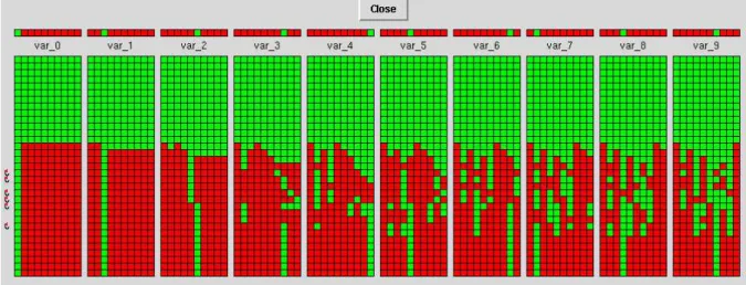
Figure 6: Evolution of FD variables for a 10 queens problem
• A third solution is to simply stack the different state representations, as in Figure 5, thus trading time for space. This depiction can be easily shrunk if needed to accommodate the whole variable history in a given space. It can reflect time accurately (for example, by reflecting it in the height between changes) or ignore it, working then in events space, by simply stacking a new line of a constant height every time a variable domain changes, or every time a enumeration step is performed. This representation allows easier easy comparison between states and has the additional advantage of allowing more time-related information to be added to the display. An example of the last approach above is one of the
visu-Figure 5: History of a variable alizations available in the VIFID visualizer, which we have
implemented at UPM, and which, given a set of variables in an FD program, generates windows displaying states or sets of states for those variables. VIFID can be used as a visu-alizer of the state in nodes of the search tree, or standalone, as a user library, in which case the display is triggered by spypoints introduced by the user in the program. Figure 6 shows a screen dump of a window generated by VIFID pre-senting the evolution of selected program variables in a
pro-gram to solve the queens problem for a board of size 10. Each column in the display corresponds to one such program variable. In this case the possible values are the row numbers in which a queen could be placed. Lighter squares represent values still in the domain, and darker squares represent discarded values. In this case, each row in the display corresponds to a spypoint in the source program, at which point VIFID consults the store and updates it. Points where backtracking took place are marked with small curved arrows pointing upwards. It is quite easy to see that very little backtracking was necessary, and that variables are highly constrained, so that enumeration (proceeding left to right) quite quickly discarded initial values. VIFID supports several other visualizations, some of which will be presented later in the discussion.
Some of the problems which appear in a display of this kind are the possibly large number of variables to be represented and size of the domains of each variable. Note that the first problem is under control to some extent in the approach proposed: if the visualization is simply triggered from a node in the search tree, the display can be selectively made to present only the relevant variables (e.g., the ones in the clause corresponding to that node). In the case of triggering the visualization through spy points in the user program, the number of variables is under user control, since they are selected explicitly when introducing the spypoints. The size of the domains of variables is more difficult to control (we return to this issue in Section 7). However, note that, without loss of generality, programs using FD variables can be assumed to initialize the variables to an integer range which includes all the possible values in the problem allowable in the state corresponding to the beginning of the program.4 Being able to deduce
a small initial domain for a variable allows starting from a more compact initial representation for that
1 2 3 4 5 6 X
Y Z
Figure 8: Several variables side to side
1 2 3 4 5 6 X
Y Z
Figure 9: Changing a domain variable. This in turn will allow a more compact depiction of the narrowing of the range of the variable, and of how values are discarded as the execution proceeds.
3.2
Herbrand Terms
Herbrand terms can always be written
X = f(Y,Z), X f Y Z
Y = a, X f a Z
W = Z, X f a Z W
W = g(K), X f a Z W g K
X = f(a,g(b)). X f a Z W g b
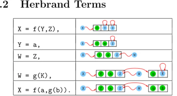
Figure 7: Alternative depiction of the creation of a Her-brand term
textually, or with a slightly enhanced textual representation, as in Figure 2. They can also be represented graphically, typically as trees. A term whose main functor is of arity n is then represented as a tree in which the root is the name of this functor, and the n sub-trees are the sub-trees corresponding to its ar-guments. This representation is well suited for ground terms. However, free variables, which may be shared by different terms, need to be represented in a special way. A possi-bility is to represent this sharing as just another edge (thus transforming the tree into an acyclic graph), and even, taking an approach closer to usual implementation designs, having a free variable to point to itself. This corresponds to a view of Herbrand terms as complex data structures with single assignment pointers. Figure 7 shows a representation using this view of the step by step creation of a complex Herbrand term by a succession of Herbrand constraints. Rational trees (as those supported by Prolog II, III, IV) can also be represented in a similar way—but in this case the graph can contain cycles, although it cannot be a general graph.
3.3
Intervals
In a broad sense, intervals resemble finite domains: the constraints and operations allowed in them are analogous (pointwise extensions of arithmetic operations), but the (theoretical) set of values allowed is continuous, which means that an infinite set of values are possible, even within a finite range. Despite the differences, similar visual representations to those proposed for finite domains can easily be used for interval variables, using a continuous line instead of a discrete set of squares. An important difference between intervals and finite domains is that intervals usually allow non-linear arithmetic operations for which a solution procedure is not known, which forces the solvers to be incomplete. Thus, the visual-ization of the actual domain5 will in general be an upper approximation of the actual (mathematical)
domain. As a result, an exact display of the intervals is not possible in practice.
4
Representing Constraints
In the previous section we have dealt with representations of the values of individual variables. It is ob-viously also interesting to represent the relationships among several variables imposed by the constraints affecting those variables. This can sometimes be done textually by simply dumping the constraints and the variables involved in the source code representation. Unfortunately, this is often not straightforward
5Not only the representation, but also the internal representation, from which the graphical depiction is
(or even possible in some constraint domains), can be computationally expensive, and often provides too much level of detail for intuitive understanding.
Constraint visualization can be used
alterna-5 3 6 1 2 4 Z Y X Figure 10: Enumer-ating Y, representing solver domainsXandZ
5 3 6 1 2 4 Z Y X Figure 11: Enumer-atingY, accumulating the enumeration forX andZ
tively to provide information about which vari-ables are interrelated by constraints, and how these interrelations make those variables affect each other. Obviously, classical geometric representations are a possible solution: for example, linear constraints can be represented geometrically through dots, lines, planes, etc., and nonlinear ones by curves, surfaces, volumes, etc. Standard mathematical packages can be used for this purpose. However, these representations are not without problems: computing the representation can be computa-tionally expensive, and, due to the large number of variables involved the representations can eas-ily ben-dimensional, withn >>3.
A general solution which takes advantage of the representation of the actual values of a vari-able (and which is independent of how this repre-sentation is actually performed) is to use projec-tions to present the data piecemeal and to allow the user to update the values of the variables that have been projected out, while observing how the variables being represented are affected by such changes. This can often provide the user with an intuition of the relationships linking variables (and de-tect, for example, the presence of erroneous constraints). The updating of the variables can be performed interactively by using the graphical interface (e.g., via a sliding bar), or adding manually a constraint, using the source CLP language.
For simplicity, and because of their relevance in practice, in what follows we will focus on FD variables. We will use the following constraint (C1) in the examples which follow:
C1:X ∈ {1..6} ∧X 6= 6∧X6= 3∧Z∈ {1..6} ∧Z = 2X−Y ∧Y ∈ {1..6} (1) Figure 8 shows the actual domains of FD variablesX,Y, andZsubject to the constraintC1. Lighter boxes represent points inside the domain of the variable, and darker boxes stand for values not compatible with the constraint(s). This allows exploring how changes in the domain of one variable affect the others: an update of the domain of a variable should indicate changes in the domains of other variables related to it. For example, we may discard the values 1, 5, and 6 from the domain of Y, which boils down to representing the constraintC2:
C2:C1∧Y 6= 1∧Y 6= 5∧Y 6= 6 (2) 6 5 4 3 2 1 1 2 3 4 5 6 X Y Figure 12: Xagainst Y 6 5 4 3 2 1 1 2 3 4 5 6 X Z Figure 13: XagainstZ 6 5 4 3 2 1 1 2 3 4 5 6 Z Y Figure 14: Yagainst Z
Figure 9 represents the new domains of the variables. Values directly disallowed by the user are shown as crossed boxes; values discarded by the effect of this constraint are shown in a lighter shade. In this example we see that the domains of bothX andZare affected by this change, and so they depend
on Y. This type of visualization (with the two enumeration variants which we will comment on in the following paragraphs) is also available in the VIFID tool.
Within this same visualization, a more detailed inspection can be done by leaving just one element in the domain of Y, and watching how the domains of X andZare updated (Figures 10 and 11). This allows checking that simple constraints hold among variables, or that more complex properties (e.g., that a variable is made definite by the definiteness of another one) are met.
The difference between the two figures lies in how values are determined to belong to the domain of the variable. In Figure 10, the values forXandZare those which the solver keeps internally, and are thus probably an upper approximation. In Figure 11, the corresponding values were obtained by enumerating X and Z. Both figures were obtained using the same constraint solver, and comparing them gives an idea of how accurately the solver keeps the values of the variables: a lower accuracy in the update of the variables when adding constraints (which makes this addition cheaper) may not be advantageous because failure is delayed, or because enumeration becomes more costly.
A static version of this view can be obtained by
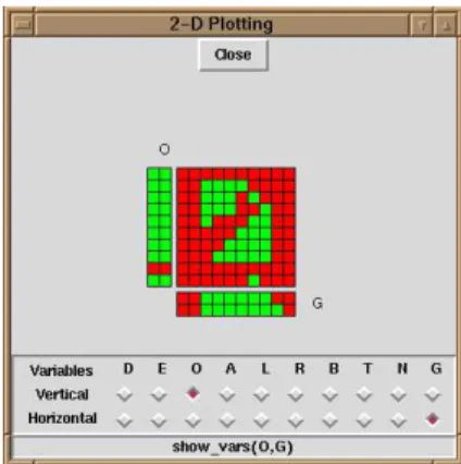
plot-Figure 15: Relating variables in VIFID
ting values of variables in a 2-D grid, which is equivalent to choosing values for one of them and looking at the al-lowed values for the other. This is shown in Figures 12, 13, and 14, where the variables are subject to the constraint C2. In each of these three figures we have represented a dif-ferent pair of variables. From these representations we can deduce that the values X = 3 and X = 6 are not feasible, regardless the values of Yand Z. It turns out also that the plots of XagainstYandXagainstZ(Figures 12 and 13) are identical. From this, one might guess that perhaps Y and Z have necessarily the same value, i.e., that the constraint Z = Yis enforced by the store. This possibility is discarded by Figure 14, in which we see that there are values of Zand Y which are not the same, and which in fact correspond to different values of X. Furthermore, the slope of the highlighted squares on the grid suggests that there is an inverse relationship between ZandY: incrementing one of them would presumably decrement the other.
Note that, in principle, more than two variables could be depicted at the same time: for example, for three variables a 3-D depiction of a “Lego object” made out of cubes could be used. Navigating through such a representation (for example, by means of rotations and virtual tours), does not pose implementation problems on the graphical side, but it may not necessarily give information as intuitively as the 2-D representation. The usefulness of such a 3-D (orn-D) representation is still a topic of further research. On the other hand, we have found it very useful to add to the 2-D representation the possibility of changing the value of one (or several) variables not plotted in the grid, and examine how this affects the values of the current domains of the variables in the grid. The ideas proposed are used in VIFID, a different snapshot of which is shown in Figure 15.
5
Abstraction
While representations which reflect all the data available in an execution can be acceptable (and even didactic) for “toy programs,” it is often the case that they result in too much data being displayed for larger programs. Even if an easy-to-understand depiction is provided, the amount of data can overwhelm the user with an unwanted level of detail, and with the burden of having to navigate through it. This can be alleviated byabstractingthe information presented. Here, “abstracting” refers to a process which allows a user to focus on interesting properties of the data available. Different abstraction levels and/or techniques can in principle be applied to any of the aforementioned graphical depictions, depending on which property we want to highlight.
Note that the depictions presented so far already incorporate some abstractions: for example, in the APT/VIFID node views only the relevant clause variables (or those indicated by the user) are shown, and when using VIFID standalone, the user selects the interesting variables and program points via the spypoints and the window controls. In what follows we will present several other ideas for
Figure 16: Exposing hidden parts of a tree Figure 17: Abstracting parts of a tree with color tagging performing abstraction, applied to the graphical representations we have discussed so far. Also, some new representations, which are not directly based on a refinement of others already presented, will be discussed.
6
Abstracting Control
The search tree discussed in Section 2 offers a good representation of the search (or enumeration) space being traversed. It also offers some degree of abstraction with respect to a classical search tree by reusing the tree nodes during backtracking. But it may still take up too much space and show too much detail to be useful in medium-sized computations, which can easily generate thousands of nodes.
The obvious way to cope with a very large number of objects (nodes and links) in the limited space provided by the screen is to use a canvas that is larger than the window and provide scrollbars to navigate through this canvas. However, this makes it difficult to see the “big picture”. An alternative is simply zooming the canvas to fit into the available space. This zooming can be made uniformly, or with a selective zooming which changes the compression ratio in different parts of the image. The former has the drawback that we lose the capacity to see the details of the execution when necessary. The latter seems more promising, since there might be parts of the tree which the user is not really interested in watching in detail (for example, because they belong to parts of the program which have been already tested, and (s)he is not interested in looking at them).
Examples of tools which compress part of the search tree are the VisAndOr and VISTA tools men-tioned before. This compression is performed automatically, at the points of greater density of objects— near the leaves. Those parts can also be zoomed out if a greater level of detail is needed. An alternative possibility to is to allow the user to slide virtual magnifying lenses which provide with a sort of fish-eye transformation and give both a global view (because the whole tree is shrunk to fit in a window) and a detailed view (because selected parts of the tree are zoomed out to greater detail). Providing at the same time a compressed view of the whole search tree, in which the area being zoomed is clearly depicted, can also help to locate the place we are looking at. An alternative solution providing these two views is provided in VisAndOr, where the canvas can be zoomed out, and at the same time the location of the current canvas view is given by a square in a reduced view of the whole picture.
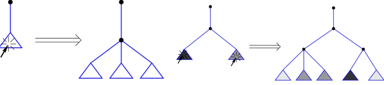
Another possibility to avoid cluttering up the display is to give the user a mean to hide parts of the tree, for example as done in the Oz explorer (Figure 16) [Sch97]. This actually allows for the selective exploration of the tree (i.e., in the cases where a call is being made to a predicate known to be correct, or whose performance has already been tested). Whereas this avoids having too many objects at a time, feedback on the relative sizes of the subtrees is lost. We propose to recover this information by tagging the collapsed subtrees with a mark which measures the relative “importance” of the subtrees. This importance can range from execution time to number of nodes, number of calls, number of added constraints, number of fixpoint steps in the solver, etc.: different measures lead to different abstractions. Possible tagging schemes are different shades of gray (which should be automatically re-scaled as subtrees are collapsed/expanded; see Figure 17 for an example) or raw numbers attached to the collapsed subtrees (indicating the concrete value measured under the subtree). This kind of tagged tree abstraction is currently being incorporated in the APT tree representation.
7
Abstracting Values
While the problem of the presence of a large number of variables can be solved, at least in part, by user selection of interesting variables, another problem remains: for variables with a large number of possible values representations such as those proposed in Section 3.1 can convey too much information to be really useful. These values may be too many to be clearly discerned, or to allow deducing any structure from the resulting pictures. At the limit, the screen resolution may be insufficient to assign a pixel to every single value in the domain, thus imposing an aliasing effect which would prevent faithfully reflecting the structure of the domain of the variable. This is easily solved by using the same techniques pointed out above for drawing big execution trees: a canvas that is larger than the window and scrollbars, providing means for zooming in and out, etc. Again, a “fish-eye” technique can be of help, giving the user the possibility of zooming precisely those parts which are more interesting, while at the same time trying to keep as much information as possible condensed in a limited space.
An alternative is to perform a more semantic “compaction” of parts of the domain. For example, this can be performed automatically by associating consecutive values in the domain of a variable to an interval (the smallest enclosing interval) and representing this interval by a reduced number of points. A coarser-level solution, perhaps complementary to the graphical representation is to present the domain of a variable simply as a number denoting, for example, the number of points in its current domain could, thus giving an indication of its degree of freedom. A similar approach can also be applied to interval variables, using the difference between the maximum and minimum values in its domain, or the total length of the intervals in its domain.
Another alternative for abstraction is to use an application-oriented filtering of the variable domains. For example, if some parts of the program are trusted to be correct, the effects of those parts in the constraint store can be masked out by removing them from the representation of the variables, thus leaving less values to be depicted. E.g., if a variable is known to take only odd values, the even values are simply filtered out and not shown in the representation. This filtering can be specified using the source language—in fact, the constraint which is to be abstracted should be the filter of the domain of the displayed variables. Note that this transformation of the domain cannot easily be completely automated: the debugger may not have any way of knowing which parts of the program are trusted and which are not, or which abstraction should be applied to a given problem. Thus, the user should indicate, with annotations in the program (assertions) or interactively, which constraints should be used to abstract the variable values. The actual reduction of the representation can be accomplished automatically given this information. Warnings could be issued by the debugger if the values discarded by the program do not correspond to those that the user (or the annotations in the program) want to remove: if this happens, a sort of “out of domain” condition can be raised. This condition does not mean necessarily that there is an error: the user may choose not to show uninteresting values which were not (yet) removed by the program.
8
Abstracting Constraints
As the number and complexity of constraints in programs grow, if we resort to visualizing them as relationships among variables (e.g., 2-D or 3-D grids plus sliding bars to assign values for other variables, as suggested in Section 4), we may end up with the same problems we had when trying to represent values of variables, since we are building on top of the corresponding representations. The solutions suggested for the case of representation of values are still valid (fish-eye view, abstraction of domains, . . . ), and can give an intuition of how a given variable relates to others. However, it is not always easy to deduce from them how variables are related to each other, due to the lack of accuracy (inherent to the abstraction process) in the representation of the variables themselves.
A different approach to abstracting the constraints in the store is to show them as a graph (see, e.g., [MR91] for a formal presentation of such a graph), where variables are represented as nodes, and nodes are linked iff the corresponding variables are related by a constraint (Figure 18)6. This representation
provides the programmer with an approximate understanding of the constraints are present in the solver
6This particular figure is only appropriate for binary relationships; constraints of higher arity would need
Figure 18: Constraints represented as a graph Figure 19: Bold frames represent definite values (but not exactlywhich constraints they are), after the possible partial solving and propagations per-formed up to that point. Moreover, since different solvers behave in different ways, this can provide hints about better ways of setting up constraints for a given program and constraint solver.
The topology of the graph can be used to decide whether a reorganization of the program is ad-vantageous; for example, if there are subsets of nodes in the graph with a high degree of connectivity, but those subsets are sparsely connected among them, it may be worth setting up the highly connected sections and making a (partial) enumeration early, to favor more local constraint propagation, and then link (i.e., set up constraints) the different regions, thus solving locally as many constraints as possible. In fact, identifying sparsely connected regions can be made in an almost automatic fashion by means of clustering algorithms. For this to be useful, a means of accessing the location in the program of the variables which appears depicted in the graph is needed. This can as well help discover unwanted constraints among variables—or the lack of them.
More information can be embedded in this graph representation. For example, weights in the links can represent various metrics related to aspects of the constraint store such as the number of times there has been propagation between two variables or the number of constraints relating them. The weights themselves need not be expressed as numbers attached to the edges, but can take instead a visual form: they can be expressed, for example, as different degrees of thickness or shades of color. Variables can also have a tag attached which gives visual feedback about interesting features. For example, the actual range of the variable, or the number of constraints (if it is not clear from the number of edges departing from it) it is involved in, or the number of times its domain has been updated.
The picture displayed can be animated and change as the solver proceeds. This can reflect, for example, propagation taking place between variables, or how the variables lose their links (constraints) with other variables as they acquire a definite value. In Figure 19 some variables became definite, and as a result the constraints between definite variables are not shown any more. The reason for doing so is that those constraints are not useful any longer. This reflects the idea of a system being progressively simplified. It may also help to visualize how backtracking is performed: when backtracking happens, either the links reappear (when a point where a variable became definite is backtracked over and a constraint is active again in the store), or they disappear (when the system backtracks past a point where a constraint was created).
Further filtering can be accomplished by selecting which types of constraints are to be represented (e.g, represent only “greater than” constraints, or certain constraints flagged in the program through annotations). This is quite similar to the domain filtering proposed in Section 7.
9
Conclusions
We have discussed techniques for visualizing program execution and data evolution in CLP. The graphical representations have been chosen based on the perceived needs of a programmer trying to analyze the behavior and characteristics of an execution. We have proposed solutions for the representation of program control, the runtime values of the variables, and the runtime constraints. In order to be able to deal with large executions, we have also discussed abstraction techniques. The proposed visualization solutions for visualizing control, variables, and constraints can be easily related, so that tools based on them can be used together in a complementary way. We have already implemented toolkits exemplifying combinations, such as the APT/VIFD combination presented, which we have found useful in practice.7 7Complementary approaches are being explored within the DISCIPL project by Cosytec, INRIA and PrologIA.
References
[AM94] K. R. Apt and E. Marchiori. Reasoning about Prolog programs: from modes through types to assertions. Formal Aspects of Computing, 6(6):743–765, 1994.
[AS97] A. Aggoun and H. Simonis. Search Tree Visualization. Technical Report D.WP1.1.M1.1-2, COSYTEC, June 1997. In the ESPRIT LTR Project 22352 DiSCiPl.
[BDD+97] F. Bueno, P. Deransart, W. Drabent, G. Ferrand, M. Hermenegildo, J. Maluszynski, and
G. Puebla. On the Role of Semantic Approximations in Validation and Diagnosis of Con-straint Logic Programs. In Proc. of the 3rd. Int’l Workshop on Automated Debugging– AADEBUG’97, pages 155–170, Link¨oping, Sweden, May 1997. U. of Link¨oping Press. [BDM97] R. Baecker, C. DiGiano, and A. Marcus. Software Visualization for Debugging.
Communi-cations of the ACM, 40(4):44–54, April 1997.
[Byr80] L. Byrd. Understanding the Control Flow of Prolog Programs. In S.-A. T¨arnlund, editor,
Workshop on Logic Programming, Debrecen, 1980.
[CGH93] M. Carro, L. G´omez, and M. Hermenegildo. Some Paradigms for Visualizing Parallel Exe-cution of Logic Programs. In 1993 International Conference on Logic Programming, pages 184–201. MIT Press, June 1993.
[DC93] Daniel Diaz and Philippe Codognet. A minimal extension of the WAM for clp(FD). In David S. Warren, editor, Proceedings of the Tenth International Conference on Logic Pro-gramming, pages 774–790, Budapest, Hungary, 1993. The MIT Press.
[DN94] Mireille Ducass´e and Jacques Noy´e. Logic Programming Environments: Dynamic Program Analysis and Debugging. The Journal of Logic Programming, 19 & 20:351–384, May 1994. [DNTM89] W. Drabent, S. Nadjm-Tehrani, and J. Maluszynski. Algorithmic debugging with assertions.
In H. Abramson and M.H.Rogers, editors,Meta-programming in Logic Programming, pages 501–522. MIT Press, 1989.
[Duc92] Mireille Ducass´e. A General Query Mechanism Based on Prolog. In M. Bruynooghe and M. Wirsing, editors, International Symposium on Programming Language Implementation and Logic Programming, PLILP’92, volume 631 of LNCS, pages 400–414. Springer-Verlag, 1992.
[EB88] M. Eisenstadt and M. Brayshaw. The Transparent Prolog Machine (TPM): An Execution Model and Graphical Debugger for Logic Programming. Journal of Logic Programming, 5(4), 1988.
[Fab97] Massimo Fabris. CP Debugging Needs. Technical report, ICON s.r.l., April 1997. ESPRIT LTR Project 22352 DiSCiPl deliverable D.WP1.1.M1.1.
[Fer94] J.M. Fern´andez. Depuraci´on declarativa para BABEL. Master’s thesis, School of Computer Science, Technical University of Madrid, October 1994. In Spanish.
[JM94] J. Jaffar and M.J. Maher. Constraint Logic Programming: A Survey. Journal of Logic Programming, 19/20:503–581, 1994.
[Kah96] K. Kahn. Drawing on Napkins, Video-game Animation, and Other ways to program Com-puters. Communications of the ACM, 39(8):49–59, August 1996.
[Lue97] A. L´opez Luengo. Apt: implementaci´on de un visualizador gr´afico de la ejecuci´on de progra-mas l´ogicos. Master’s thesis, Technical University of Madrid, School of Computer Science, E-28660, Boadilla del Monte, Madrid, Spain, October 1997. In Spanish.
[Mei96] M. Meier. Grace User Manual, 1996. Available at
http://www.ecrc.de/eclipse/html/grace/grace.html.
[Mic97] Sun Microsystems. Animated Sorting Algorithms, 1997. Available at http://java.sun.com/applets/.
[MR91] U. Montanari and F. Rossi. True-concurrency in Concurrent Constraint Programming. In V. Saraswat and K. Ueda, editors,Proceedings of the 1991 International Symposium on Logic Programming, pages 694–716, San Diego, USA, 1991. The MIT Press.
[Sch97] Christian Schulte. Oz explorer: A visual constraint programming tool. In Lee Naish, editor,
ICLP’97. MIT Press, July 1997.
[Swe95] Swedish Institute of Computer Science, P.O. Box 1263, S-16313 Spanga, Sweden. Sicstus Prolog V3.0 User’s Manual, 1995.
[Tic92] Evan Tick. Visualizing Parallel Logic Programming with VISTA. InInternational Confer-ence on Fifth Generation Computer Systems, pages 934–942. Tokio, ICOT, June 1992.