University of Colorado, Boulder
CU Scholar
Undergraduate Honors Theses
Honors Program
Spring 2011
Multivariate Nonparametric Estimation of Value at
Risk and Expected Shortfall for Nonlinear Returns
Using Extreme Value Theory
Ryan Brauchler
University of Colorado Boulder
Follow this and additional works at:
http://scholar.colorado.edu/honr_theses
Recommended Citation
Brauchler, Ryan, "Multivariate Nonparametric Estimation of Value at Risk and Expected Shortfall for Nonlinear Returns Using Extreme Value Theory" (2011).Undergraduate Honors Theses.Paper 614.
Multivariate Nonparametric Estimation of Value at Risk and
Expected Shortfall for Nonlinear Returns Using Extreme Value
Theory
By, Ryan Brauchler
Primary Advisor: Professor Carlos Martins-Filho, Economics Department Honors Committee Member: Professor Terra McKinnish, Economics Department
Outside Reviewer: Professor Karl Gustafson, Math Department
Undergraduate Departmental Honors Thesis Department of Economics
University of Colorado at Boulder November 4, 2011
Multivariate Nonparametric Estimation of Value at Risk and
Expected Shortfall for Nonlinear Returns Using Extreme Value
Theory
∗Abstract
The catastrophic failures of risk management systems in 2008 bring to the forefront the need for accurate and flexible estimators of market risk. Despite advances in the theory and practice of evaluating risk, existing measures are notoriously poor predictors of loss in high-quantile events. To extend the research concerned with modeling extreme value events, we utilize extreme value theory (EVT) to propose a multivariate estimation procedure for value-at-risk (VaR) and expected shortfall (ES) for conditional distributions of a time series of returns on a financial asset. Our approach extends the local linear estimator of conditional mean and volatility used in the condi-tional heteroskedastic autoregressive nonlinear (CHARN) model proposed by Martins-Filho and Yao (2006) by incorporating an exogenous time series resembling returns on the S&P 500 from Jan-uary 1950 through September 2011. In combination with EVT, this model estimates the quantiles of the conditional distribution and subsequently the one-day forecasted VaR and ES. We examine the finite sample properties of our method and contrast them with the popular Gaussian GARCH estimator in an extensive Monte Carlo simulation. The method we propose generally outperforms the Gaussian GARCH estimator, particularly in samples greater than 1000. Our results provide evi-dence of the effect of the curse of dimensionality, which arises because we include a second regressor.
Keywords and phrases. Value at risk, expected shortfall, market risk, nonparametric estimation, extreme value theory, L-moments, nonlinear modeling, Monte Carlo
JEL Classifications. C01, C14, C58, G01, G17, G32.
AMS-MS Classification. 62G05, 62G08, 62G32.
∗The author would like to thank Carlos Martins-Filho for his invaluable contributions, suggestions, and teachings during the research process. The author would also like to thank David Keyes, of the University of Colorado Math Department, for his revisions and commentary.
Contents
1 Introduction 1
2 Literature Review 3
2.1 Data Generating Process . . . 3
2.2 Definitions of VaR and ES . . . 5
2.3 L-Moments and Maximum Likelihood Estimation . . . 6
2.4 Local Polynomial Regression . . . 11
2.5 Extreme Value Theory . . . 11
2.6 Properties of Financial Return Series and Modeling . . . 12
2.6.1 Properties of Financial Time Series . . . 12
2.6.2 Modeling Financial Returns . . . 15
3 VaR and ES Estimation Method 20 3.1 Estimation of ˆmand ˆσ2 . . . 20
3.2 Estimation ofβ andψ Using L-moments . . . 23
3.3 Estimation of VaR and ES . . . 24
3.4 Alternative First Stage Estimation Procedures . . . 25
4 Monte Carlo Simulation 26 5 Results 28 5.1 General Relative Performance . . . 29
5.2 Ceteris Paribus Relationships . . . 31
6 Conclusion 33
A Appendix A - Tables and Graphs 35
1
Introduction
“There is always a well-known solution to every human problem - neat, plausible, and wrong.” -H.L. Mencken
After myriad instances of catastrophic failure of risk management systems during the financial crisis of 2008, accurate measurement of the degree to which firms are exposed to market risk became a central concern among internal risk management departments, regulators, and investors. Recent financial reform measures including Basel III, the Volcker Rule, and the sweeping Dodd-Frank Act exemplify the gravity granted to reliably mitigating and accurately measuring risk. Accurate estimation of the market risk to which financial institutions are exposed gives policymakers and portfolio managers insight into capital adequacy requirements which they can use to make better-informed decisions. This paper aims to construct alternative estimators for value-at-risk (VaR) and expected shortfall (ES) to outperform those existing in the literature and provide risk managers and legislators with a better predictor of performance in extreme scenarios, thereby helping forecast, mitigate, and manage risk.
The challenge of synthetically measuring the market risk faced by a firm with a single figure gave rise to VaR (JPMorgan (1996)) and ES (Artzner et al. (1999)). VaR estimates the maximum financial loss on a portfolio over a given time horizon (usually 24 hours) under a specified confidence level (Jorion (2001)). By contrast, ES, also known as Conditional VaR or TailVaR, considers the expected value of all losses exceeding a quantile prescribed by a level of confidence over a specified time interval (Acerbi and Tasche (2002)). Statistically, VaR is a quantile and ES is the expected value of a random variable exceeding a quantile. Since their conception, VaR and ES have been both praised and criticized, and many alternative measures have been proposed in the literature. Though VaR and ES are often adequate risk measures, they are notoriously difficult to estimate
for high order quantiles, which is an issue this paper aims to address.
The model proposed in this paper modifies the local linear estimator of conditional mean and volatility used in the conditional heteroskedastic autoregressive nonlinear (CHARN) model proposed by Martins-Filho and Yao (2006) for estimating quantiles of conditional distributions. Hereafter, their original model will be termed the MFY Model. This paper makes two contributions to the literature on VaR and ES estimation. First, we propose the inclusion of an exogenous explanatory variable in the conditional location scale model used in estimation of VaR and ES. Specifically, we consider adding an exogenous series modeled after the returns distribution of the S&P 500 equity index from January 3, 1950 through September 30, 2011. This stochastic variable will act as a control for factors that exhibit significant collinearity with the primary time series. Second, we conduct an extensive Monte Carlo simulation to examine the finite sample properties of our estimator. The Monte Carlo compares the relative performance of our model against the ever popular Gaussian Generalized Autoregressive Conditionally Heteroskedastic (GARCH) model of Bollerslev (1986). Our Monte Carlo study considers several data generating processes (DGPs) that exhibit the empirical properties of financial time series, including “asymmetric conditional volatility, leptokurdicity, infinite past memory and asymmetry of conditional return distributions” (Martins-Filho and Yao (2006)). Performance is measured by root mean squared error (RMSE) and bias.
The remainder of this paper is organized as follows: Section 2 provides a discussion of the statis-tical methods used in our estimation, EVT, properties of financial assets’ returns, and approaches to modeling the returns and volatility of financial assets. Section 3 offers a detailed treatment of the VaR and ES estimation methods we use. Section 4 outlines the design of the Monte Carlo sim-ulation. Section 5 summarizes the results of the Monte Carlo. Section 6 contains a brief conclusion
and suggestions for further research.
2
Literature Review
This literature review will focus on the statistical methods used in our estimation procedure for VaR and ES. Since the procedure here modifies the existing MFY procedure and is therefore pre-determined, we limit the discussion of previously proposed VaR and ES estimation procedures to ARMA and GARCH variants of first stage estimators. Instead, this section focuses on the math-ematical concepts and methods that are essential to understanding the estimation procedure used in our model.
2.1
Data Generating Process
We first define the data generating process used as the basis for the Monte Carlo simulation pre-sented in section 4. It is this process that underlies all the data we use. The DGP that we consider is a modified version of the nonparametric GARCH model proposed by Hafner (1998), studied by Carroll et al. (2002), and utilized by Martins-Filho and Yao (2006). Take{Yt} to be a stochastic
process of log-returns on a financial asset whereE(Yt|Yt−1, Dt−1) = 0 andE(Yt2|Yt−1, Dt−1) =σt2
and whereDt−1 represents lagged returns of an exogenous variable. For our purposes, the
exoge-nous variable mimics the returns distribution of the S&P 500 since January 3, 1950. We assume the returns process evolves as,
Yt=σtt fort= 1,2, ... (2.1)
σ2t =g(Yt−1, Dt−1) +γσt2−1 (2.2)
where g(x) is a positive, twice continuously differentiable function and 0< γ < 1 is a weighting parameter for the one-period lagged volatility. tis a sequence of IID random variables exhibiting
and a discussion of the skewed Student-t density, consult Hansen (1994). The skewed Student-t’s PDF, normalized to haveE(t) = 0 and V ar(t) = 1, is given by
f(x;v, λ) = bc 1 + 1 v−2 bx+a 1 +λ 2!(−v+1)/2 forx≥ −a/b bc 1 + 1 v−2 bx+a 1−λ 2!(−v+1)/2 forx≤ −a/b (2.3) wherec≡ Γ v+1 2 Γ v 2 p π(v−2), a≡4λc v−2 v−1, b≡ p
1 + 3λ2−a2. The parametervrepresents degrees
of freedom andλis the skewness parameter. Note that whenλ= 0, the skewed Student-t becomes a symmetric standardized Student-t.
Patton (2004) derived the VaR (α-quantile) for the skewed Student-t distributed sequence,y,t,
given by q(α) = 1−λ b r v−2 v F −1 s α 1−λ, v −a b for 0< α < 1−λ 2 1 +λ b r v−2 v F −1 s 0.5 + 1 1 +λ α−1−λ 2 , v −a b for 1−λ 2 ≤α <1 (2.4)
whereFs−1 is the inverse CDF of a random variable with a symmetric Student-t distribution with
vdegrees of freedom and αconfidence level.
Martins-Filho and Yao (2006) derived the Expected Shortfall for the skewed Student-t dis-tributed sequence,t, by E(t|t> q(α)) = (1−F(q(α), v))−1 c(1 +λ)2 b v−2 v−1 β(v−1)/2 −(1 +λ)a b 1−Fs bq (α) +a 1 +λ r v v−2, v (2.5) whereβ = cos arctan bq (α) +a (1 +λ)√v−2 2
,Fs is the CDF of a random variable with a
sym-metric Student-t distribution, v degrees of freedom, andα confidence level; andF is the CDF of a random variable with a skewed Student-t distribution andv degrees of freedom with skewness parameterλ.
The above DGP exhibits many of the stylized regularities observed in returns on financial assets, including asymmetric conditional variance with greater volatility for large negative returns and less volatility for positive returns (Hafner (1998)), long memory in volatility, significant collinearity with exogenous variables, conditional skewness (Patton (2004); Chen (2001); Ait-Sahalia and Brandt (2001)), leptokurdicity (Tauchen (2001); Andreou et al. (2001)), and nonlinear temporal dependence (Martins-Filho and Yao (2006)). The DGP is therefore able to adequately demonstrate most of the properties of financial returns and provides a useful approximation for our Monte Carlo.
2.2
Definitions of VaR and ES
Using the conventions of Martins-Filho and Yao (2006), VaR is formally defined as follows. Let{Yt}
be a stochastic process representing a sequence of returns on a given financial asset, with discrete-time indext. Let the unknown conditional distribution ofYtbe denoted byFt, which is absolutely
continuous. Ftis conditioned on a sequence of lagged realizations, given as,{Yt−k}1≤k≤M, for some M ≥1. For 0<α<1, theα-VaR ofYtis the α-quantile of the conditional CDF,Ft. We denote it
byFt−1(α|{Yt−k}1≤k≤M) and assume that
Ft−1(α|{Yt−k}1≤k≤M) =µt+σtq(α) (2.6)
Expressed informally, VaR gives the maximum financial loss on a portfolio over a given time horizon that will happen with probability not exceeding 1−α.
Expected shortfall is defined asEFy
t(Yt), which denotes the expected value taken with respect
to Fty, the truncated distribution defined such that Yt>y where y is a specified loss threshold.
Whenever the threshold y is taken to be α-VaR, we refer to α-ES. Expressed mathematically, expected shortfall is given as in Martins-Filho and Yao (2006) as,
Informally, ES gives the expected loss on a financial asset or portfolio given that losses exceed a specified quantile.
Accurately estimating VaR and ES depends crucially on the ability to estimate the tails of the probability density function (PDF)ftassociated with the cumulative distribution function (CDF) Ft. Traditional methods of tail estimation are insufficient to accurately model tail events since
the vast majority of realizations of the relevant random variable will take values near the center of the distribution (Diebold et al. (1993)). Extreme value theory (EVT) attempts to model the probability distributions of highly unlikely occurrences by approximating only the tails offtvia an
appropriately defined parametric density function. We discuss this further in section 2.5.
2.3
L-Moments and Maximum Likelihood Estimation
L-moments estimators are defined as summary statistics for probability distributions and data samples (IBM Corporation (2003)). L-moments are analogous to traditional moments in that they provide measures of location, dispersion, skewness, kurtosis, and higher-order moments for any probability distribution. L-moment estimators are computed using linear combinations of the ordered values of the data sample (Hosking (1990)).
Hosking (1990) outlined the following advantages of L-moments over conventional statistical moments :
• The probability distribution of the data sample must possess a finite mean, but need not possess any finite higher order moments. A distribution can be characterized uniquely by its L-moments as long as this is true (Martins-Filho and Yao (2006)).
• Sample L-moment ratios (analogous to standardized moments) can assume any value possible within the corresponding population.
• Asymptotic approximations of sampling distributions are better for L-moments than conven-tional moments (IBM Corporation (2003)).
• As a result of their definition as linear combinations of the data, L-moments are less susceptible to the effects of sampling variability and outliers in the data sample (Royston (1992)).
• L-moments allow for better inferences to be made from small samples about the probability distribution underlying the data sample.
• L-moments outperform ML estimators on an MSE basis in finite samples (Martins-Filho and Yao (2006); Hosking et al. (1985); Hosking and Wallis (1987)).
For a detailed treatment of the mathematical properties underlying the above claims, consult Hosk-ing (1990); HoskHosk-ing and Wallis (1997); Martins-Filho and Yao (2006).
We formally define L-moments both generally and for finite samples as they are presented in Martins-Filho and Yao (2006). Letbe a random variable representing residuals and let F be its
CDF. Letα∈(0,1) and define q(α) as its quantile. Forr∈N, therthL-moment of is defined
as, λr= Z 1 0 q(α)Pr−1(α)dα (2.8) wherePr(α) = r X k=0 pr,kαkandpr,k= (−1)r−k(r+k)! (k!)2(r−k)! . Pr(α) is ther
thshifted Legendre orthogonal
polynomial. Conversely, conventional moments are defined byµr=
Z 1
0
q(α)rdα, whereµr is the
general term for therthconventional moment.
L-moments can be used to estimate a finite number of parameters θ ∈ Θ, which characterize a member of a family of distributions. For p ∈ N, let {F(θ) : θ ∈ Θ ⊂ Rp} be a family of
distributions known up toθ parameters. We denote our collection of residuals by{t}Tt=1 where
implies thatθ may be expressed as a function ofλr. If we are able to estimate ˆλr from {t}Tt=1,
then we may also estimate ˆθ(ˆλ1,λˆ2, ...). By equation (2.8),λr+1=
r X k=0 pr,kβk forr= 0,1, ...where βk = Z 1 0
q(α)αkdα for r= 0,1, ...are the probability weighted moments. For {t}Tt=1, we define
(k) as the kth smallest element in the sample such that (1) ≤ (2) ≤ ... ≤ (T). As defined in
Martins-Filho and Yao (2006), an unbiased estimator ofβk is
ˆ βk = 1 T T X j=k+1 (j−1)(j−2)...(j−k) (T−1)(T−2)...(T−k)(j) (2.9) and we define ˆλr+1= r X k=0 pr,kβˆk forr= 0,1, ..., T−1.
One can also consider a different calculation methodology for L-moments in finite samples, as given by Wang (1997). Wang (1997) showed that the first four L-moments in a finite sample of datax(t) sorted into its order statistics, denotedλ1, λ2, λ3, andλ4, can be expressed by,
λ1= T 1 −1 T X t=1 x(t) = 1 T T X t=1 x(t) (2.10) λ2= 1 2 T 2 −1 T X t=1 t−1 1 − T−t 1 x(t) = 1 T(T−1) T X t=1 (2t−T −1)x(t) (2.11) λ3= 1 3 T 3 −1 T X t=1 t−1 2 −2 t−1 1 T−t 1 − T−t 2 x(t) = 1 T(T−1)(T −2) T X t=1 [(t−1)(t−2)−4(t−1)(T−t) + (T −t)(T−t−1)]x(t) (2.12) λ4= 1 4 T 4 −1 T X t=1 t−1 3 −3 t−1 2 T−t 1 −3 t−1 1 T−t 2 − T−t 3 x(t) = 1 T(T−1)(T −2)(T−3) T X t=1 [(t−1)(t−2)(t−3)−9(t−1)(t−2)(T−t) +9(t−1)(T−t)(T−t−1)−(T−t)(T−t−1)(T−t−2)]x(t) (2.13)
where a
b
is the binomial coefficient. We utilize the simplified versions of the first two L-moments in our procedure.
Assuming it exists, the first L-moment is a measure of the location of a distribution. The first L-moment is equivalent to the conventional first moment (i.e. λ1 = µ1). λ2 is a measure
of the dispersion of the distribution and is a scalar multiple of the expectation of Gini’s mean difference statistic.1 λ2places smaller weights on the differences between estimates and realizations
of the random variable and as such, it produces a measure of scale not equivalent to conventional variance (Hosking (1990)). Higher order moments are characterized as L-moment ratios, where forr ∈N, τr =
λr λ2
. Therefore, L-skewness, the third moment, is denoted τ3 ≡
λ3
λ2
. Ifµ1 exists,
−1 < τ3 < 1 with τ3 = 0 for symmetric distributions (Hosking (1989)). This means that
L-skewness is bounded and therefore less sensitive to extreme values in the tails of the distribution than conventional, unbounded skewness. A similar result is observed by Oja (1981) for L-kurtosis,
τ4, where−1< τ4<1. L-kurtosis is also bounded and less sensitive to outliers in the distribution.
These characteristics of L-moments are desirable for modeling the statistical regularities present in financial time series, which are discussed in detail in section 2.6.
Our assumption that the tails of the distribution may be approximated by a generalized pareto distribution (discussed later) may be restrictive in MLE. If the tail is actually not prescribed by a GPD and the ML estimators are calculated under the assumption that it is, then the ML estimators may be biased, while the non-parametric L-moments may provide better estimates. Additionally, in “highly nonlinear dynamic models with fat tails and latent variables, asymptotic efficiency of the maximum likelihood (ML) estimator is not always warranted” (Andersen et al. (2009)). In fact,
1Gini’s mean difference statistic is a measure of statistical dispersion that considers the average absolute difference
between two realizations of a random variable drawn from a specified probability distribution. Providednrealizations of some random variablex, the mean difference is given by,M D=
PT i=1
PT
j=1|xi−xj| T(T−1) .
in nonstationary cases such as financial time series, the ML estimates are no longer asymptotically normal (Chan and Wei (1988); Phillips and Yu (2009)).
Maximum likelihood estimation (MLE) is the most popular method used by econometricians and statisticians to estimate the parameters of a model. Generally, for a set of data with an underlying probability distribution, MLE selects values for the parameters of the model that produce the distribution most likely to have generated the observed data. If the data are independent and identically distributed (IID), it is possible to express the joint density functionf(y1, ..., yT|θ) where y1, ..., yT are the observed values of the data andθis a vector of parameters of the data. The joint
density is therefore given byf(y1, ..., yT|θ) =f1(y1|θ)×...×fT(yT|θ). If the data exhibit dependence,
we may define the conditional joint density as f(y1, ..., yT|θ) = f(yT|yT−1, yT−2, ..., y1, θ)×...×
f(y1|θ). Many practitioners use MLE to estimate model parameters because ML estimators exhibit
several attractive asymptotic properties in stationary dynamic models (Wald (1949); Andersen et al. (2009); Hall and Heyde (1980); Billingsley (1961); Dacunha-Castelle and Florens-Zmirou (1986)), namely:
• Consistency - As the number of observations,T, grows, a sequence of ML estimators converges in probability to the true value (ˆθmle
p
−→θ0)
• Asymptotic normality - As T grows, the ML estimator assumes an asymptotically normal distribution when suitably standardized (√T(ˆθmle−θ0)
d
−→N(0, I−1)) whereI is the Fisher Information matrix. For largeT, ML estimators achieve the Cramer-Rao lower bound, mean-ing that there exists no asymptotically unbiased estimator with lower mean squared error (MSE).
Note that all of the above properties hold asymptotically. For the purposes of our paper, we seek to uncover the finite sample properties of our estimators for VaR and ES since all applied financial work
is conducted using finite samples. As such, we employ L-moments estimation of the parameters of our DGP.
2.4
Local Polynomial Regression
Local polynomial regression is a nonparametric nonlinear estimation procedure that fits a regression function to a data series in a piecewise manner, considering only partial windows of the sample data at a time. We define local polynomial regression as in Fan (1992). Consider a sequence (X1, Y1), ...,(XT, YT) of random variables from a population with unknown density f(x, y). The
marginal density ofX is thereforefX(x). The regression functionm(x) is a conditional expectation
forY, denotedm(x) =E(Yt|Xt=x)∀t. The conditional variance is given asσ2(x) =V ar(Yt|Xt= x)∀t.
Martins-Filho and Saraiva (2011) define local polynomial smoothers for univariate regressions as follows. Let apth order local polynomial regression estimator for conditional expectation ofYt
given regressorXtdenoted by ˆm(x), be given by,
ˆ m(x)≡(ˆaT0(x;h), ...,ˆaT p(x;h)) = argmin a0,...,ap T X t=1 Yt− p X j=0 aj(Xt−x)j 2 K X t−x h (2.14)
whereK is a kernel estimator with optimally determined bandwidthhand vanishing higher-order moments. Higher order estimators for m(x) are rarely used in practice because as the order p
increases, the necessary assumption of p-times differentiability may become restrictive. For our first stage estimation procedure, we utilize local linear regression, which is the special case of equation (2.14) wherep= 1.
2.5
Extreme Value Theory
Extreme value theory (EVT) is a field of statistics concerned with modeling maxima and extreme values of random variables. There are two traditional methods by which extreme values are modeled.
The cornerstone of EVT is the Fisher-Tippett-Gnedenko Theorem, which states that the maximum of a sample of IID random variables converges in distribution to one of only three possible families of distributions: the Gumbel distribution, the Frechet distribution, or the reverse Weibull distribution (Fisher and Tippett (1928)). Gnedenko (1943) later proved the necessary and sufficient conditions for which this result holds. These distributions are special cases of the generalized extreme value (GEV) distribution (McFadden (1978)).
An interesting result was obtained by Pickands (1975), which states that the distribution of the exceedances (residuals) of a random variable,, over a specified threshold,u, can be approximated by a generalized pareto distribution (GPD) with mean zero, providedF belong to the domain of
attraction of a Gumbel, Frechet, or reverse Weibull distribution. Letbe a stochastic variable with shape parameterψand scale parameter β. The CDF of the GPD is given by,
F(;ψ, β) = 1− 1 +ψ β −1/ψ , ∈D
and the PDF is given by,
f(;ψ, β) = 1 β 1 +ψ β −(1+ψ1)
whereD= [0,∞) ifψ≥0 andD= [0,−β/ψ] ifψ <0. Our estimation procedure makes use of this result to approximate only the tails, or extreme values, of the distribution underlying our data.
2.6
Properties of Financial Return Series and Modeling
2.6.1 Properties of Financial Time Series
Asymmetry of the conditional return distribution - Returns on financial assets exhibit
leptokurtosis, meaning that their probability distributions possess ‘fat tails.’ From a modeling perspective, fat tails imply that there is a greater probability of experiencing large gains or losses than under the assumption of normality. As such, modeling procedures employing an assumption
of normality ignore the significant impact of higher-order moments on their estimation, particularly in tail estimation.
Financial returns also exhibit negative conditional skewness, meaning a larger portion of the probability density function takes values below the median than a symmetric distribution would predict. With respect to returns modeling, ignoring skewness will overestimate the likelihood of large positive gains while also underestimating the likelihood of large losses. For more thorough characterizations of these results, see Tauchen (2001); Andreou et al. (2001); Hafner (1998); Ait-Sahalia and Brandt (2001); Chen (2001); Patton (2004); Gallant and Tauchen (1989), and Bodie et al. (2009).
Asymmetric conditional volatility - Literature suggests that volatility in returns of a
fi-nancial asset tends to be greater in a downward trend than in an upward trend. Essentially, when losing value, we tend to see more volatility than when gaining value. This property has particularly salient applications to event studies, such as those dealing with the impact of news on returns, in which negative news releases typically have a greater impact than positive releases (Engle and Ng (1993)). One need only examine the historical record to see far greater volatility in periods of reces-sion and economic contraction than in periods of expanreces-sion. For more thorough characterizations of this result, see Kroner and Ng (1998); Black (1976); Pagan and Schwert (1990); Engle and Ng (1993), and Hafner (1998).
Long memory in returns - The literature suggests that financial time series exhibit long
memory in returns, meaning returns exhibit high autocorrelations with prior returns. This result essentially negates the assumption that financial return series are independent. Characteristics of the markets or assets being analyzed do have a significant impact on long memory properties. Limam (2003) found, for example, that long memory tends to exist more in thin markets. Long
memory in returns is observed much less often in very liquid markets.
Specifically, financial time series are characterized by nonlinear temporal dependence (Martins-Filho and Yao (2006)). Correlogram plots for various financial time series show a distinct hyperbolic decay in correlation that is well-described by a fractionally-integrated process (Andersen et al. (2009)). Similar results are found for currencies (Andersen and Bollerslev (1997, 1998); Andersen et al. (2001); Cheung (1993); Zumbach (2004)), equities (Andersen et al. (2001); Areal and Taylor (2002); Deo et al. (2006); Martens (2002)), and bond yields (Andersen and Benzoni (2010)). For more results concerning long memory in returns, see Breidt et al. (1998); Engle and Lee (1999); Goetzmann (1993); Nawrocki (1993), and Huang and Yang (1999).2
Volatility clustering -Volatility clustering means that periods of high volatility tend to follow
periods of high volatility, while periods of low volatility tend to follow periods of low volatility. This stylized fact is one of the most persistent and is most consistently supported in the literature. Volatility persistence is the econometric analog to Newton’s First Law of Motion: an object at rest tends to remain at rest and an object in motion tends to remain in motion. This property is also known as volatility persistence, long memory in volatility, or serial correlation in volatility. For more thorough characterizations of these results, see Fan and Yao (1998); Bollerslev et al. (1992); Bollerslev (1986); Mandelbrot (1963); Fama (1965); Poterba and Summers (1986); Engle and Mustafa (1992), and Milhoj (1985).
Leverage effect - A reduction in the equity value of a financial asset would raise its
debt-to-equity ratio, implying greater riskiness of the asset in the form of an increase in future volatility. As a result, future volatility is negatively related to the current return on a financial asset. This property is known as the leverage effect. For more information on the leverage effect, consult Black
2For papers which find do not find support for the property of long memory in returns, see Lo (1991); Lobato
(1976); Christie (1982); Kupiec (1989); Chen (2001); Ding et al. (1993); Hafner (1998); Engle and Patton (2001); Patton (2004), and Gallant et al. (1992).
2.6.2 Modeling Financial Returns
This subsection provides a brief discussion of the statistical approaches used to model returns on financial assets. It serves as a historical account of the developments leading to the modeling techniques employed both in recent literature and this paper. Note that the following discussion is by no means exhaustive or comprehensive. For more thorough treatments of time series modeling, see Andersen et al. (2009); Terasvirta (2008).
ARMA Models - Autoregressive Moving Average (ARMA) models are a class of time series
models used to analyze and forecast stationary stochastic time indexed variables. We let {Yt} be
a univariate covariance stationary time series. The property of stationarity requires that E[Yt] is
independent of the time indextand thatCov(Yt, Yt+h) is finite and depends only on the lag,h, not
the position in the series. We define ARMA models as in Holan et al. (2010). The series {Yt} is
an ARMA series with autoregressive orderp≥0 and moving average orderq≥0 if it is stationary and a solution to the equation given by,
Yt=α+ p X i=1 φiYt−i+ q X i=1 θit−i+t (2.15)
whereαis some intercept constant and{t}is a mean zero white noise (IID) process of residuals with V ar(t)≡σt2. The parameters of the ARMA model are estimated by MLE, Method of Moments, or
OLS regression. For clarity, autoregressive terms are previous realizations of the regressand, while the moving average terms are past realizations of error terms, which are typically assumed to follow a prescribed distribution, Gaussian or otherwise.
ARMA models may be generalized to include the effects of other exogenous variables, as is the case in the autoregressive moving average with exogenous inputs (ARMAX) model (Peng et al.
(2001)). The ARMAX model is defined as, Yt=α+ p X i=1 φiYt−i+ q X i=1 θit−i+ b X i=1 ηidt−i+t (2.16)
where{dt}is a exogenous time series andη1, ..., ηbare the coefficients of{dt}. tandαare defined
as above. This is the alternative first stage estimation approach used in our Monte Carlo simulation. Even more general is the nonlinear autoregressive exogenous (NARX) model presented by Leon-taritis and Billings (1985a,b), which is given by,
Yt=m(Yt−1, Yt−2, ..., dt, dt−1, dt−2, ...) +t (2.17)
wheret remains the white noise error term and mis some nonlinear function estimated through
nonlinear regression techniques or machine learning algorithms.
ARCH/GARCH Models3-The class of autoregressive conditionally heteroskedastic (ARCH)
models arose to address the property of serial correlation and non-stationarity in asset returns. En-gle (1982) introduced the ARCH(q) model where conditional variance is written as a distributed lag ofqpast squared innovations,
σ2t =α+
q
X
i=1
βi2t−i (2.18)
where α is the intercept parameter and the βi are the coefficients on the lagged residuals, t−i,
which are assumed to be distributed N(0, σ2). For the conditional volatility to be positive, note
that theαandβi coefficients must also be positive.
Bollerslev (1986) later proposed the generalized autoregressive conditionally heteroskedastic (GARCH) model to reduce the number ofβicoefficients while still capturing persistence in volatility.
The GARCH(p, q) model, wherepis the order of the autoregressive lags on theσt2−i terms andqis
3For all the GARCH definitions, we definet=σtztwhereσtis the standard deviation of the data andztis an
the order of the moving average lags on the2t−i terms, is given as, σ2t =α+ p X i=1 ωiσt2−i+ q X i=1 βi2t−i (2.19)
whereαis the intercept parameter, theωis are the coefficients on the autoregressive lags, and the βis are the coefficients on the moving average lags. Though the GARCH model is also a weighted
average of past squared residuals, it is different because it contains declining weights that never equal zero. This characteristic captures the persistent memory documented in asset returns. Note that “GARCH models are mean reverting and conditionally heteroskedastic, but have a common unconditional variance” (Sheth and Kim (2003)).
In 1993, Engle and Ng introduced the nonlinear GARCH (NGARCH) model to capture asym-metry. NGARCH is a special case of the GARCH(1,1) model, given by,
σ2t =α+β(t−1−θσt−1)2+ωσt2−1 (2.20)
whereβ, ω≥0 andα >0. NGARCH models demonstrate the leverage effect whenθ is estimated to be positive (Posedel (2006)).
The exponential GARCH (EGARCH) model proposed by Nelson (1990) is a nonlinear expansion of the traditional GARCH model. Nelson definedσt2 as an asymmetric function of past residuals,
t, given by, ln(σ2t) =α0+ p X i=1 αi(φzt−i+γ(|zt−i| −E|zt−i|)) + q X i=1 βiln(σt2−i) (2.21)
where the error process zt is assumed IID with mean zero and unit variance. The coefficients of
this model are estimated by maximum likelihood. Where the EGARCH(p, q) model departs from the classical GARCH model is its lack of restrictions on αi and βi. Such restrictions serve to
ensure non-negativity of the conditional variances in the GARCH model but are unnecessary in the EGARCH model.
The EGARCH model captures leverage effects and the asymmetric conditional volatility noted by Black (1976) and others. In the EGARCH model, if αiφ <0, the variance will increase when t−i<0 and vice versa. The EGARCH model also allows for “random oscillatory behavior in the σt2process”(Sheth and Kim (2003)). The absence of restrictions on theβiterms allows oscillations
since the coefficients can be positive or negative. A benefit of this approach, noted by Campbell et al. (1997), is that it does not require parametric restrictions for the conditional variance to be positive. Moreover, in the special case that α+β = 1, the EGARCH model is both strictly nonstationary and covariance stationary (Sheth and Kim (2003)). Finally, the EGARCH model is more robust to extreme shocks than traditional GARCH models.
The final GARCH procedure we outline is the threshold GARCH (TGARCH) model of Za-koian (1994). Rather than using squared residuals like most other GARCH variants, the TGARCH method uses absolute residuals. This is done because Davidian and Carroll (1987) found that abso-lute residuals yield more efficient variance estimates under non-normal distributions than squared residuals. Therefore, the TGARCH model specifies a conditional standard deviation rather than a conditional variance. What distinguishes the TGARCH model is that the current volatility re-sponds differently based on the sign of past innovations. Given that the residuals, denotedt, we
let+t =max(t,0) and−t =min(t,0). The TGARCH(p, q) process is given as,
σt=α0+ p X i=1 (α+i +t−i−α−i −t−i) + q X j=1 βjσt−j (2.22)
where t is independent of Yt and {α+i }i=1,...,p,{α−i }i=1,...,p, and {βj}j=1,...,q are real scalar
se-quences. If we do not assume σt is positive, then we must impose positivity constraints where α0>0, α+i ≥0, α
−
i ≥0, andβi ≥0 ∀i. This model also captures asymmetrical conditional
volatil-ity and the leverage effect. As is summarized in Sheth and Kim (2003), the TGARCH model differs from the EGARCH model in several important aspects. For one, TGARCH is an additive model
which makes volatility a function of non-normalized residuals. Furthermore, TGARCH allows for different lags to have opposite signs, while EGARCH imposes the same structure for all lags.
There exist a multitude of other ARCH/GARCH variants, each defining variance differently. For fairly comprehensive discussions of the assorted ARCH/GARCH models, please consult Andersen et al. (2009); Terasvirta (2008); Sheth and Kim (2003), and Bollerslev (2007).
CHARN Models -The conditional heteroskedastic autoregressive nonlinear (CHARN) model
is a special case of the nonlinear-ARCH model considered by Masry (1995). The CHARN model is a nonlinear generalization of the GARCH(p,q) model expressed as a Markov chain, where mt
is a nonparametric function of Yt−1, ..., Yt−p andσt is a nonlinear function ofYt−1, ..., Yt−q. This
general CHARN process is given by
Yt=m(Yt−1, ..., Yt−p) +σ(Yt−1, ..., Yt−q)t (2.23)
The CHARN process considered by Martins-Filho and Yao (2006); Diebolt and Gu´egan (1993); Hardle and Tsybakov (1997), and Hafner (1998) is expressed as a Markov chain of order 1 and is given by
Yt=m(Yt−1) +σ(Yt−1)t fort= 1,2, ... (2.24)
wheretis an independent strictly stationary process with an unknown continuous marginal
distri-butionFwith mean zero and unit variance. Assumetis independent of all regressors. We assume
skewness and kurtosis of F exist, are continuous, and that mt and σt2 are twice differentiable.
CHARN models capture the asymmetry in lagged values ofYtthat arises due to the leverage effect,
which GARCH models fail to do. Martins-Filho and Yao (2006) do concede, however, that the CHARN model is more restrictive than GARCH models in that its Markov nature makes it less able to model the long memory property of asset return processes.
3
VaR and ES Estimation Method
The model we propose combines the flexibility of the MFY model with an exogenous variable as is done in the NARX model. We consider the following nonparametric definitions ofµt,σt, and Yt.
Assume{(Yt, Yt−1, Dt−1)0}is a 3-dimensional strictly stationary process with conditional mean
functionE(Yt|Yt−1=x1, Dt−1=d1) =m(x1, d1) and conditional varianceE((Yt−m(x1, d1))2|Yt−1=
x1, Dt−1 =d1) =σ2(x1, d1) > 0 where Dt−1 represents a one-period lagged exogenous variable.
Fort∈N, the process is described by,
Yt=m(Yt−1, Dt−1) +σ(Yt−1, Dt−1)t (3.1)
where t are independent, strictly stationary residuals with an unknown absolutely continuous
marginal distribution function F with mean zero and unit variance. Assume t is independent
of both Yt−1 and Dt−1. Assume conditional skewness, E(3t), and kurtosis, E(
4
t), exist and are
continuous. Further assume thatm(x1, d1) and σ2(x1, d1) are twice differentiable on the open set
containingx1 andd1. Unfortunately, the estimators formandσ2in the nonparametric
generaliza-tion of ARCH and GARCH (1,1) models proposed by Carroll et al. (2002) converge exponentially more slowly as the number of lags in the conditioning set increases, which is the curse of dimen-sionality. Since our model incorporates an exogenous variable, it may be more susceptible to the curse of dimensionality than the model proposed by Martins-Filho and Yao (2006). This indicates that a high number of observations are necessary to obtain adequate asymptotic approximations.
3.1
Estimation of
m
ˆ
and
σ
ˆ
2In our estimation of m and σ2, we consider the estimation procedure first proposed by Fan and
Yao (1998) and later used by Martins-Filho and Yao (2006), but generalize it to the multivariate case. LetXbe a matrix of the regressors considered, namely [Yt−1Dt−1]t=1,...,T, where Dt−1is an
one-period lagged exogenous variable behaving like the S&P 500. We estimatem(X) and σ2(X)
with a generalized version of the procedure given by Fan (1992), which is detailed in the literature review. Since our process is defined in equation (3.1) as a function ofYt−1 and Dt−1, we cannot
use the univariate local linear regression model shown in the literature review. In the univariate case, suppose we have the local linear regression given by,
ˆ m(x) = argmin a0,a1 T X t=1 (Yt−a0−a1(Xt−x)) 2 K Xt−x h
We can then express the same function in terms of vectors instead of in summation notation. Rewriting in this manner yields,
ˆ
m(x) = argmin
a0,a1
[Y−1Ta0−a1(X−1Tx)]0K[Y−1Ta0−a1(X−1Tx)] (3.2)
where X and Y are T ×1 vectors of dependent and independent variables, respectively, K is a diagonal matrix with dimensionT×T whose diagonal elements are the kernel evaluated at Xt−x
h
and1T is a column vector of ones with dimensionT×1. It is easily verified that
ˆ m(x) = argmin a0,a1 Y− 1T (X−1Tx) a0 a1 0 K Y− 1T (X−1Tx) a0 a1 (3.3) If we defineR≡ 1T (X−1Tx) andγ≡ a0 a1 , then ˆ m(x) = argmin γ (Y−Rγ)0K(Y−Rγ) with solution ˆ γ= (R0KR)−1R0KY (3.4)
Now we generalize to L regressors. In our case, where there is one exogenous variable, our local linear regression will haveL= 2 regressors sincemandσ2are functions ofYt−1, Dt−1fort= 1, ..., T.
We will therefore express the estimator form(x) as
ˆ
m(x) = argmin
γa
where R= 1T (X1−1Tx1) . . . (XL−1TxL) (3.6) and ˆ γa= ˆ a0 .. . ˆ aL = (R 0KR)−1R0KY (3.7)
We are only concerned witha0, so we multiplyˆγabye, a 1×L+ 1 row vector with first element
one and all other elements zero. Hence,
ˆ
m(x) =eˆγa (3.8)
We should also note that the definition of our kernel function, K, is a multiplicative kernel. Since we utilize an IID standard normal kernel function, our kernel becomes a multivariate standard normal density. Our new multiplicative kernel,K(l) forl= 1, ..., L, is then a diagonal matrix given
by, K= diag ( L Y l=1 K Xt,l−xl h0l ) t=1,...,T (3.9) where each regressor has its own bandwidth,h0l, forl= 1, ..., LandK(l) :R→R. We assume the
bandwidthsh0lare sequences of positive real numbers such thath0l→0 asT → ∞.
Similarly, we define the local linear estimator ofσ2(x) as,
ˆ
σ2(x) = argmin
γb
(ˆr−Rγb)0W(ˆr−Rγb) (3.10)
where the matrix of squared residuals, ˆr, is defined as ˆr = (Y−m(ˆ x))2 for, R is defined as in equation (3.6),Wis a multiplicative Gaussian kernel function characterized by,
W= diag ( L Y l=1 W X t,l−xl h1l ) t=1,...,T (3.11)
andγb is given by,
γb= b0 .. . bL (3.12)
Similar to ˆm(x), for ˆσ(x)2 we are only concerned withb0, so we multiply γˆb by e. That is,
ˆ
σ2(x) is given by
ˆ
σ(x)2=eˆγb (3.13)
We estimate the sequences of bandwidths hv using the empirical plug-in method proposed by
Ruppert et al. (1995). The Ruppert bandwidth selection method is computationally superior to the cross-validation method and is a consistent estimator of the optimal bandwidth sequence that minimizes the asymptotic mean integrated squared error (MISE) of ˆm and ˆσ2 (Martins-Filho and
Yao (2006)). The kernel function we use in our estimation is standard Gaussian, though many variants are available. See Li and Racine (2007) for a more thorough discussion of kernel estimators.
ˆ
m(X) and ˆσ2(X) are the first stage estimators forµtandσt2, respectively, as seen in equations (2.6)
and (2.7).
3.2
Estimation of
β
and
ψ
Using L-moments
To estimateβ andψ, we use Hosking’s L-moments estimation procedure described in section 2.3. Martins-Filho and Yao (2006) showed that when the CDFF is a GPD with the set of parameters θ= (µ, β, ψ), then the location parameterµ=λ1−(2−ψ)λ2, the scale parameterβ = (1−ψ)(2−
ψ)λ2, and the shape parameterψ=−
1−3(λ3/λ2)
1 + (λ3/λ2)
. For our purposes,µ= 0, β = (1−ψ)λ1, ψ =
2−λ1/λ2. Therefore, the L-moment estimators forψandβ are given by,
ˆ ψ= 2− ˆ λ1 ˆ λ2 (3.14) ˆ β= (1−ψˆ)ˆλ1 (3.15)
As Martins-Filho and Yao (2006) proved, our L-moment estimators are
√
T-asymptotically normal ifψ <0.5. Our motivation for using L-moments despite the asymptotic efficiency of ML estimators is that they are much easier to compute than ML estimators because no iteration or optimization
is necessary and because they may actually outperform ML estimators in finite samples (Hosking (1990)). Since our study is concerned only with the properties of the estimators in finite samples that may be too small for ML estimators to be used as proxies for the asymptotic distribution, we instead utilize L-moments.
3.3
Estimation of VaR and ES
The second stage of our estimation procedure provides estimators forq(α) and E(t|t > q(α))
and subsequently VaR and ES. To conduct this estimation, we approximate the distribution of the exceedances,Z, whereZ =−u. The random variable represents a residual andurepresents a specified threshold, as explained in section 2.5. This CDF and PDF of the GPD are included again here for reference.
F(;ψ, β) = 1− 1 +ψ β −1/ψ , ∈D f(;ψ, β) = 1 β 1 +ψ β −1−ψ1
whereD= [0,∞) if ifψ≥0 andD= [0,−β/ψ] ifψ <0. Recall thatψis the shape parameter and
β is the scale parameter. We may then use the estimates of ˆµt and ˆσt2 to generate a sequence of
standardized residuals of the form et= yt−µˆt ˆ σt T t=1
. These residuals may then be used to estimate the tails off using the GPD. We first order the residuals from largest to smallest, where e(j) is
thejth largest residual. We fix a number,k, to be the number of residuals used in the estimation, which also implies a threshold, u. This threshold is defined as the (k+ 1)th largest residual such that u = e(k+1). We may then find k < n exceedances over e(k+1) given by {e(j)−e(k+1)}kj=1.
These excesses will then be used to estimate a GPD. Martins-Filho and Yao (2006) showed that forα >(1−k/T), given estimates ˆβ and ˆψ, we can estimate q(α) andE(t|t> q(α)) by,
ˆ q(α) =e(k+1)+ ˆ β ˆ ψ 1 −α k/T −ψˆ −1 ! (3.16)
and forψ <1 ˆ E(t|t>qˆ(α)) = ˆq(α) 1 1−ψˆ + ˆ β−ψeˆ (k+1) (1−ψˆ)ˆq(α) ! (3.17)
The specification of kis addressed in the Monte Carlo study in section 4 of this paper. Once we ascertain the estimators in equations (3.8) and (3.13), we may then use equations (2.6) and (2.7) to estimateα−V aRandα−ES. These estimates are given by,
ˆ
V aR= ˆF−1(α|X) = ˆµt+ ˆσtˆq(α) (3.18)
and
ˆ
ES= ˆE(Yt|Yt>Fˆ−1(α|X),X) = ˆµt+ ˆσtE(ˆ t|t>ˆq(α)) (3.19)
whereYtis our time-indexed dependent variable andXis our matrix of regressors. Once we obtain
these estimates, we have completed the one-period forecast for VaR and ES underαconfidence for the regressandY using the explanatory variables contained inX.
3.4
Alternative First Stage Estimation Procedures
To compare the proposed first stage estimator given in section 3.1, we also consider the ARMAX OLS linear regression and GARCH method as an alternative first stage estimation procedure form
andσ2. We regress the Yt series onYt−1 andDt−1 to obtain OLS estimates for theβ coefficients
in the following regression:
Yt=β0+β1Yt−1+β2Dt−1+δt (3.20)
where the δt are errors distributed with zero mean and variance σ2. Using the estimated ˆβ0,βˆ1,
and ˆβ2, we can construct a series of squared residuals for the GARCH estimator, given by
ˆ
Usingt, we perform the GARCH(1,1) procedure. Our GARCH method uses the series of squared
residuals, ˆ2, to yield the γcoefficients in the following model:
σt2=γ0+γ1(ˆ2t) +γ2σt2−1 (3.22)
Once estimated via maximum likelihood, we have the first stage GARCH estimators formandσ2.
These estimates are then used in the second stage L-moments estimation and to produce estimates for VaR and ES. It is these GARCH estimates that form our benchmark in the Monte Carlo study. We could also consider a much wider array of first stage estimation procedures, including several ARCH/GARCH variants, ARMA/ARIMA models, and more advanced modeling techniques. We limit ourselves to the ARMAX/GARCH estimator above because of its frequent use in empirical finance and ability to model some of the stylized facts about returns. For a more comprehen-sive treatment of the alternative procedures, see Andersen et al. (2009); Sheth and Kim (2003); Gouri´eroux (1997); Ter¨asvirta and Zhao (2006). We leave a more thorough comparative study for future investigations.
4
Monte Carlo Simulation
In order to gain substantial insight into the properties of our proposed estimator, we designed a fairly comprehensive Monte Carlo simulation. The primary purpose of this simulation is to evaluate the relative performance of our estimators versus the frequently utilized GARCH(1,1) modeling technique. Secondarily, our Monte Carlo study provides researchers and practitioners with some guidance into selecting estimators for VaR and ES.
Similar to the approach utilized by Martins-Filho and Yao (2006), our data generating process (DGP), described in detail in section 2.1, is designed to capture the stylized facts about returns and volatility of financial assets. What differentiates this DGP from Martins-Filho and Yao (2006) and
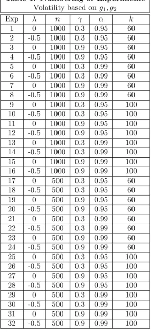
from other previous approaches, to our knowledge, is the consideration of an additional explanatory variable, D. To generalize the performance of our estimator in various conditions, our Monte Carlo simulation method afforded us the flexibility to examine results in a large number of varied conditions while also generating fairly large samples and producing numerous iterations of each scenario. To accomplish this, we varied the individual parameters of the model across 64 different scenarios, which are enumerated in Appendix A, Table 1.
The design of the Monte Carlo aims to yield relative performance metrics for our estimator and a GARCH(1,1) model in a variety of parameter configurations. We designed 64 experiments for the DGP. Table 1 in Appendix A provides the key for how the experiments are numbered in the results section. We consider the following parameter values:
• Two values for sample size: nS ={500,1000}
• Two values forλ: nλ={0,−0.5}
• Two values forγ: nγ ={0.3,0.9}
• Two values for the confidence level,α: nα={0.95,0.99}
• Two values for the number of exceedances,k: nk ={60,100}
• Two functional forms of g(xt), wherextis a linear combination of the regressors, defined by xt=w1yt−1+w2dt−1, are given by
-From Hafner (1998),g1(xt) is given byg1(xt) = 0.5 +
exp(−4xt)
1 +exp(−4xt)
-From Carroll et al. (2002),g2(xt) is given byg2(xt) = 1−0.9exp(−2x2t)
The weightsw1 and w2 are fixed at 0.4 and 0.3, respectively, throughout the Monte Carlo. This
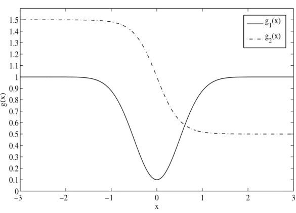
and less weight to the exogenous variable. For our main returns series, the degrees of freedom parameter,v, is held constant at 8. For the exogenous variable, data were generated from a skewed Student-t distribution withv = 3, λ=−0.1, andγ= 0.6, which produces realizations that appear similar to the returns on the S&P 500 from January 3, 1950 to September 30, 2011 by inspection. For each of the 64 experiments, total trials were fixed at 500. Figure 1A in Appendix A illustrates the shapes of theg1(xt) andg2(xt) volatility functions.
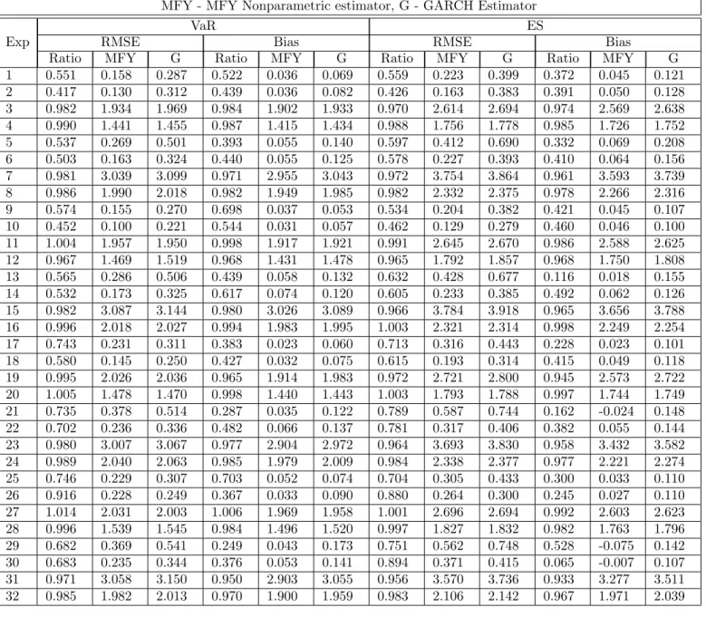
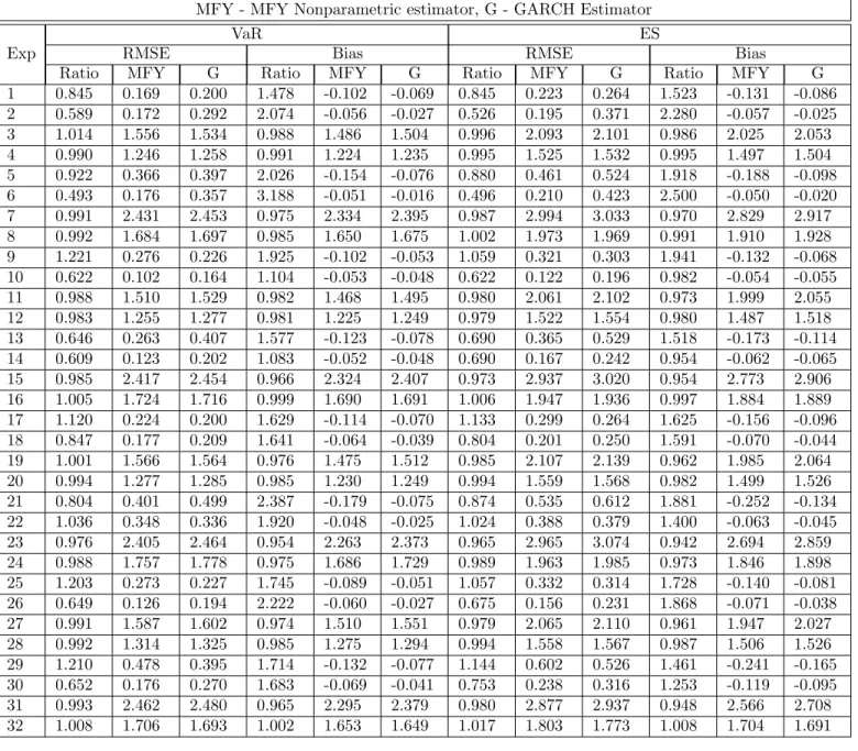
In addition to the estimator considered above, we also performed the same Monte Carlo sim-ulation routine for the MFY estimator. We did this to both attempt to recreate the results of Martins-Filho and Yao (2006) and to provide a basis of comparison for the multivariate estimator presented in this paper. Primarily, we are interested in the impact of adding a second regressor to the estimation procedure as it pertains to the performance metrics of root mean squared error (RMSE) and bias relative to the Gaussian GARCH estimator. We hope to gauge the impact of the curse of dimensionality, which can cripple the local linear estimator in small samples. The optimal rate of convergence of the local regression procedure decreases exponentially with the addition of each dimension (regressor) (Stone (1980)). Therefore, since the sample sizes we consider do not increase for the bivariate case, we expect to see a significant negative change in the performance of our estimator against the GARCH compared with the univariate MFY model, particularly in the case wheren= 500.
5
Results
We considered two first stage estimators for VaR and ES: our nonparametric method and the ARMAX/Gaussian GARCH(1,1) model. For both methods, we only consider the L-moments pro-cedure for the second stage. The considered estimators are based on stochastic models that are intentionally misspecified relative to our DGPs. The nonparametric model is assumed to depend
only onYt−1 and Dt−1 (Markov property of order 1 with an exogenous variable). The GARCH
model is misspecified because it assumes Gaussian innovations and because both g functions we consider are nonlinear functions ofYt−1 andDt−1. In the local linear regression procedure for the
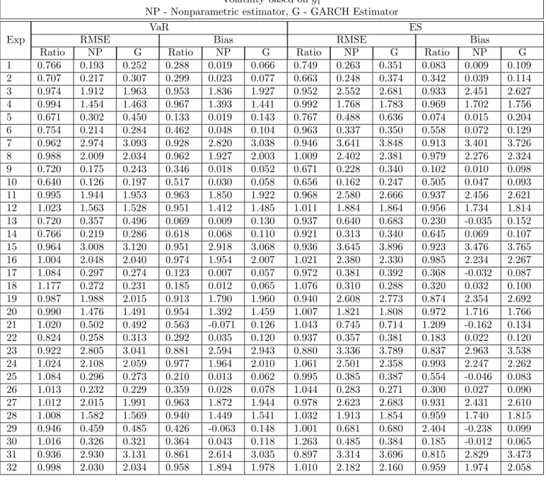
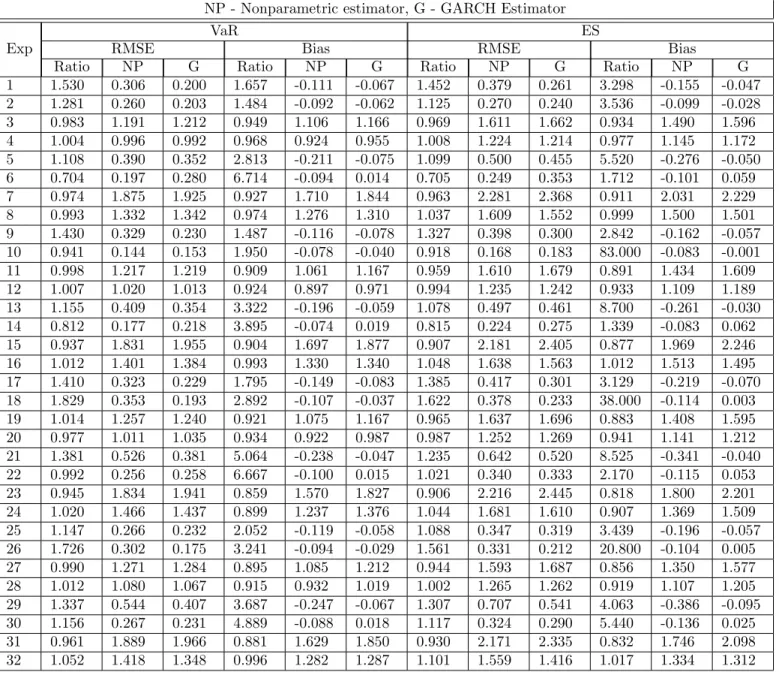
first stage estimators, we use a Gaussian kernel with Ruppert’s theoretical optimal bandwidth. A summary of the Monte Carlo simulation results for our estimator can be found in Appendix 1, Tables 2A and 2B. In Tables 3A and 3B, we present the results obtained from the MFY estimator. The motivation behind including the MFY estimator in the Monte Carlo is twofold: recreating the results of Martins-Filho and Yao (2006) and examining the effect of adding a regressor on the relative performance of the nonparametric estimator versus the GARCH method.
5.1
General Relative Performance
In general, the results for the MFY estimator are consistent with those of our multivariate estimator. One notable exception occurs, however, when we examine the case where n = 500. For both volatility structures, the MFY estimator outperforms GARCH in a similar number of experiments whethern is 1000 or 500. Our bivariate estimator, however, outperforms GARCH in significantly fewer experiments when n = 500. This result indicates that the curse of dimensionality exerts a significant effect on our estimator in small samples sizes. The improvement in performance between
n= 500 andn= 1000 indicates that sufficient convergence of our estimator occurs for ann such that 500< n <1000.
In almost all cases wheren= 1000 and volatility is modeled byg1, the nonparametric estimator
for both VaR and ES outperforms GARCH on the basis of both MSE and bias. Outperformance is much less frequent in cases wheren= 500. We notice for bias in particular that the nonparametric estimator outperforms GARCH in all but two cases. Given that our nonparametric estimator is inherently biased, this is an interesting result because it indicates that the nonlinearities present
in the volatility functiong1 significantly hinder the performance of the GARCH estimator, which
is asymptotically unbiased (Andrews (2009)). For the case where volatility is modeled by g2,
outperformance is witnessed far less frequently for both MSE and bias. An interesting pattern emerges in bias, however in that almost every experiment withγ= 0.9, the nonparametric estimator outperforms relative to GARCH. We do also see more frequent outperformance of the nonparametric estimator in these cases for RMSE, though the pattern isn’t quite as stark as it is for bias. This result is unique tog2 and also appears in our results for the MFY estimator. Our results indicate
that though the nonlinearities of volatility are very important to the performance of our estimator, theγ coefficient also has a significant effect when the volatility is modeled byg2. Additionally, we
note that the nonparametric estimator is consistently less biased than the GARCH estimator for
γ= 0.9, while it always underperforms forγ= 0.3.
Since both estimators are, by construction, misspecified to the actual distribution underlying the data, we expect performance to be related to the shape of the distribution. The results for both
g1andg2support this, as our nonparametric estimator outperforms more frequently in experiments
whereλ=−0.5. Since our GARCH method is defined with normal innovations, it should perform poorly in estimating a skewed distribution, particularly one with heavy skewness such as the case whereλ=−0.5. Our results support this hypothesis.
In both volatility structures, the nonparametric estimator outperformed more frequently for
α= 0.99 than for α= 0.95 when estimating VaR. The opposite is true when estimating ES. This is because, by definition, ES is further out on the tail of the distribution than VaR, which makes ES more difficult to estimate. There is more variance in estimating ES than there is in estimating VaR. GARCH is less able to model VaR further out in the tails as well, which is why we see the nonparametric estimator outperform more frequently whenα= 0.99. Such an effect is muted for
ES. In fact, the nonparametric estimator outperforms GARCH in estimating ES in roughly half the experiments considered. We again attribute this to the curse of dimensionality since the results for the MFY estimator more consistently outperform GARCH for ES. Additionally, RMSE is generally much larger when estimating ES than when estimating VaR.
The number of observations used in the second stage, k, has no significant consistent impact on either the MSE or the bias of any of the estimators considered, ceteris paribus. This results supports the results of Martins-Filho and Yao (2006) and McNeil and Frey (2000).
5.2
Ceteris Paribus Relationships
The results of our Monte Carlo simulation allow us to make severalceteris paribusstatements about the effect of our inputs on the performance of the bivariate nonparametric estimator.
• Sample sizen: In general, asnincreases, RMSE decreases for both volatility models and for both VaR and ES. For three of the four experiment pairings where λ = 0.9 and α= 0.99, the relationship is reversed. The results for bias are mixed; there is no consistent discernible correlation between changing sample size and bias.
• Quantileα: Increasing the quantile from 0.95 to 0.99 increases both RMSE and bias in most experiments for both volatility models and for both VaR and ES. As Martins-Filho and Yao (2006) found, this result indicates that estimation of VaR and ES is more difficult for higher quantiles. For g2, the relationship for RMSE is reversed for three out of four experiment
pairings4 whereγ = 0.3 andλ=−0.5 for both VaR and ES. Such a reversal is not seen for bias.
• Lagged volatility weightγ: As expected, the RMSE for both VaR and ES in both volatility
4When referring to “experiment pairings,” we mean groups of two experiments whose only difference is the
structures increases as γ goes from 0.3 to 0.9. This is true in all experiments. The same relationship holds for bias in all experiments in both volatility structures and for both VaR and for ES. In all experiment pairs where volatility is modeled byg2 bias goes from negative
to positive asγgoes from 0.3 to 0.9. The nonparametric estimator tends to underpredict VaR and ES when lagged volatility is weighted less and tends to overpredict VaR and ES when lagged volatility is weighted more heavily.
• Skewness parameterλ: The RMSE decreases significantly for all but one experiment asλgoes from 0 to -0.5. This relationship is likely explained by the fact that our DGP, whenλ≤0, is skewed toward the positive quadrant. Therefore, in the second stage of our estimation procedure, when we select data larger than thekthorder statistic, we, by default, select data more representative of tail behavior whenλdecreases. Contradictory to the results found by Martins-Filho and Yao (2006), there is a clear pattern that emerges in bias asλdecreases. In all but two experiment pairings forg2, bias decreases along withλ. Forg1, a regular pattern
emerges where for all experiments withγ= 0.9, decreasingλdecreases bias for both VaR and ES, while for all experiments where γ = 0.3, decreasing λ increases bias for both VaR and ES.
• Number of exceedances k: The impact of increasing k from 60 to 100 is unclear. For g1,
increasingk tends to increase RMSE and bias in a majority of cases, but the relationship is far from definitive. Forg2, the results are mixed enough that no obvious relationship emerges.
These results generally indicate that our bivariate nonparametric estimator outperforms GARCH in larger samples. By including a largern, we notice significantly better performance in both volatil-ity constructs, though the effect is more pronounced forg1(x).
6
Conclusion
In this paper we have proposed a modification of the method for estimating VaR and ES proposed by Martins-Filho and Yao (2006). Due to the popularity and widespread use of VaR and ES in the empirical and theoretical literature as well as in professional applications, a better understanding of market risk estimation is paramount to sound financial management. Our procedure extends the methodology used by Martins-Filho and Yao (2006) by generalizing it to the multivariate case, specifically by adding one exogenous variable. We used local linear regression techniques in stage one of our estimation procedure and L-moments and EVT in stage two to estimate the one-period forecasted VaR and ES. The Gaussian GARCH model is employed as an alternative first stage es-timator for ˆmand ˆσ2for comparative purposes. Our Monte Carlo simulation is based on a skewed
Student-t distributed DGP that incorporates many of the empirically observed characteristics of financial returns series. The Monte Carlo simulation indicates that our estimation method outper-forms the GARCH methodology, but does so much more consistently whenn= 1000. We contend that what underperformance is present is due primarily to the curse of dimensionality. To our knowledge, this is the first evidence of the finite sample performance of VaR and ES estimators in multivariate conditional densities, particularly with consideration of exogenous variables. The results from our simulation indicate that nonlinearities in volatility dynamics exert a significant ef-fect on estimates of risk. Concurrent with the findings of Martins-Filho and Yao (2006), this result indicates that accounting for the nonlinearities in volatility is more important than more compre-hensive modeling of temporal dependence. More investigation is necessary, however, to determine the performance of our estimator in a greater variety of parameter configurations.
Areas for Further Research: There remain several avenues for further investigation into
limitations on computing power and time. Future researchers may find examining additional cases in the simulation, particularly those which consider larger sample sizes, to yield interesting results. Additionally, consideration of a larger variety of GARCH variants would reveal a more complete picture of the relative performance of our estimators. Researchers more concerned with the local regression procedure may also be interested in exploring the performance of a local polynomial estimators, assuming continuity assumptions are relaxed. With greater computing power and more time, it may also be interesting to examine the effects of adding more lags and more exogenous variables to the DGP. Researchers examining this question, however, would need to consider ex-tremely large sample sizes. That said, a comprehensive backtesting evaluation of the estimator on actual historical financial time series would provide a glimpse into the real-world performance of our estimator compared to the methods currently employed by practitioners. One useful modifi-cation of this model would be to redefine the estimator in terms of an additive model. Doing so would mitigate the impact of the curse of dimensionality and allow the estimator to converge at nearly the rate of the GARCH model (Andersen et al. (2009)). In fact, the best possible rate of convergence for estimates ofσ2t is equal to that of the univariate nonparametric regression (Stone
(1985)). The additive version, is, however, more restrictive on the functional form of the estimator. Finally, like the method set forth by Martins-Filho and Yao (2006), the asymptotic characteristics of these estimators are also yet unknown and could prove interesting to the theoretical researcher.
A
Appendix A - Tables and Graphs
Figure 1: Conditional Volatility based on g1(x)and g2(x)where x=X(Yt−1, dt−1)
−3
0
−2
−1
0
1
2
3
0.1
0.2
0.3
0.4
0.5
0.6
0.7
0.8
0.9
1
1.1
1.2
1.3
1.4
1.5
x
g(x)g
1(x)
g
2(x)
Table 1: Numbering of Experiments Volatility based ong1, g2 Exp λ n γ α k 1 0 1000 0.3 0.95 60 2 -0.5 1000 0.3 0.95 60 3 0 1000 0.9 0.95 60 4 -0.5 1000 0.9 0.95 60 5 0 1000 0.3 0.99 60 6 -0.5 1000 0.3 0.99 60 7 0 1000 0.9 0.99 60 8 -0.5 1000 0.9 0.99 60 9 0 1000 0.3 0.95 100 10 -0.5 1000 0.3 0.95 100 11 0 1000 0.9 0.95 100 12 -0.5 1000 0.9 0.95 100 13 0 1000 0.3 0.99 100 14 -0.5 1000 0.3 0.99 100 15 0 1000 0.9 0.99 100 16 -0.5 1000 0.9 0.99 100 17 0 500 0.3 0.95 60 18 -0.5 500 0.3 0.95 60 19 0 500 0.9 0.95 60 20 -0.5 500 0.9 0.95 60 21 0 500 0.3 0.99 60 22 -0.5 500 0.3 0.99 60 23 0 500 0.9 0.99 60 24 -0.5 500 0.9 0.99 60 25 0 500 0.3 0.95 100 26 -0.5 500 0.3 0.95 100 27 0 500 0.9 0.95 100 28 -0.5 500 0.9 0.95 100 29 0 500 0.3 0.99 100 30 -0.5 500 0.3 0.99 100 31 0 500 0.9 0.99 100 32 -0.5 500 0.9 0.99 100
Table 2A: Root MSE and Bias
Volatility based ong1
NP - Nonparametric estimator, G - GARCH Estimator Exp
VaR ES
RMSE Bias RMSE Bias
Ratio NP G Ratio NP G Ratio NP G Ratio NP G
1 0.766 0.193 0.252 0.288 0.019 0.066 0.749 0.263 0.351 0.083 0.009 0.109 2 0.707 0.217 0.307 0.299 0.023 0.077 0.663 0.248 0.374 0.342 0.039 0.114 3 0.974 1.912 1.963 0.953 1.836 1.927 0.952 2.552 2.681 0.933 2.451 2.627 4 0.994 1.454 1.463 0.967 1.393 1.441 0.992 1.768 1.783 0.969 1.702 1.756 5 0.671 0.302 0.450 0.133 0.019 0.143 0.767 0.488 0.636 0.074 0.015 0.204 6 0.754 0.214 0.284 0.462 0.048 0.104 0.963 0.337 0.350 0.558 0.072 0.129 7 0.962 2.974 3.093 0.928 2.820 3.038 0.946 3.641 3.848 0.913 3.401 3.726 8 0.988 2.009 2.034 0.962 1.927 2.003 1.009 2.402 2.381 0.979 2.276 2.324 9 0.720 0.175 0.243 0.346 0.018 0.052 0.671 0.228 0.340 0.102 0.010 0.098 10 0.640 0.126 0.197 0.517 0.030 0.058 0.656 0.162 0.247 0.505 0.047 0.093 11 0.995 1.944 1.953 0.963 1.850 1.922 0.968 2.580 2.666 0.937 2.456 2.621 12 1.023 1.563 1.528 0.951 1.412 1.485 1.011 1.884 1.864 0.956 1.734 1.814 13 0.720 0.357 0.496 0.069 0.009 0.130 0.937 0.640 0.683 0.230 -0.035 0.152 14 0.766 0.219 0.286 0.618 0.068 0.110 0.921 0.313 0.340 0.645 0.069 0.107 15 0.964 3.008 3.120 0.951 2.918 3.068 0.936 3.645 3.896 0.923 3.476 3.765 16 1.004 2.048 2.040 0.974 1.954 2.007 1.021 2.380 2.330 0.985 2.234 2.267 17 1.084 0.297 0.274 0.123 0.007 0.057 0.972 0.381 0.392 0.368 -0.032 0.087 18 1.177 0.272 0.231 0.185 0.012 0.065 1.076 0.310 0.288 0.320 0.032 0.100 19 0.987 1.988 2.015 0.913 1.790 1.960 0.940 2.608 2.773 0.874 2.354 2.692 20 0.990 1.476 1.491 0.954 1.392 1.459 1.007 1.821 1.808 0.972 1.716 1.766 21 1.020 0.502 0.492 0.563 -0.071 0.126 1.043 0.745 0.714 1.209 -0.162 0.134 22 0.824 0.258 0.313 0.292 0.035 0.120 0.937 0.357 0.381 0.183 0.022 0.120 23 0.922 2.805 3.041 0.881 2.594 2.943 0.880 3.336 3.789 0.837 2.963 3.538 24 1.024 2.108 2.059 0.977 1.964 2.010 1.061 2.501 2.358 0.993 2.247 2.262 25 1.084 0.296 0.273 0.210 0.013 0.062 0.995 0.385 0.387 0.554 -0.046 0.083 26 1.013 0.232 0.229 0.359 0.028 0.078 1.044 0.283 0.271 0.300 0.027 0.090 27 1.012 2.015 1.991 0.963 1.872 1.944 0.978 2.623 2.683 0.931 2.431 2.610 28 1.008 1.582 1.569 0.940 1.449 1.541 1.032 1.913 1.854 0.959 1.740 1.815 29 0.946 0.459 0.485 0.426 -0.063 0.148 1.001 0.681 0.680 2.404 -0.238 0.099 30 1.016 0.326 0.321 0.364 0.043 0.118 1.263 0.485 0.384 0.185 -0.012 0.065 31 0.936 2.930 3.131 0.861 2.614 3.035 0.897 3.314 3.696 0.815 2.829 3.473 32 0.998 2.030 2.034 0.958 1.894 1.978 1.010 2.182 2.160 0.959 1.974 2.058